Sage Journals: Discover world-class research

Abstract

A retailer places orders periodically for items that are shipped by a wholesaler. Items that are not sold perish randomly and independently of one another, with the perish probability depending on the age class. We consider a first‐in‐first‐out policy for depleting items. We model this problem as a Markov decision process with stochastic demand, unit holding, outdating and ordering costs, plus unit penalty costs for lost sales. We prove convexity for the penultimate period and show convexity may not hold any earlier. A dynamic program can be solved optimally for small instances. We introduce both a one‐stage‐lookahead heuristic and a heuristic which is a combination of two existing standard approaches, the newsvendor and periodic review models. For simulated data, we compare these heuristics to the optimal solution for small problem instances and to further lookahead policies for larger problem instances. We show that the two new heuristics achieve results close to optimal. Our numerical study, which includes real data from a large European retail chain, highlights that products perishing independently from each other strongly affect model behavior compared to existing approaches from the literature.

Keywords

age‐dependent lifetime inventory management perishables random lifetime

INTRODUCTION

Managing inventories for perishable products poses an important challenge to retailers for several reasons. Items perishing is costly due to the loss of revenue and potential disposal costs. Since the lifetime of fresh products is often random, the retailer does not know exactly how long a product will remain salable before it spoils which makes it difficult to determine future inventory. Furthermore, customers expect high availability of fresh products such as fruit and vegetables, with consequences if these expectations are not met. Namely, fresh products attract customers, who then buy other products that are on their shopping list at the same store. Therefore, if fresh products stock out, profitability of the whole store suffers, since customers may decide to buy all their products elsewhere and may not return in the future due to the inconvenience caused. Consequently, managing perishable products efficiently is crucial to the profitability of groceries in the retail industry. By taking the characteristics of customer demand and the perishability process into account, retailers can make better inventory decisions which balance satisfying customer needs and minimizing spoilage.

In this paper, we focus on food products. However, our model also applies to other settings such as the healthcare industry, within, for example, blood supply management. Red blood cells can be transfused up to 42 days after donation (Sarhangian et al., 2018), and blood platelets have a lifetime of only 5 days (Chao et al., 2018; Chen et al., 2019). Perishability is of special importance to blood platelets, since they are expensive to purchase, store and dispose, and lives may be put at risk if their management is not planned carefully (Duan & Liao, 2013; Haijema et al., 2007).

We consider store managers' ordering decisions for perishable products in the setting of a large European retail chain where customers pick older items first, that is, according to a first‐in‐first‐out (FIFO) policy. The FIFO policy is preferred by retailers because it helps to reduce spoilage. Hence, newer items are placed in boxes under the older items or kept in the backroom storage and cold room (Reiner et al., 2013). FIFO is also commonly used in the literature (e.g., Chao et al., 2015; Karaesmen et al., 2011; Ketzenberg et al., 2015; Nahmias, 2011).

When placing an order, it is important for the retailer to forecast both future demand and the amount of products that will perish. Customer demand is stochastic and varies from day to day. The perishing process is characterized by two measures. One is the maximum shelf life, which is the maximum number of days a product can be sold. The other is the perish probability, which determines the probability with which a product has to be discarded at the end of a day. A product perishing affects the retailer both by incurring an outdating cost and by depleting the inventory available for the next day. The closer an item is to its maximum shelf life, the more likely it is to perish.

We model the retailer's problem as a periodic review inventory control model with lost sales. Customer demand has an arbitrary distribution that we do not require to be stationary. In each period, any item perishes independently of the others with a known, age‐dependent perish probability. Therefore, items may perish out of sequence, that is, in a different order than they arrived. Any perished item incurs an outdating cost, but there is also a per‐item penalty cost for unfulfilled demand. We formulate our model as a Markov decision process (MDP).

Our setting is similar to the one analyzed by Ketzenberg et al. (2015), but with two important extensions. The first is nonstationary demand, which is frequently observed in retailing, where demand tends to be higher at weekends. The second is all items perishing independently; Ketzenberg et al. (2015) assume dependent perishing where items of the same age class all perish at the same time. Our independence assumption increases the number of possible state transitions but is more realistic for the retail setting we consider; for example, one bad pack of strawberries does usually not spoil the whole batch. As we will show in our numerical study, independent perishing strongly affects model behavior so dependent perishing is not a good substitute.

To demonstrate the practical use of our model, we collected hourly data from a large European retail chain over a time horizon of 2 years for 66 stores. We analyze sales data and selling prices for five perishable products (fruit and vegetables) with a range of maximum shelf lives and age‐dependent perish probabilities. The store managers currently use their own judgment to make order decisions, and the retail chain is considering using commercial software solutions in the future that would contain standard methods such as the periodic review or newsvendor model. In this paper, we compare such standard methods to the optimal solution and the heuristics we develop.

The paper proceeds as follows. In Section 2, we review the literature on periodic review models with perishable products. The following sections make several contributions to this literature. In Section 3, we propose a new model for a real‐life problem—the periodic review model with independent age‐dependent lifetimes and lost sales. We also develop a simplifying cost transformation, a lower bound on the optimal cost and show that convexity holds in the penultimate period but may fail earlier.

For instances with a small state space, we obtain optimal solutions via dynamic programming. Each state can have a large number of follow‐up states when inventories are large and maximum shelf lives long, so many realistic problem instances are computationally infeasible to solve optimally. Therefore, in Section 4, we introduce two heuristics tractable for larger problem instances. In Section 5, we analyze the performance of these two heuristics for both simulated and the aforementioned real data from the retail chain. We compare their performance both to each other and to simple order policies which either assume that items always perish (newsvendor model) or never perish (periodic review model). We show that there is a clear benefit from using these heuristics instead of simple policies, which are often applied in practice. In addition, our numerical results indicate that, in any considered problem case, at least one of our two heuristics is always close to optimality.

LITERATURE REVIEW

We review the literature of periodic review models for perishable products and stochastic demand. We distinguish between models that assume a fixed lifetime, and those that consider random lifetimes, which is also related to the literature on random yield.

Fixed lifetime

Research on fixed lifetime inventory systems originated with Van Zyl (1964), where the periodic review setting with backorders, stochastic demand, a FIFO inventory depletion policy, and a fixed lifetime of two periods is analyzed. Upper and lower bounds on the cost function are derived, and a nonstationary optimal ordering policy is shown to exist. Nahmias and Pierskalla (1973) add a per‐item perish cost to this model, and Nahmias (1975) further extends to a lifetime of n periods. A myopic policy based on an approximated outdating distribution function is developed in Nahmias (1976).

The model of Nahmias (1975) has also been studied with lost sales instead of backorders. Nandakumar and Morton (1993) utilize expected outdate bounds similarly to Nahmias (1976) to derive a heuristic. Chao et al. (2015) investigate nonstationary demand which can be correlated to account for seasonality. They introduce two policies that balance cost components and derive worst‐case performance bounds. They show that their results hold both for the backlogging and lost‐sales settings. Williams and Patuwo (1999) assume a lifetime of two periods but allow positive lead times. They derive optimal order quantities for lead times of up to four periods. Minner and Transchel (2010) analyze a model with positive lead times under service‐level constraints. Using their analysis of the inventory distribution, they compare a dynamic order size policy with constant order and base‐stock policies. Haijema and Minner (2016) provide further insight into fixed lifetime models by comparing the performances of constant order policies, base stock policies, and hybrid policies that also take age‐dependent inventories into account. Recently, Haijema and Minner (2019) consider a model with batch sizes and a mixture of demand via FIFO and last‐in‐first‐out (LIFO) depletion policies. They propose new solution policies based on a division of stock into new and old products which reduces the complexity.

Random lifetime

The majority of the random lifetime literature concerns continuous review models. Indeed, Ketzenberg et al. (2015) point out that by the time of publication of their paper, only they and Nahmias (1977) consider a periodic review model for perishable products with random lifetime and stochastic demand. Nahmias (1977) extends the model by Nahmias (1975) to a stochastic lifetime while assuming that successive goods outdate in the same order that they arrive and that all goods of the same age perish or survive jointly. Using a similar approach as Nahmias (1976), an adjusted myopic policy is derived.

Ketzenberg et al. (2015) address the random lifetime setting of Nahmias (1977) for lost sales. While they drop the assumption that products perish in the order in that they arrive, they do assume that all items in the same age group perish together. They evaluate the value of time and temperature history to determine the quality of goods. Assuming a lead time of one period, an infinite time horizon, and a stationary demand distribution, they develop heuristics that trade off simplicity and performance.

Kouki and Jouini (2015) study the effect of random lifetimes on the performance of inventory systems. They develop an analytical solution for exponential and deterministic lifetime distributions and conduct a simulation study for the more general case of Erlang distributions. For a comprehensive review of the literature on all types of inventory systems, see Bakker et al. (2012), Goyal and Giri (2001), Janssen et al. (2016), Karaesmen et al. (2011), and Nahmias (1982).

The periodic‐review inventory problem that we consider with stochastic demand, lost sales, and age‐dependent perishability where each item perishes independently has not been analyzed in the literature, despite this being a very common problem in retailing. Standard models from the literature solve extreme cases of our problem where either all or no items perish each day. We assess both these standard models and the age‐group‐dependent perishing model of Ketzenberg et al. (2015) in our independent‐perishing setting.

Random yield

Related to modeling random lifetimes is the literature on random yield, as only a portion of the products makes it to the next period due to the probability of an item perishing. For example, Voelkel et al. (2020) suggest an MDP that considers random yield during transport where either all or none of the items can spoil in each lead time period. Sonntag and Kiesmüller (2017) also regard stochastic demand and random yield in a multistage system. They introduce quality control systems to monitor the effect of random yield and achieve significant safety stock reductions. Kiesmüller and Inderfurth (2018) propose a periodic‐review model with order inflation to solve the multiperiod inventory control problem with stochastic demand, fixed setup costs, and random production yield. They show that simple heuristics can perform very well for this complex problem if the parameters are adjusted to demand and yield risks appropriately. For a more extensive overview of the literature on random yield models, see Yano and Lee (1995) and, more recently, Kiesmüller and Inderfurth (2018).

Even though our setting is similar to random yield problems, common policies such as order inflation cannot be applied: the inflation factor would ignore the fact that inventory in the first period is not subject to random yield as no perishing has occurred yet. Furthermore, the inflation factor does not take the age structure into account, which is important in our setting with age‐dependent perish probabilities.

MODEL

In this section, we formulate the mathematical basis for analyzing the stochastic periodic review model of a single stock‐keeping unit with a random and age‐dependent lifetime. We choose a finite horizon over a planning horizon of T periods, indexed by
$t = 1, …, T$
. In‐stock units have a maximum lifetime of m periods. We assume that items perish independently of one another, each according to a Bernoulli distribution. The complete notation is summarized in Supporting Information Section EC.1.

Sequence of events

First, the retailer observes the state of the inventory:
$x_{t} \equiv (x_{t, 1}, …, x_{t, m})$
denotes the discrete numbers of units in stock at the start of period t, where
$x_{t, i}$
denotes those of age class i, in other words, those ordered in period
$t - i$
. The total on‐hand inventory is denoted
$x_{t} \equiv \sum_{i = 1}^{m} x_{t, i}$
. Second, the retailer places an order
$q_{t}$
. Third, a random demand
$D_{t}$
occurs with the probability function
$f_{D_{t}} (\cdot)$
. According to the FIFO inventory depletion policy, units with the highest age class are purchased first. If
$D_{t}$
exceeds
$x_{t}$
, then excess demand is lost and a per‐unit shortage penalty cost incurred. Otherwise, each unsold item incurs an inventory holding cost. Fourth, any unsold units perish independently of one another and the retailer disposes of perished units at per‐unit outdating costs. Fifth, the ordered
$q_{t}$
units arrive. This corresponds to an effective lead time of one period, which is common in retailing.

Inventory transition

We write
$Y_{t} \equiv (Y_{t, 1}, …, Y_{t, m})$
for the inventory vector between steps 3 and 4 in the sequence of events above, in other words, after demand has occurred but before perishing and before orders have arrived. Where
${[x]}^{+} \equiv \max (0, x)$
for any variable x,
$Y_{t, i} = {[x_{t, i} - {[D_{t} - \sum_{j = i + 1}^{m} x_{t, j}]}^{+}]}^{+}$
follows directly from the FIFO depletion policy. Throughout we use capital letters for random variables and small letters for their realizations. Therefore, we write
$y_{t, i} (d_{t}) = {[x_{t, i} - {[d_{t} - \sum_{j = i + 1}^{m} x_{t, j}]}^{+}]}^{+}$
for the realization of
$Y_{t, i}$
where demand
$d_{t}$
occurs. Analogously to known inventory x _t, we denote the vector of random inventories of different age classes at the start of period t as
$X_{t} \equiv (X_{t, 1}, …, X_{t, m})$
and their sum as
$X_{t}$
.

Newly ordered items have no yield loss, so
$x_{t + 1, 1} = q_{t}$
. Units of other age classes transfer according to a binomial distribution, that is
$X_{t + 1, i + 1} = \sum_{j = 1}^{Y_{t, i}} Φ_{i, j}$
for
$1 \leq i \leq m - 1$
, where
$Φ_{i, j}$
are independently and identically distributed Bernoulli‐distributed random variables with parameter
$(1 - ψ_{i})$
. The parameter
$ψ_{i}$
denotes the perish probability for an item of age class i. Because the maximum lifetime is m,
$ψ_{m} = 1$
.

For
$m = 3$
, Table 1 shows a sample trajectory that illustrates the dynamics of the process. We start with an inventory x ₁ that consists of four, three, and five items of age classes 1, 2, and 3, respectively. In
$t = 1$
, we order
$q_{1} = 7$
items and a demand of
$d_{1} = 4$
occurs. Following the FIFO depletion policy, four items of age class 3 are sold. Next, items in y ₁ perish independently with probability depending on the age class. In the example, two of the four age 1 items perish and none of the three age 2 items perish. Since the maximum lifetime is 3, the one unsold age 3 item perishes with certainty. The remaining items of ages 1 and 2 then form age classes 2 and 3 of x ₂, respectively, with the
$q_{1} = 7$
items forming age class 1. In
$t = 2$
, we order
$q_{2} = 9$
items and observe a demand of
$d_{2} = 6$
. The demand depletes age classes 2 and 3 completely and uses one item of age class 1. Afterwards, one age 1 item perishes, and x ₃ is formed both by the remaining inventories shifting by one age class and the
$q_{2} = 9$
items arriving. In
$t = 3$
, we order
$q_{3} = 4$
items and the demand of
$d_{3} = 15$
items consumes the entire inventory, with one unit of demand left unsatisfied.

TABLE 1
Example state transition

t x _t $q_{t}$
$d_{t}$
y _t Perished units

1 (4,3,5) 7 4 (4,3,1) (2,0,1)

2 (7,2,3) 9 6 (6,0,0) (1,0,0)

3 (9,5,0) 4 15 (0,0,0) (0,0,0)

Total cost

The cost components of our model are variable ordering, holding, penalty, and outdating costs. Ordering costs
$c q_{t}$
are linear in the order size. We mark variables with a hat that will change based on a simplifying cost transformation (Proposition 1) presented later in this section. Holding costs are
$\hat{h} {[x_{t} - D_{t}]}^{+}$
, and shortage penalty costs are
$\hat{p} {[D_{t} - x_{t}]}^{+}$
. The number of outdated units is
$E_{t} \equiv \sum_{i = 1}^{m} B_{t, i} (Y_{t, i}, ψ_{i})$
, where
$B_{t, i} (n, ψ)$
denotes a binomially distributed random variable with parameters n and ψ. Outdating costs are
$\hat{θ} E_{t}$
. We assume that
$c, \hat{p}, \hat{h}$
, and
$\hat{θ}$
are nonnegative.

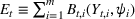
The one‐period cost function, given order
$q_{t}$
and inventory x _t, is
${\hat{G}}_{t} (x_{t}, q_{t}) \equiv c q_{t} + \hat{h} {[x_{t} - D_{t}]}^{+} + \hat{p} {[D_{t} - x_{t}]}^{+} + \hat{θ} E_{t},$
1and the costs over the whole planning horizon T are
$\hat{G} (q) \equiv \sum_{t = 1}^{T} γ^{t - 1} {\hat{G}}_{t} (X_{t}, q_{t}) - γ^{T - 1} c x_{T + 1},$
2where γ is a discount factor and q is the vector of orders from
$t = 1$
to T.

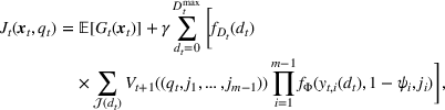
Note that (2) assumes that excess inventory can be salvaged at unit salvage value c at the end of the time horizon. The salvage value of older products would usually be less than 100% of the order cost c; however, the salvage value only affects the final period T, which is in the distant future, so the effect on the overall model is minimal. We conducted a sensitivity analysis to demonstrate this. For the 135 problem instances in the numerical study described in Section 5.1, if the 100% salvage value for all items is replaced by 50%, then the optimal costs rise on average only by 0.03%. If the 100% is replaced by 0%, the same rise is 0.05%. The benefit of assuming a 100% salvage value is that it allows the cost structure to be simplified, as will be seen later in this section in Proposition 1.

Our objective is to find the optimal cost
$\min_{q} \hat{G} (q)$
and the associated optimal policy. To do this, we formulate our model as an MDP with the Bellman equation
${\hat{V}}_{t} (x_{t}) = \min_{q_{t}} {\hat{J}}_{t} (x_{t}, q_{t})$
3for
$1 \leq t \leq T$
with
${\hat{J}}_{t} (x_{t}, q_{t}) = E [{\hat{G}}_{t} (x_{t}, q_{t})] + γ {\hat{V}}_{t + 1} (X_{t + 1})$
and terminal function
${\hat{V}}_{T + 1} (x_{T + 1}) = - γ^{- 1} c x_{T + 1}$
. Let
$J (d_{t}) \equiv {(j_{1}, …, j_{m - 1}) : 0 \leq j_{i} \leq y_{t, i} (d_{t}), 1 \leq i \leq m - 1}$
be the set of all possible combinations of inventories after perishing, given demand realization
$d_{t}$
. Considering the randomness of both the outdating process and the customer demand, we obtain
$\begin{matrix} {\hat{J}}_{t} (x_{t}, q_{t}) & = & E [{\hat{G}}_{t} (x_{t}, q_{t})] + γ \sum_{d_{t} = 0}^{D_{t}^{\max}} [f_{D_{t}} (d_{t}) \\ \times \sum_{J (d_{t})} {\hat{V}}_{t + 1} ((q_{t}, j_{1}, …, j_{m - 1})) \prod_{i = 1}^{m - 1} f_{Φ} (y_{t, i} (d_{t}), 1 - ψ_{i}, j_{i})] \end{matrix}$
4for
$1 \leq t \leq T$
, where
$f_{Φ} (n, ψ, k) \equiv (\binom{n}{k}) ψ^{k} {(1 - ψ)}^{n - k}$
is the probability function of the binomial distribution with parameters n and ψ, and we assume that the demand
$D_{t}$
is bounded above by
$D_{t}^{\max}$
.

Equation (3) allows us to find the optimal solution using dynamic programming. The curse of dimensionality renders this method computationally intractable for large problem instances. For example, with
$m = 3$
,
$D^{\max} = 50$
, and
$T = 200$
, the optimal solution takes around 12 hours to calculate, which is not practically useful. However, we will utilize the MDP formulation to analyze the problem's structure and to subsequently obtain heuristic policies. We will also calculate optimal solutions for small problem instances and will use them as a benchmark for our heuristics.

For any problem instance, we may use the MDP structure to form a lower bound on the optimal cost using the following observation. If there is no maximum lifetime and the perish probabilities for each age are all the same, then the age of an item is insignificant, so the state of the MDP is simply the total inventory
$x_{t}$
. This leads to a drastic reduction of the state space, and an MDP which is quick to solve. While an unrealistic model, if we set
$ψ \equiv \min_{i = 1, …, m} ψ_{i}$
as the perish probability for all ages (in other words, the number of perished items follows a binomial distribution with parameter ψ) we obtain a problem whose optimal cost is an easily calculable lower bound for the problem with maximum lifetime m and perish probabilities
$ψ_{1}, …, ψ_{m}$
. We will investigate the lower bound numerically in Section 5.4.

Next, similarly to Chao et al. (2015), we modify
$\hat{h}$
,
$\hat{p}$
, and
$\hat{θ}$
to absorb part of the per unit order cost c, so the only order cost remaining is paid at the terminal time and is independent of the order policy. This simplifies the structure of the model and the convexity proof of Proposition 2 because the cost incurred in period t is independent of the order
$q_{t}$
.

We formulate this simplification in Proposition 1. The proof of the proposition follows a similar structure to Chao et al. (2015). The proof can be found in Supporting Information Section EC.2. Proposition 1
We define h as
$\hat{h} + (γ^{- 1} - 1) c$
, p as
$\hat{p} - γ^{- 1} c$
and θ as
$\hat{θ} + c$
. Then,
$V_{t} (x_{t}) = \min_{q_{t}} J_{t} (x_{t}, q_{t})$
5for
$1 \leq t \leq T$
with
$\begin{matrix} J_{t} (x_{t}, q_{t}) & = & E [G_{t} (x_{t})] + γ \sum_{d_{t} = 0}^{D_{t}^{\max}} [f_{D_{t}} (d_{t}) \\ \times \sum_{J (d_{t})} V_{t + 1} ((q_{t}, j_{1}, …, j_{m - 1})) \prod_{i = 1}^{m - 1} f_{Φ} (y_{t, i} (d_{t}), 1 - ψ_{i}, j_{i})], \end{matrix}$
6
$G_{t} (x_{t}) = h {[x_{t} - D_{t}]}^{+} + p {[D_{t} - x_{t}]}^{+} + θ E_{t}$
7and with the terminal cost function
$V_{T + 1} (x_{T + 1}) \equiv V_{T + 1} = γ^{- T} \sum_{t = 1}^{T} γ^{t - 2} c E [D_{t}]$
8is an equivalent MDP to the one formulated in (3).

Convexity holds at the penultimate period. The proof of the below can be found in Supporting Information Section EC.3. Proposition 2
For any inventory
$x_{T - 1}$
,
$J_{T - 1} (x_{T - 1}, q_{T - 1})$
is convex in
$q_{T - 1}$
.

Before the penultimate period, convexity of
$J_{t}$
in
$q_{t}$
is not guaranteed. In the following, we show a counterexample where
$J_{T - 2}$
is not convex.

Let
$T = 3$
, the maximum lifetime
$m = 2$
, and the discount factor
$γ = 1$
. Write
$ψ \equiv ψ_{1}$
for the perish probability of age one items. The inventory state at time t is represented by the 2‐tuple
$x_{t} \equiv (x_{t, 1}, x_{t, 2})$
. Suppose
$D_{t} = 3$
for
$t = 1, 2, 3$
, which has the following implications:
The retailer never optimally orders more than three items, since any excess on three items will not sell at age one and hence incur an unnecessary holding cost. Therefore, we may restrict the retailer to orders of at most three, which, assuming the starting age i stock level
$x_{1, i} \leq 3$
for
$i = 1, 2$
, means
$x_{t, i} \in {0, 1, 2, 3}$
for
$t = 1, 2, 3$
, restricting the state space.

Under this restriction of the state space, at any time period, all the age two items will sell (so none perish). Therefore, any unsold items must be age one (which perish with probability ψ), so the state can be delineated by the total inventory
$x_{t} \equiv x_{t, 1} + x_{t, 2}$
, leading to a state space of
${0, …, 6}$
.

In Supporting Information Section EC.4, we show that, when
$ψ < 0.147$
and
$2 p ψ = (1 - ψ) (h + ψ θ)$
, we have
$J_{1} (6, 3) - 2 J_{1} (6, 2) + J_{1} (6, 1) < 0;$
9in other words,
$J_{1} (6, q_{1}) = J_{T - 2} (6, q_{1})$
is not convex in q ₁.

HEURISTIC POLICIES

In this section, we develop and analyze heuristic policies. First, we discuss two policies which are often used in practice but are designed for the simple cases where either all or no product perishes. In Section 4.1, we introduce a Newsvendor policy optimal for the case where all product perishes, and in Section 4.2 a periodic review policy which assumes no product perishes. Next, in Section 4.3, we develop our own heuristic, which is a novel combination of the previous two. In Section 4.4, we analyze the ordering behavior of all three heuristics immediately evident from their formulae. Finally, in Section 4.5, we develop policies looking several periods ahead, with a particular focus on the one‐stage lookahead policy due to the convexity of our model at time
$T - 1$
.

Newsvendor heuristic

First, suppose all items perish after one period; this is a newsvendor model. Since the inventory is emptied at the end of each period, the optimal order at period t (
$q_{t}^{NV}$
) is the optimal base‐stock level at the start of time
$t + 1$
, which is known to be
$q_{t}^{NV} \equiv F_{D_{t + 1}}^{- 1} (\frac{p}{p + h + θ}),$
10where
$F_{D}^{- 1}$
represents the generalized inverse cumulative distribution function of the random variable D (Axsäter, 2015). We call (10) the newsvendor heuristic (NV). Note the quantile in (10) balances the underage cost, p, and the overage cost,
$h + θ$
.

Periodic review heuristic

Now suppose items do not perish at all; this is a standard periodic review model. Once an item is ordered, it remains in the inventory until it is sold, so its age is immaterial. Therefore, the state is simply the total inventory, denoted
$x_{t}$
at time t. In the following, we present a simple heuristic arising from this model.

If items never perish, the overage cost per unit time is h. Since the underage cost is still p, by (10), the optimal base‐stock level at the start of time
$t + 1$
is
$F_{D_{t + 1}}^{- 1} (\frac{p}{p + h})$
. If the retailer knew at time t the on‐hand stock at time
$t + 1$
, namely
$x_{t + 1} = \max (x_{t} - d_{t}, 0)$
, then the optimal order at time t (
$q_{t}^{PRV}$
) would be
$q_{t}^{PRV} \equiv \max (0, F_{D_{t + 1}}^{- 1} (\frac{p}{p + h}) - \max (x_{t} - d_{t}, 0)),$
11in words, order to bring
$x_{t + 1}$
up to
$F_{D_{t + 1}}^{- 1} (\frac{p}{p + h})$
, or order 0 if
$x_{t + 1}$
already exceeds
$F_{D_{t + 1}}^{- 1} (\frac{p}{p + h})$
. Yet, the retailer does not know
$d_{t}$
at time t, so cannot compute
$q_{t}^{PRV*}$
when making the time t order. A sensible heuristic estimates
$x_{t + 1}$
using its expectation over the demand at time t, then rounds to the nearest integer, ordering
$q_{t}^{PRV}$
, which is defined as
$\begin{matrix} q_{t}^{PRV} \equiv Nint [\max (0, F_{D_{t + 1}}^{- 1} (\frac{p}{p + h}) - E_{D_{t}} [\max (x_{t} - D_{t}, 0)])] . \end{matrix}$
12We call (12) the periodic review heuristic (PRV).

A combination of NV and PRV

While the heuristics NV in (10) and PRV in (12) are simple to calculate, they both ignore the age‐dependent perishability of items, a key feature of our model. NV and PRV stand at opposite ends of the perishability spectrum; in this subsection, we propose a heuristic which is a novel combination of the two.

Note that NV and PRV have the same structure, constructing an order at time t using the following two steps. First, they calculate the expected on‐hand stock at time
$t + 1$
, namely, the on‐hand stock just before the order placed at time t will be received. (For NV, this expectation is always 0.) Second, they calculate what they would order if the on‐hand stock at time
$t + 1$
was known. The steps are combined with an order that assumes the actual on‐hand stock at time
$t + 1$
is equal to its expectation. In the following, we account for age‐dependent perishability in these two steps.

1. Expected on‐hand stock at
$t + 1$

In NV, no items carry over from period t to
$t + 1$
, while in PRV, all items unsold in period t carry over. In our model, each unsold item carries over with an age‐dependent probability. Therefore, to calculate the expected on‐hand stock at
$t + 1$
, we need to calculate the number of items of each age class which are unsold in period t.

As previously, write
$x_{t} \equiv (x_{t, 1}, …, x_{t, m})$
for the state at time t, where
$x_{t, i}$
is the age i on‐hand stock at time t. By FIFO, age i items are only sold once all older items have sold out. The number of unsold items of age i at time t can therefore be calculated as
$Y_{t, i} \equiv \max (0, x_{t, i} - \max (0, D_{t} - \sum_{j = i + 1}^{m} x_{t, j})) .$
13Each unsold age i item carries over to period
$t + 1$
with probability
$1 - ψ_{i}$
, so the expected on‐hand stock at time
$t + 1$
is given by
$I_{t + 1} \equiv \sum_{i = 1}^{m - 1} (1 - ψ_{i}) E_{D_{t}} [Y_{t, i}] .$
14

2. Order if on‐hand stock at
$t + 1$
was known.

In both NV and PRV, the optimal order if the on‐hand stock
$x_{t + 1}$
was known involves subtracting
$x_{t + 1}$
from the optimal base‐stock level at the start of time
$t + 1$
, the latter which is calculated by balancing the underage cost, p, and the overage cost per unit time, h in PRV and
$h + θ$
in NV. In our model, the underage cost is again p, but the overage cost per unit time now depends on the age of the unsold item; at age i, an unsold item incurs a holding cost h and an additional outdating cost θ with probability
$ψ_{i}$
. A simple adjustment would calculate the average overage cost per unit time up to the maximum lifetime m; in other words,
$h + \bar{ψ} θ$
, where
$\bar{ψ}$
is the mean of the m perish probabilities. However, an item unsold at age 1 may not survive the full m ages; it is likely to be bought or perish before then. In most practical cases where
$ψ_{1} \leq \dots \leq ψ_{m} = 1$
, such an average would overestimate the true overage cost. To adjust, we discount the average using an estimate of the probability that an item survives to the next period, described in the following.

For an age i item unsold in period t to remain unsold after period
$t + 1$
, two things must happen. First, the item must not perish at time t, which happens with probability
$(1 - ψ_{i})$
. Second, the product must not sell at time
$t + 1$
. If
$a_{t + 1}$
is the probability of the latter, the discounted average cost of an item unsold at time t is given by
$\begin{matrix} \frac{\sum_{i = 1}^{m} ((h + ψ_{i} θ) \prod_{v = 1}^{i - 1} a_{t + v} (1 - ψ_{v}))}{\sum_{i = 1}^{m} (\prod_{v = 1}^{i - 1} a_{t + v} (1 - ψ_{v}))} \\ = h + θ (\frac{\sum_{i = 1}^{m} (ψ_{i} \prod_{v = 1}^{i - 1} a_{t + v} (1 - ψ_{v}))}{\sum_{i = 1}^{m} (\prod_{v = 1}^{i - 1} a_{t + v} (1 - ψ_{v}))}) . \end{matrix}$
15

Note that (15) is consistent with NV and PRV. In NV,
$m = 1$
and
$ψ_{1} = 1$
, so (15) is simply
$h + θ$
. In PRV,
$ψ_{i} = 0$
for all i, so (15) is equal to h.

Of course,
$a_{t}$
, the probability of an item not selling in period t, depends on the age of the item and the current stock levels. For our heuristic, we simply wish to choose a fixed value for
$a_{t}$
that performs well. To do this, note that
$a_{t}$
is also affected by the distribution of demand in period t,
$D_{t}$
. For an age i item to remain unsold, there must be (assuming the retailer orders sensibly) a lower‐than‐expected realization of demand (lower than the total on‐hand stock aged i and older). Therefore, items of any age are more likely not to sell the more variable
$D_{t}$
. Write
$σ_{D}$
and
$μ_{D}$
for the standard deviation and mean of a random variable D, respectively. We found that
${\hat{a}}_{t} \equiv \frac{σ_{D_{t}}}{σ_{D_{t}} + μ_{D_{t}}} \in [0, 1],$
16a version of the coefficient of variation between 0 and 1, works well as an estimate for
$a_{t}$
.

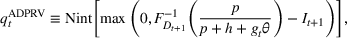
The ADPRV heuristic

Putting steps 1 and 2 together, our proposed heuristic, which we call the age‐dependent PRV (ADPRV), orders
$q_{t}^{ADPRV}$
at time t, which is defined as
$\begin{matrix} q_{t}^{ADPRV} \equiv Nint [\max (0, F_{D_{t + 1}}^{- 1} (\frac{p}{p + h + g_{t} θ}) - I_{t + 1})], \end{matrix}$
17where
$I_{t + 1}$
is given by (14), and
$g_{t}$
is given by
$g_{t} = (\frac{\sum_{i = 1}^{m} (ψ_{i} \prod_{v = 1}^{i - 1} {\hat{a}}_{t + v} (1 - ψ_{v}))}{\sum_{i = 1}^{m} (\prod_{v = 1}^{i - 1} {\hat{a}}_{t + v} (1 - ψ_{v}))})$
18for
${\hat{a}}_{t}$
defined in (16).

Comparison of the order quantities of NV, PRV, and ADPRV

In this subsection, we compare the three heuristics just introduced to each other and examine whether they underorder or overorder compared to optimal.

No on‐hand stock at t

First, we examine the simple case of the order at time t when the inventory is empty. Examination of their respective definitions in (10), (12), and (17) with
$x_{t} = 0$
shows that the orders of NV, ADPRV, and PRV are
$\begin{matrix} F_{D_{t + 1}}^{- 1} (\frac{p}{p + h + θ}) & \leq & F_{D_{t + 1}}^{- 1} (\frac{p}{p + h + g_{t} θ}) \\ \leq & F_{D_{t + 1}}^{- 1} (\frac{p}{p + h}), \end{matrix}$
19respectively. The inequalities follow from the fact that
$F_{D}^{- 1}$
is increasing for any random variable D, and
$g_{t}$
in (18) is between 0 and 1. Since PRV ignores outdating, it underestimates the expected lifetime cost of a new item, so overorders; on the other hand, NV optimally solves the problem where all items outdate, so underorders. In other words, like the order of ADPRV, the optimal order lies between the orders of NV and PRV. This behavior can be seen in Figure 1, which shows the three heuristics' orders and the optimal order as the total on‐hand stock varies for two closely related problems with
$m = 2$
.

FIGURE 1
Optimal and heuristic orders in period 1 by total period 1 stock for two problems with
$m = 2$
,
$T = 200$
,
$h = 1$
,
$ψ_{1} = 0.3$
,
$c = 5$
,
$γ = 0.999$
, and demand following a negative binomial distribution with parameters 5 and 0.8. For optimal and ADPRV, where the order amount depends on the individual ages of the stock, the average over all states with the same total stock is taken. In (a)
$p = 5, θ = 15$
, PRV > ADPRV for all states and in (b)
$p = 15, θ = 5$
, ADPRV > PRV for large stock.

Some on‐hand stock at t

Now we consider the general case where
$x_{t} \geq 0$
. First, consider NV. As (10) shows, NV orders the same amount no matter the value of
$x_{t}$
since all unsold product is assumed to perish. Further, NV orders less than optimal when
$x_{t} = 0$
and the optimal order must drop to 0 for large enough
$x_{t}$
. It follows that NV underorders when
$x_{t}$
is small and overorders when
$x_{t}$
is large enough, a pattern evident in Figure 1.

When
$x_{t} \geq 0$
, PRV simply subtracts the expected number of unsold items from its
$x_{t} = 0$
order. Therefore, as
$x_{t}$
increases, PRV's order monotonically decreases to 0. It follows that there exists y such that PRV orders more than NV if and only if
$x_{t} \leq y$
; see Figure 1. Ignoring outdating of current stock means PRV overestimates future stock levels, which encourages underordering. The significance grows with
$x_{t}$
, so, after overordering when
$x_{t} = 0$
, PRV leans more and more towards underordering as
$x_{t}$
increases. Figure 1 shows two cases. In Figure 1a, the optimal order hits 0 before PRV can start to underorder, while in Figure 1b PRV does underorder for large
$x_{t}$
until it hits 0.

Unlike PRV, (17) shows that ADPRV's order at time t depends not only on the total inventory
$x_{t}$
but also on its age distribution. Yet ADPRV still exhibits decreasing behavior in the sense that, for any
$i \in {1, …, m}$
, ADPRV's order will decrease if the age i stock increases and all other ages of stock stay the same. To help choose their time t order, both ADPRV and PRV estimate the expected on‐hand stock at time
$t + 1$
. Yet, since it does account for unsold items perishing, ADPRV's estimate is smaller. Therefore, if
$x_{t}$
grows by 1, no matter the age of the extra item, ADPRV's order will decrease by no more than PRV's. In other words, as
$x_{t}$
rises, ADPRV's order decreases less severely than PRV's, as Figure 1 shows.

Recall from (19) that ADPRV always orders less than PRV when
$x_{t} = 0$
. In some problems (e.g., Figure 1b but not Figure 1a), PRV catches ADPRV due to its steeper gradient, meaning there exist
$x_{t}$
where ADPRV's order is larger than PRV's. Such problems usually have large perish probabilities, causing a big difference between the estimated expected on‐hand stock at time
$t + 1$
of ADPRV and PRV and hence a big difference in gradients, or they have θ small compared to p, meaning that the orders of ADPRV and PRV are close when
$x_{t} = 0$
. While both problems in Figure 1 have the same perish probability,
$p / θ$
is small in Figure 1a but large in Figure 1b.

Further, Figure 1 shows ADPRV's order is close to optimal for all inventory levels, with a tendency to underorder more than overorder. Reasons behind this behavior will be discussed in Section 5 when the performance of ADPRV is analyzed.

Multi‐stage lookahead policies

In this subsection, we design heuristics which consider costs for a given number of future periods, but no further.

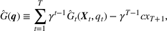
Recall
$J_{t} (x_{t}, q_{t})$
is the expected cost from period t until the terminal time T if at period t the state and order are x _t and
$q_{t}$
, and from period
$t + 1$
onwards the optimal order is made. The exact n ‐lookahead heuristic (En) orders
$\min_{q_{t}} (J_{\max (t, T - n)} (x_{t}, q_{t}))$
20at period t. In other words, if there are less than n periods to go, order to minimize the cost over all remaining periods (in which case the optimal order is made). Otherwise, if there are more than n periods to go, order to minimize the cost over the next n periods, assuming that all leftover inventory after these n periods is salvaged, so that the terminal cost summarizes the value of the remaining inventory.

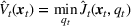
Clearly, the larger we choose n, the closer En will be to the optimal policy, but the greater the computational effort to calculate En. When the optimal policy requires too much computational effort to calculate, the largest n such that En is calculable can provide a good estimate of the optimal policy and hence a good benchmark for other, simpler heuristics.

The computation involved to calculate En can be reduced by assuming all items of age class i perish together with probability
$ψ_{i}$
, and otherwise none perish, in other words, solving our model with n periods but with dependent perishing as in Ketzenberg et al. (2015) replacing our usual independent perishing assumption. Since it is a heuristic for our setting with independent perishing, we call the solution to the model with this assumption the exact n‐lookahead heuristic with dependent perishing (En Dep).

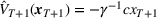
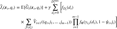
Another way to reduce the computational effort to calculate E1 specifically is to use Proposition 2, which shows that the remaining cost at period
$T - 1$
is convex in the order at
$T - 1$
. Since E1, aside from the last period, always assumes we are at period
$T - 1$
, convex optimization techniques can reduce its computational time.

NUMERICAL STUDY

We conduct an extensive numerical study. In Section 5.1, we describe the parameters used to generate data on which we assess our heuristics in Sections 5.2 and 5.3. We also analyze effects of the parameters on our leading heuristics' performance and show that dependent perishing is not always a good substitute for independent perishing. In Section 5.4, we examine the performance of the lower bound on the optimal cost. In Section 5.5, we apply our heuristics to real data from a large European retail company.

Experimental design

In this section, we choose parameters to reflect a wide variety of scenarios. A summary of the parameters is given in Table 2.

TABLE 2
Overview of parameters

Maximum lifetime (m) 2, 3, 4

Demand (D) Poisson(20), NegBin(5, 0.8), Unif(0,40)

Holding cost ( $\hat{h}$ ) 1

Order cost (c) 5

Penalty cost (
$\hat{p}$
) 10, 15, 20

Outdating cost (
$\hat{θ}$
) 0, 5, 10

We examine maximum lifetimes
$m = 2, 3$
, and 4. We expect the effect of an increasing lifetime to decrease because inventory is depleted according to a FIFO policy. Therefore, items with a high age class will mostly not be present. To investigate the effect of customer demand, we use three demand distributions with the same mean: a Poisson distribution with mean 20, which is close to symmetrical, a right‐skewed negative binomial distribution with parameters 5 and 0.8, and a discrete uniform distribution on [0,40]. These distributions have variances of 20, 100, and 400/3, respectively. Note that the first two distributions are more common in retailing, with the latter included for illustrative purposes.

Inventory holding costs
$\hat{h}$
are normalized to 1, and order cost c is set to 5. The cost of a shortage must be at least the selling price, which must be at least the order cost
$c = 5$
. Plus, there may be a loss of future sales due to loss of goodwill. Therefore, we examine
$\hat{p} = 10, 15, 20$
. The cost of outdating could be very small if the retailer is large and has efficient waste disposal. For smaller retailers, it could be a lot higher, so we examine
$\hat{θ} = 0, 5, 10$
.

We choose a high discount factor,
$γ = 0.999$
, to ensure costs over the entire time horizon of
$T = 200$
are reflected in the results. This means that the transformed parameter values from Proposition 1 are roughly
$h \approx 1$
;
$p \approx 5, 10, 15$
;
$θ \approx 5, 10, 15$
.

As illustrated in Table 3, we consider five distinct perish probability sets for each maximum lifetime. In each, the perish probabilities increase with age to reflect older products becoming more and more likely to perish. In total, we consider 135 settings.

TABLE 3
Perish probabilities for maximum lifetimes
$m = 2, 3, 4$

Maximum lifetime (m) Sets of perish probabilities ( $ψ_{1}, …, ψ_{m}$ )

2 (0.1), (0.2), (0.3), (0.4), (0.5)

3 (0.1, 0.2), (0.2, 0.3), (0.3, 0.4), (0.4, 0.5), (0.5, 0.6)

4
(0.1, 0.2, 0.3), (0.2, 0.3, 0.4), (0.3, 0.4, 0.5),

(0.4, 0.5, 0.6), (0.5, 0.6, 0.7)

Maximum lifetime
$m = 2$

For a maximum lifetime of
$m = 2$
, we can solve the model with
$T = 200$
optimally with dynamic programming and hence calculate the percentage increase from the optimal expected cost to the expected cost of each heuristic. Since the order costs incurred at the terminal time do not depend on the ordering policy, we omit them from the calculations to show the effect of each ordering policy separately. Results are shown in Table 4 with the perish probabilities for
$m = 2$
from Table 3 and parameters from Table 2. Further, a box plot showing the variability of the performance of each heuristic (except E3, which is so close to optimal) can be found in Figure 2a, and another showing E1 and ADPRV for different demand distributions can be found in Figure 2b.

TABLE 4
Percentage increase from optimal to heuristic expected cost for
$m = 2$
across different parameters

Parameter Value NV PRV ADPRV E1 Dep E1 E2 E3

Demand (D) Pois(20) 9.16 10.59 1.52 2.05 0.43 0.01 0.00

NB(5,0.8) 6.38 19.18 0.69 3.54 2.04 0.03 0.00

U(0,40) 8.35 17.30 0.11 4.44 3.06 0.22 0.00

Penalty cost ( $\hat{p}$ ) 10 7.90 24.84 0.53 2.18 1.85 0.04 0.00

15 6.30 13.26 0.81 3.27 1.89 0.09 0.00

20 9.70 8.96 0.98 4.57 1.81 0.13 0.00

Outdating cost (
$\hat{θ}$
) 0 10.20 4.06 0.69 3.67 1.24 0.11 0.00

5 5.98 14.96 0.79 3.20 1.95 0.08 0.00

10 7.71 28.05 0.84 3.16 2.36 0.06 0.00

Perish probability (ψ₁) (0.1) 18.44 11.38 2.27 7.65 5.53 0.26 0.01

(0.2) 10.19 13.25 0.84 4.20 2.15 0.11 0.00

(0.3) 5.88 15.56 0.46 2.52 0.95 0.04 0.00

(0.4) 3.41 17.97 0.21 1.46 0.42 0.02 0.00

(0.5) 1.90 20.28 0.09 0.88 0.18 0.01 0.00

Average 7.96 15.69 0.77 3.34 1.85 0.09 0.00

Standard deviation 9.39 14.30 1.35 3.39 2.81 0.19 0.00

Abbreviations: ADPRV, age‐dependent PRV; E1, E2, E3, exact lookahead heuristics; E1 Dep, exact lookahead heuristic with dependent perishing; NB, negative binomial distributions; NV, newsvendor heuristic; Pois, Poisson distributions; PRV, periodic review heuristic; U, uniform distributions.

FIGURE 2
Box plots showing the variability of heuristic performance for
$m = 2$
. Subfigure (a) shows all heuristics in Table 4 (except E3) against the optimal policy. Subfigure (b) shows E1 and ADPRV across the three different demand distributions, where “Po,” “NB,” and “U” stand for the Poisson, negative binomial, and uniform distributions detailed in Table 2.

NV and PRV, the most basic of our heuristics which are frequently applied in practice, can perform poorly, Figure 2 showing both can be as much as 60% above optimal. Further, Table 4 shows that, even for parameters where one of the two performs better, ADPRV or E1 is at least two times closer to optimal, often much more. This demonstrates that neglecting the effect of stochastic perishing can lead to substantial losses.

In a PRV model no product perishes, so PRV performs better the lower ψ₁. In addition, no perishing means the main cost to avoid is the penalty cost p; therefore, PRV stocks high to avoid product shortages. When p is high and θ is low, the optimal policy displays the same behavior, so PRV performs better. NV assumes that all product perishes, so performs better the larger ψ₁.

In the remainder of this section, we first focus on the differences between independent and dependent perishing and then compare across different parameters our two main heuristics, E1 and ADPRV.

Dependent versus independent perishing

On average, Table 4 shows that E1 Dep performs almost twice as badly as E1, suggesting a benefit in assuming products of the same age perish independently rather than all together as in Ketzenberg et al. (2015). Yet, in fact, the difference in order quantities between E1 and E1 Dep varies wildly from problem to problem. This effect is demonstrated in Figure 3, which shows, for four of our 135 problem settings, the orders of ADPRV, E1, and E1 Dep minus the optimal order quantity for different total on‐hand stock levels.

FIGURE 3
Difference between optimal and E1, E1 Dep, and ADPRV orders at period 1 by total period 1 on‐hand stock for
$m = 2$
,
$T = 200$
,
$h = 1$
, and
$c = 5$
. Note that p and θ are the same for each row.

In some problems, Figure 3d as an example, E1 and E1 Dep are virtually identical. Yet in others, for example, Figures 3a and 3b, E1 Dep begins to overorder compared to optimal once the total on‐hand stock surpasses the mean of the demand distribution (which is 20), with the size of the overorder growing with the inventory level up to a remarkable 20. In fact, no matter how large the total on‐hand stock levels become, E1 Dep still makes a nonzero order when the optimal, ADPRV and E1 orders are 0. We also see E1 Dep underorder compared to optimal by four items for medium on‐hand stock levels in Figure 3c. Below, we explain both behaviors.

First, we explain the overordering of E1 Dep seen in Figures 3a and 3b where
$p / θ$
is large. Suppose the state is
$x_{t} = (S, S)$
for large S. If S is large enough, all demand in period t will be covered by the age two stock, so S age one items will remain at the end of period t. The amount that will carry over to period
$t + 1$
follows a binomial distribution with parameters S and
$1 - ψ_{1}$
, and hence mean
$S (1 - ψ_{1})$
. If ψ₁ is not too large, we can take S large enough so that the optimal order at time t is 0, since so much age one product is likely to carry over. Since E1 and ADPRV assume the above independent perishing model, their order is also 0 for large S.

If perishing was dependent instead, S age one products would survive to period
$t + 1$
with probability
$(1 - ψ_{1})$
, and 0 would survive with probability ψ₁. When p is large compared to θ, E1 Dep, which assumes dependent perishing, desperately wants to avoid having no product at all at time
$t + 1$
to avoid a large penalty cost, so, at the expense of risking a smaller outdating cost in the future, makes a large order at time t in case all S on‐hand items perish before
$t + 1$
. In reality with independent perishing, for large S the chance of all or most of the S age one items perishing is negligible, so the retailer is not actually at much risk of incurring penalty costs at time
$t + 1$
at all if they order 0. In other words, E1 Dep orders high to safeguard against a scenario which, in real life, is extremely unlikely to happen.

The underordering of E1 Dep in Figure 3c occurs because E1 Dep starts to order 0 just after the total stock exceeds 40, while the optimal policy waits until around 65. The reason for this difference is linked both to a small
$p / θ$
and, just like the overordering case, E1 Dep anticipating a situation likely to happen with dependent perishing, but very unlikely with independent perishing. This time, the situation is none of a large number of on‐hand items perish, so newly ordered stock will not be sold. Any unsold item risks a perishing cost θ; since θ is large compared to p, E1 Dep orders nothing much sooner than the optimal policy as total stock levels rise.

To summarize, while in some settings the retailer will perform just as well assuming a simpler dependent perishing model, in others, particularly when there is a large difference between penalty and outdating costs, this assumption will achieve very poor results, with the retailer at risk of either over‐ or underordering compared to optimal.

E1 versus ADPRV

While the lookahead heuristics E2 and particularly E3 perform excellently, their computational complexity prevents their practical use. In this section, we compare our two leading practical heuristics, E1 and ADPRV.

On average, ADPRV performs better than E1, as can be seen from Table 4 and Figure 2a. ADPRV also has a smaller standard deviation than E1, showing a more steady performance over a wide range of parameters. Yet, there are problem settings where E1 beats ADPRV and hence should be preferred. In this subsection, we shall explain the patterns in performance concerning demand and perish probability that lead to these preferences and examine the ordering bias of both heuristics.

Demand and perish probability

Both E1 and ADPRV perform better the larger ψ₁, since the problem is easier to solve: the more items that perish, the higher the proportion of the inventory level at the next period that is made up of the retailer's order, a quantity over which the retailer has complete control. When
$ψ_{1} = 1$
, they both reduce to NV which is optimal in this case.

As for demand, E1, which looks ahead just one period, performs well for Poisson, since there is low variance in demand from period to period, so the next period is more representative of general behavior. As the variance of demand increases from the Poisson to the negative binomial to the uniform, the next period becomes less representative and, as shown in Figure 2b, E1's performance worsens.

Figure 2b also shows that ADPRV, on the other hand, thrives when demand variance is high. The cause, explained in the following, is due to an effect also linked to the perish probability. ADPRV calculates its order by simply taking the expectation over both demand and perishing for the next period. The optimal policy is more bespoke, taking into account the whole distribution of demand and perishing, in both the next and future periods. When the variance of demand or perishing (or both) increases, the expectations used by ADPRV will be less accurate, so the cost under ADPRV will rise. However, the cost under the optimal policy will rise by a greater amount, since its more advanced toolkit, which is of great use when demand and perishing are more certain, becomes less and less advantageous over simply using the expectation as ADPRV does. In other words, the optimality gap of ADPRV decreases when the level of uncertainty in either demand or perishing (or both) rises. As Table 5 shows, the optimal policy shows a strong improvement on ADPRV's crude approach only when there is low uncertainty both in demand (Poisson) and perishing (low ψ₁).

TABLE 5
ADPRV and E1 performance over subsets of problem instances

$m = 2$
$m = 3$

$m = 4$

Demand ψ₁ ADPRV E1 ADPRV E1 ADPRV E1

Poisson 0.1,0.2,0.3 2.40 0.59 0.68 0.52 0.61 0.52

Poisson 0.4,0.5 0.18 0.19 0.13 0.18 0.14 0.18

Non‐Poisson 0.1,0.2,0.3 0.58 4.02 0.32 1.27 0.27 1.04

Non‐Poisson 0.4,0.5 0.13 0.36 0.05 0.20 0.06 0.21

Abbreviations: ADPRV, age‐dependent PRV; E1, exact 1‐lookahead heuristic; PRV, periodic review heuristic.

E1, like the optimal policy, also uses the whole distribution of demand and perishing but only for the next period, which is sufficient for good performance when uncertainty is low. As a result, Table 5 shows that E1's advantage over ADPRV is only for both small ψ₁ and Poisson demand.

Bias in the order quantities

Figure 3 demonstrates that both E1 and ADPRV have some ordering bias, the former (respectively, latter) tending to consistently order more (respectively, less) than the optimal policy.

E1 chronically overorders since it assumes all product which survives to age 2 is salvaged at its order cost. In reality, if such product does not sell at age 2, it perishes for cost θ. The resulting overordering will be punished more severely the larger the outdating cost θ, explaining why E1 degrades with the outdating cost θ in Table 4.

Figure 3 also shows that the overordering of E1 is more pronounced for the negative binomial and uniform distributions, as the more unpredictable demand is, the more likely a product is to remain unsold for its entire lifetime and hence perish after two periods, a cost which E1 does not consider. Further, it can be seen from Figure 3 that the overordering effect is worse for smaller ψ₁, since the smaller ψ₁ is the greater the proportion of total product perishing that occurs at age 2.

Figure 3 shows that ADPRV usually underorders. For example, in Figure 3d, where
$p / θ$
is low, ADPRV underorders when there is no stock, in which case its order is
$F_{D_{t + 1}}^{- 1} (\frac{p}{p + h + g_{t} θ}),$
21which balances underage and overage costs. This effect occurs because, while the underage cost, p, is known, the overage cost is estimated by ADPRV using
$g_{t}$
(defined in (18)), which accounts for the probability of an overordered item perishing at some point in its lifetime. Numerical investigation suggests
$g_{t}$
tends to slightly overestimate the overage cost,
$h + g_{t} θ$
. The smaller
$p / θ$
the more influence
$g_{t}$
has on (21), so the more likely ADPRV is to underorder when there is no stock.

In Figures 3a, 3b and 3d, ADPRV's underordering generally grows with the on‐hand stock until it becomes large enough for both ADPRV and the optimal policy to order 0. We see this behavior for the following reason. No matter the current inventory, ADPRV orders at time t with the aim for the on‐hand stock to be (21) at time
$t + 1$
. However, the larger
$x_{t}$
, the larger the ratio of old to new stock in the time
$t + 1$
inventory. Older stock has less value than newly ordered stock due to a higher chance of perishing sooner; therefore, the larger
$x_{t}$
, the more likely (21) is to be below the optimal time
$t + 1$
on‐hand‐stock level.

We do not see the above effect in Figure 3c for two reasons. First, ψ₁ is larger, so items are less likely to survive to age 2, meaning the old to new stock ratio at time
$t + 1$
is smaller. Second, ADPRV calculates its time t order using only expected values, ignoring the uncertainty arising from demand and perishing at time t. Due to this uncertainty, the optimally ordering retailer slightly biases their order away from the expected values to avoid the heaviest cost. In Figure 3c, the outdating cost is dominant, so the optimal policy orders a little less than the expected values, which counteracts ADPRV's underordering tendencies.

Maximum lifetime
$m = 3, 4$

Due to the large number of states, problems with maximum lifetimes greater than 2 cannot be optimally solved by dynamic programming, so neither optimal nor heuristic expected costs can be calculated. Therefore, for
$m = 3, 4$
, we use simulation to estimate costs under each heuristic. For each parameter setting, we simulate 10,000 runs with
$T = 200$
, with run length chosen by comparing the average simulated heuristic cost to the expected heuristic cost when
$m = 2$
. The furthest computationally tractable lookahead heuristic is E3 for
$m = 3$
and E2 for
$m = 4$
, both shown to be close to optimal when
$m = 2$
. Yet, the average percentage decrease in costs from E2 to E3 for
$m = 3$
is only 0.01%. Therefore, to make the
$m = 3$
and
$m = 4$
results comparable, we benchmark both using E2.

Results are shown in Table 6 for
$m = 3$
, with the corresponding perish probabilities from Table 3 and parameters from Table 2. The results for
$m = 4$
are very similar, so are presented in Table EC.5 in Supporting Information Section EC.5. Such similarity implies that most products are either sold or perished before reaching a high age class, as in accordance with the FIFO depletion policy. For both
$m = 3$
and 4, box plots showing similar patterns to those in Figure 2 for
$m = 2$
can be found in Supporting Information Section EC.6.

TABLE 6
Percentage increase from the benchmark (E2) to heuristic cost over 10,000 runs for
$m = 3$
across different parameters

Parameter Value NV PRV ADPRV E1 Dep E1

Demand (D) Pois(20) 9.83 10.52 0.46 1.93 0.38

NB(5,0.8) 9.19 14.56 0.27 1.65 0.65

U(0,40) 14.51 11.52 0.13 2.17 1.02

Penalty cost ( $\hat{p}$ ) 10 9.71 20.01 0.12 1.00 0.69

15 9.27 9.99 0.26 1.87 0.70

20 14.56 6.60 0.48 2.87 0.65

Outdating cost (
$\hat{θ}$
) 0 15.58 3.20 0.36 2.55 0.53

5 8.09 11.36 0.25 1.74 0.70

10 9.87 22.04 0.26 1.46 0.80

Perish probabilities (
$ψ_{1}, ψ_{2}$
) (0.1,0.2) 28.49 4.43 0.80 3.28 1.70

(0.2,0.3) 13.95 8.51 0.30 2.49 0.84

(0.3,0.4) 7.36 12.57 0.18 1.84 0.49

(0.4,0.5) 3.98 16.20 0.10 1.19 0.26

(0.5,0.6) 2.11 19.29 0.05 0.78 0.12

Average 11.18 12.20 0.29 1.92 0.68

Standard deviation 14.62 12.52 0.46 1.49 0.75

Abbreviations: ADPRV, age‐dependent PRV; E1, E2, exact lookahead heuristics; E1 Dep, exact lookahead heuristic with dependent perishing; NB, negative binomial distributions; NV, newsvendor heuristic; Pois, Poisson distributions; PRV, periodic review heuristic; U, uniform distributions.

NV and PRV can again both perform poorly compared to the other heuristics, but, as expected, NV (which assumes
$m = 1$
) gets worse as m increases from 2 to 3, and PRV (which assumes
$m = \infty$
and no perishing) gets better. In fact, the performance of all heuristics except NV improves as m increases from 2 to 3, since inventory lasts longer, so the retailer has more opportunity to correct an under‐ or overorder in a previous period. NV orders independently of the current stock level, so does not share this benefit.

The difference in performance between E1 and E1 Dep increases with m since there are more opportunities for products to perish, a process for which E1 and E1 Dep have different underlying assumptions. E1 is around three times better than E1 Dep when
$m = 3$
.

Similarly to
$m = 2$
, Table 6 shows that ADPRV does better when demand is more varied and E1 better when demand is less varied when
$m = 3$
, but Table 5 shows it is in the combination of Poisson demand and low perish probabilities where E1's whole advantage lies. Based on these findings, we suggest that the retailer assesses both demand variability and perish probabilities. If demand variability and perish probabilities are both low, choose E1, because there are significant benefits to E1's use of the whole distributions of demand and perishing, and one period is fairly representative of the rest so there is not much benefit to looking ahead any further. Otherwise, choose ADPRV, since the more thorough analysis of E1 (which also adds computational complexity) is not as useful, and, since demand is more varied, it is important to consider perishing costs several time periods ahead.

Lower bound on optimal cost

Recall that for
$m \geq 3$
the optimal cost is computationally intractable with
$T = 200$
and our choice of demand distributions with mean 20. While E2 provides a very tight upper bound, E2's computational complexity grows sharply with m due to the exponential growth of the state space. In our numerical study, calculating E2 for a single problem case for
$m = 4$
typically takes between 24 and 72 hours.

To quickly approximate the optimal cost for problems with larger m, we turn to the lower bound discussed in Section 3, which solves the problem where the perish probability for all ages is
$ψ \equiv \min_{i = 1, …, m} ψ_{i}$
. The resulting state space is simply the total inventory, so computational complexity is low and unaffected by an increase in m.

In this section, we test the lower bound by calculating the percentage decrease from the benchmark cost to the lower bound for
$m = 2, 3$
, and 4. As before, the benchmark is the optimal expected cost for
$m = 2$
and the simulated E2 cost for
$m = 3$
and 4. Table 7 shows the results, both overall and split by demand distribution or ψ₁ value.

TABLE 7
Percentage decrease from benchmark to lower bound for
$m = 2, 3, 4$
across different demand distributions and age 1 perish probabilities

Pois(20) NB(5,0.8) U(0,40) $ψ_{1} \in {0.1, 0.2}$
$ψ_{1} \in {0.3, 0.4, 0.5}$
Overall

$m = 2$
−0.14 −3.66 −8.53 −8.10 −1.45 −4.11

$m = 3$
−0.07 −0.92 −2.94 −2.72 −0.37 −1.31

$m = 4$
−0.05 −0.91 −2.99 −2.79 −0.34 −1.31

Abbreviations: NB, negative binomial distributions; Pois, Poisson distributions; U, uniform distributions.

We see a clear improvement from
$m = 2$
to
$m = 3, 4$
, a useful trait since
$m = 3, 4$
is where the bound is most needed. Recall that the uniform distribution is included in our numerical study for illustrative purposes and not for any relevance to retailing. In the realistic cases of Poisson and negative binomial, the lower bound is within 0.5% of optimal on average for
$m = 3$
and 4. However, Table 7 shows that the lower bound performs much better in some problem instances than others.

To explain these patterns, note that the perish probabilities in Table 3 used in our numerical study increase with age. Therefore, the perish probability used for all ages by the lower bound satisfies
$ψ \equiv \min_{i = 1, …, m} ψ_{i} = ψ_{1}$
, which becomes less accurate as product age increases. When either ψ₁ is large or demand is less variable, product is less likely to survive until these badly estimated older ages, so the better the lower bound performs.

Perish probabilities also explain the improvement in the lower bound with m. The most inaccurately estimated perish probability is the mth, where the lower bound model is out by
$1 - ψ_{1}$
. As m increases, the significance of this large inaccuracy decreases, since by FIFO product becomes less and less likely to remain in the inventory the older it becomes. This explains a lower bound tighter for
$m = 3, 4$
than
$m = 2$
, but we would also expect to see the lower bound tighter for
$m = 4$
than
$m = 3$
. However, the results are almost identical because so few products make it to age 3 that there is little benefit to the better approximation of the third perish probability when
$m = 4$
.

Real data

We compare our leading heuristics E1 and ADPRV both to each other and to the basic heuristics NV and PRV using real data from a large European retail company to better understand their performance in practice. We consider different types of perishable products (fruit and vegetables) that have different maximum lifetimes and perishability patterns. Table 8 contains the perish probabilities of the products, which start from 0.3 or 0.4 for the first day, and increase or stay the same for the days thereafter, reaching 1 by a maximum of 8 days. At the end of the day, the store manager checks which items are still salable for the next day and can be carried over. All perished items are discarded. The managers use their own judgment to place an order for the next day.

TABLE 8
Perish probabilities

Perish probability at the end of each day

Product Max. lifetime Day 1 Day 2 Day 3 Day 4 Day 5 Day 6 Day 7 Day 8

Mushrooms 2 days 0.3 1

Blueberries 5 days 0.4 0.5 0.6 0.8 1

Broccoli 5 days 0.3 0.3 0.4 0.8 1

Pineapples 4 days 0.3 0.3 0.5 1

Apples 8 days 0.3 0.3 0.3 0.3 0.3 0.3 0.3 1

We evaluate these products with sales data of 66 stores. We collected daily selling prices and current batch sizes for each date, since the retailer can only order products in given batch sizes. Shortage penalty costs consist of the difference between selling price and ordering costs adjusted with discount factor
$γ = 0.999$
, the latter chosen to ensure that costs over the entire time horizon are reflected in the results. Due to confidentiality reasons, we normalize the data so shortage penalty costs equal one. The daily unit inventory holding cost rates are 0.25% of the penalty costs. The outdating cost equals the penalty cost multiplied by 1.12 to reflect the cost of a lost sale in addition to disposal and handling costs of the outdated item. For each product–store combination, we have over 500 days of data.

Since we are only able to collect sales data and lost sales are unobserved, we estimate demand using hourly sales data and product‐ and store‐specific demand patterns based on the nonparametric approach developed by Lau and Lau (1996). We assume that demand is Poisson‐distributed and forecast demand with rolling‐horizon Poisson regression. As external variables, we consider lagged demand, selling price, and weekdays. Note that we can only consider a time lag of greater than 1 day since the last day's sales are not yet known when the order decision is made.

Results are shown in Table 9. Overall 321 product–store combinations, as expected since demand is Poisson, E1 performs the best and is hence used to benchmark the other three heuristics. NV performs very badly on average, with PRV a substantial improvement. However, the standard deviation of PRV is higher than NV, showing that there are scenarios where PRV can perform just as badly as NV. Indeed, in their worst‐case scenarios, NV and PRV have costs 23.8% and 22.8% higher than E1, respectively.

TABLE 9
Average and standard deviation of NV, PRV, and ADPV expressed as percentages over E1 for 321 product–store combinations

NV over E1 PRV over E1 ADPRV over E1

Average 14.8% 4.4% 0.45%

Standard deviation 4.17% 4.83% 1.08%

Abbreviations: ADPRV, age‐dependent PRV; E1, exact lookahead heuristic order; NV, newsvendor heuristic; PRV, periodic review heuristic.

On average, the performance of ADPRV is close to E1 without much variation. In its best‐case scenario, ADPRV has costs 2.1% lower than E1, and in its worst case costs 4.6% higher. Therefore, choosing E1 over ADPRV or vice versa does not make much of a difference to the retailer's costs, and, with its reduced computational complexity, ADPRV may well be preferable.

CONCLUSION

We develop a periodic review inventory control model with stochastic demand and perishing, lost sales, and a FIFO depletion policy where the perish probability depends on the age class of the product. The novelty of our model is that we allow products to perish independently of one another. This is an important feature not only because of its practical relevance (one bad product rarely spoils the whole bunch) but also because we find significant differences in ordering patterns compared to the dependent perishing assumption of Ketzenberg et al. (2015). Consequently, assuming dependent perishing can lead to poor performance if products perish independently in reality.

We construct an MDP and show that convexity holds in the penultimate period, but, via a simple counterexample, that convexity can fail any earlier. In addition to an optimal solution algorithm, we also develop two new heuristic policies which find excellent solutions to large problem instances that cannot be solved optimally due to the curse of dimensionality. The first is a combination of the optimal solutions to the well‐known newsvendor and periodic review models, and the second is a one‐stage lookahead policy.

Using simulated data and data from a large European retail chain, we show that our heuristics outperform existing models, which do not fully consider the characteristics of the perishing process. This research also provides important practical insights. The retail chain initially considered using commercial software solutions that contain standard methods such as NV and PRV. However, our research clearly indicates that they would be better off using the new E1 and ADPRV heuristics presented in this paper. In a thorough comparison of E1 and ADPRV, we explain their performance patterns arising in our numerical study. In particular, we highlight that, for problem parameters where one heuristic shows weaker performance, the other shows a stronger performance. Therefore, our results can advise retailers which heuristic to use depending on the nature of the demand they receive and the perish probabilities of the products they sell.

In our model, we assume a FIFO approach that corresponds to common stocking policies of retailers. It would also be interesting to analyze a LIFO approach or a mixture of approaches to account both for different stocking policies and customers that pick the freshest products from behind. Another important aspect in retailing is the multiechelon structure, where the supply chain consists of suppliers, distribution centers, and/or warehouses from which products are delivered to multiple stores. A multiechelon inventory policy would require making order decisions at the different echelons and considering their interdependencies. For example, if the warehouse does not have enough stock to supply all orders, the policy would require shortage allocation rules or transshipments between stores could be used to better balance inventories. We leave these investigations to future research.

Footnotes
ACKNOWLEDGMENTS
We thank the department editor Jayashankar Swaminathan, the senior editor, and the anonymous referees for their constructive comments to improve the paper. The authors are grateful for the support of the EPSRC‐funded EP/L015692/1 STOR‐i Centre for Doctoral Training.
ORCID iD
Jake Clarkson
Anna‐Lena Sachs
Ulrich W. Thonemann
References
1.
Axsäter S. (2015). Inventory control. International Series in Operations Research & Management Science, Vol. 225. Springer.
2.
Bakker M. Riezebos J. Teunter R. H. (2012). Review of inventory systems with deterioration since 2001. European Journal of Operational Research, 221(2), 275–284.
3.
Chao X. Gong X. Shi C. Yang C. Zhang H. Zhou S. X. (2018). Approximation algorithms for capacitated perishable inventory systems with positive lead times. Management Science, 64(11), 5038–5061.
4.
Chao X. Gong X. Shi C. Zhang H. (2015). Approximation algorithms for perishable inventory systems. Operations Research, 63(3), 585–601.
5.
Chen S. Li Y. Zhou W. (2019). Joint decisions for blood collection and platelet inventory control. Production and Operations Management, 28(7), 1674–1691.
6.
Duan Q. Liao T. W. (2013). A new age‐based replenishment policy for supply chain inventory optimization of highly perishable products. International Journal of Production Economics, 145(2), 658–671.
7.
Goyal S. K. Giri B. C. (2001). Recent trends in modeling of deteriorating inventory. European Journal of Operational Research, 134(1), 1–16.
8.
Haijema R. Minner S. (2016). Stock‐level dependent ordering of perishables: A comparison of hybrid base‐stock and constant order policies. International Journal of Production Economics, 181, 215–225.
9.
Haijema R. Minner S. (2019). Improved ordering of perishables: The value of stock‐age information. International Journal of Production Economics, 209, 316–324.
10.
Haijema R. van derWal J. vanDijk N. M. (2007). Blood platelet production: Optimization by dynamic programming and simulation. Computers & Operations Research, 34(3), 760–779.
11.
Janssen L. Claus T. Sauer J. (2016). Literature review of deteriorating inventory models by key topics from 2012 to 2015. International Journal of Production Economics, 182, 86–112.
12.
Karaesmen, I. Z., Scheller‐Wolf, A., & Deniz, B. (2011). Managing perishable and aging inventories: Review and future research directions. In Kempf, K., Keskinocak, P., & Uzsoy, R. (Eds.), Planning production and inventories in the extended enterprise (chap. 15, pp. 393–436). Springer.
13.
Ketzenberg M. Bloemhof J. Gaukler G. (2015). Managing perishables with time and temperature history. Production and Operations Management, 24(1), 54–70.
14.
Kiesmüller G. P. Inderfurth K. (2018). Approaches for periodic inventory control under random production yield and fixed setup cost. OR Spectrum, 40(2), 449–477.
15.
Kouki C. Jouini O. (2015). On the effect of lifetime variability on the performance of inventory systems. International Journal of Production Economics, 167, 23–34.
16.
Lau H.‐S. Lau A. H.‐L. (1996). Estimating the demand distributions of single‐period items having frequent stockouts. European Journal of Operational Research, 92(2), 254–265.
17.
Minner S. Transchel S. (2010). Periodic review inventory‐control for perishable products under service‐level constraints. OR Spectrum, 32(4), 979–996.
18.
Nahmias S. (1975). Optimal ordering policies for perishable inventory—II. Operations Research, 23(4), 735–749.
19.
Nahmias S. (1976). Myopic approximations for the perishable inventory problem. Management Science, 22(9), 1002–1008.
20.
Nahmias S. (1977). On ordering perishable inventory when both demand and lifetime are random. Management Science, 24(1), 82–90.
21.
Nahmias S. (1982). Perishable inventory theory: A review. Operations Research, 30(4), 680–708.
22.
Nahmias, S. (2011). Perishable inventory systems. International Series in Operations Research & Management Science, Vol. 160. Springer Science & Business Media.
23.
Nahmias S. Pierskalla W. P. (1973). Optimal ordering policies for a product that perishes in two periods subject to stochastic demand. Naval Research Logistics Quarterly, 20(2), 207–229.
24.
Nandakumar P. Morton T. E. (1993). Near myopic heuristics for the fixed‐life perishability problem. Management Science, 39(12), 1490–1498.
25.
Reiner G. Teller C. Kotzab H. (2013). Analyzing the efficient execution of in‐store logistics processes in grocery retailing—The case of dairy products. Production and Operations Management, 22(4), 924–939.
26.
Sarhangian V. Abouee‐Mehrizi H. Baron O. Berman O. (2018). Threshold‐based allocation policies for inventory management of red blood cells. Manufacturing & Service Operations Management, 20(2), 347–362.
27.
Sonntag D. Kiesmüller G. P. (2017). The influence of quality inspections on the optimal safety stock level. Production and Operations Management, 26(7), 1284–1298.
28.
Van Zyl, G. (1964). Inventory control for perishable commodities [Ph.D. thesis]. University of North Carolina, Chapel Hill, NC.
29.
Voelkel M. A. Sachs A.‐L. Thonemann U. W. (2020). An aggregation‐based approximate dynamic programming approach for the periodic review model with random yield. European Journal of Operational Research, 281(2), 286–298.
30.
Williams C. L. Patuwo B. (1999). A perishable inventory model with positive order lead times. European Journal of Operational Research, 116(2), 352–373.
31.
Yano C. A. Lee H. A. (1995). Lot sizing with random yield: A review. Operations Research, 43, 311–334.
Supplementary Material
Please find the following supplemental material available below.
For Open Access articles published under a Creative Commons License, all supplemental material carries the same license as the article it is associated with.
For non-Open Access articles published, all supplemental material carries a non-exclusive license, and permission requests for re-use of supplemental material or any part of supplemental material shall be sent directly to the copyright owner as specified in the copyright notice associated with the article.
0.00 MB
0.57 MB

t	x _t	$q_{t}$	$d_{t}$	y _t	Perished units
1	(4,3,5)	7	4	(4,3,1)	(2,0,1)
2	(7,2,3)	9	6	(6,0,0)	(1,0,0)
3	(9,5,0)	4	15	(0,0,0)	(0,0,0)

Maximum lifetime (m)	2, 3, 4
Demand (D)	Poisson(20), NegBin(5, 0.8), Unif(0,40)
Holding cost ( $\hat{h}$ )	1
Order cost (c)	5
Penalty cost ( $\hat{p}$ )	10, 15, 20
Outdating cost ( $\hat{θ}$ )	0, 5, 10

Parameter	Value	NV	PRV	ADPRV	E1 Dep	E1	E2	E3
Demand (D)	Pois(20)	9.16	10.59	1.52	2.05	0.43	0.01	0.00
	NB(5,0.8)	6.38	19.18	0.69	3.54	2.04	0.03	0.00
	U(0,40)	8.35	17.30	0.11	4.44	3.06	0.22	0.00
Penalty cost ( $\hat{p}$ )	10	7.90	24.84	0.53	2.18	1.85	0.04	0.00
	15	6.30	13.26	0.81	3.27	1.89	0.09	0.00
	20	9.70	8.96	0.98	4.57	1.81	0.13	0.00
Outdating cost ( $\hat{θ}$ )	0	10.20	4.06	0.69	3.67	1.24	0.11	0.00
	5	5.98	14.96	0.79	3.20	1.95	0.08	0.00
	10	7.71	28.05	0.84	3.16	2.36	0.06	0.00
Perish probability (ψ₁)	(0.1)	18.44	11.38	2.27	7.65	5.53	0.26	0.01
	(0.2)	10.19	13.25	0.84	4.20	2.15	0.11	0.00
	(0.3)	5.88	15.56	0.46	2.52	0.95	0.04	0.00
	(0.4)	3.41	17.97	0.21	1.46	0.42	0.02	0.00
	(0.5)	1.90	20.28	0.09	0.88	0.18	0.01	0.00
Average		7.96	15.69	0.77	3.34	1.85	0.09	0.00
Standard deviation		9.39	14.30	1.35	3.39	2.81	0.19	0.00

		$m = 2$		$m = 3$		$m = 4$
Demand	ψ₁	ADPRV	E1	ADPRV	E1	ADPRV	E1
Poisson	0.1,0.2,0.3	2.40	0.59	0.68	0.52	0.61	0.52
Poisson	0.4,0.5	0.18	0.19	0.13	0.18	0.14	0.18
Non‐Poisson	0.1,0.2,0.3	0.58	4.02	0.32	1.27	0.27	1.04
Non‐Poisson	0.4,0.5	0.13	0.36	0.05	0.20	0.06	0.21

Parameter	Value	NV	PRV	ADPRV	E1 Dep	E1
Demand (D)	Pois(20)	9.83	10.52	0.46	1.93	0.38
	NB(5,0.8)	9.19	14.56	0.27	1.65	0.65
	U(0,40)	14.51	11.52	0.13	2.17	1.02
Penalty cost ( $\hat{p}$ )	10	9.71	20.01	0.12	1.00	0.69
	15	9.27	9.99	0.26	1.87	0.70
	20	14.56	6.60	0.48	2.87	0.65
Outdating cost ( $\hat{θ}$ )	0	15.58	3.20	0.36	2.55	0.53
	5	8.09	11.36	0.25	1.74	0.70
	10	9.87	22.04	0.26	1.46	0.80
Perish probabilities ( $ψ_{1}, ψ_{2}$ )	(0.1,0.2)	28.49	4.43	0.80	3.28	1.70
	(0.2,0.3)	13.95	8.51	0.30	2.49	0.84
	(0.3,0.4)	7.36	12.57	0.18	1.84	0.49
	(0.4,0.5)	3.98	16.20	0.10	1.19	0.26
	(0.5,0.6)	2.11	19.29	0.05	0.78	0.12
Average		11.18	12.20	0.29	1.92	0.68
Standard deviation		14.62	12.52	0.46	1.49	0.75

	Pois(20)	NB(5,0.8)	U(0,40)	$ψ_{1} \in {0.1, 0.2}$	$ψ_{1} \in {0.3, 0.4, 0.5}$	Overall
$m = 2$	−0.14	−3.66	−8.53	−8.10	−1.45	−4.11
$m = 3$	−0.07	−0.92	−2.94	−2.72	−0.37	−1.31
$m = 4$	−0.05	−0.91	−2.99	−2.79	−0.34	−1.31

		Perish probability at the end of each day
Product	Max. lifetime	Day 1	Day 2	Day 3	Day 4	Day 5	Day 6	Day 7	Day 8
Mushrooms	2 days	0.3	1
Blueberries	5 days	0.4	0.5	0.6	0.8	1
Broccoli	5 days	0.3	0.3	0.4	0.8	1
Pineapples	4 days	0.3	0.3	0.5	1
Apples	8 days	0.3	0.3	0.3	0.3	0.3	0.3	0.3	1

The periodic review model with independent age‐dependent lifetimes

Abstract

Keywords

INTRODUCTION

LITERATURE REVIEW

Fixed lifetime

Random lifetime

Random yield

MODEL

Sequence of events

Inventory transition

Total cost

HEURISTIC POLICIES

Newsvendor heuristic

Periodic review heuristic

A combination of NV and PRV

1. Expected on‐hand stock at t + 1 $t+1$

2. Order if on‐hand stock at t + 1 $t+1$ was known.

The ADPRV heuristic

Comparison of the order quantities of NV, PRV, and ADPRV

No on‐hand stock at t

Some on‐hand stock at t

Multi‐stage lookahead policies

NUMERICAL STUDY

Experimental design

Maximum lifetime m = 2 $m=2$

Dependent versus independent perishing

E1 versus ADPRV

Demand and perish probability

Bias in the order quantities

Maximum lifetime m = 3 , 4 $m=3,4$

Lower bound on optimal cost

Real data

CONCLUSION

Footnotes

ACKNOWLEDGMENTS

ORCID iD

References

Supplementary Material

1. Expected on‐hand stock at
$t + 1$

2. Order if on‐hand stock at
$t + 1$
was known.

Maximum lifetime
$m = 2$

Maximum lifetime
$m = 3, 4$