Dynamic stochastic lot sizing with forecast evolution in rolling‐horizon planning

Abstract

Academic approaches considering demand uncertainty in lot sizing are seldom used in practice. Industry typically implements deterministic models and accounts for uncertainties by using a rolling‐horizon planning framework with frequent forecast updates. This paper bridges this gap by proposing a stochastic lot‐sizing methodology adapted to rolling‐horizon processes. Using the martingale model of forecast evolution (MMFE), we are able to anticipate the forecast updates from rolling‐horizon planning in stochastic lot sizing. Our formulation is extended with production recourse to reflect the replanning flexibility of rolling‐horizon planning. Extensive simulations on both synthetic and real‐world data show the value of forecast evolution models. Forecast evolution models reduce actual costs by 14% on average compared to traditional deterministic planning. The advantage of the extended model with production recourse depends on several factors including capacity, correlation, and uncertainty. Sensitivity analyses show that recourse can reduce costs by an additional 3% on average and up to 10% in specific settings. Using real‐world and synthetic data, we provide the first analysis of the value of additive and multiplicative MMFE‐based planning models when the true forecast evolution process is unknown. We show that, contrary to the existing consensus, the additive model performs more robustly than the multiplicative model on a wide array of problem settings.

INTRODUCTION

Demand uncertainty has been studied extensively in stochastic lot sizing using probability distributions to model the uncertain demand. However, the use of these models in industry has been limited. A major shortcoming is that they cannot be integrated properly into the periodic planning processes that manufacturing companies use to update demand forecasts. Thus, the substantial information technology (IT) support, human resources, and time dedicated to forecasting are ignored. In fact, previous research on stochastic lot sizing has neglected the value of forecasts in generating demand distributions altogether. Stochastic lot‐sizing approaches suitable for industry adoption should exploit the data contained in historic forecasts. Demand distributions must be updated dynamically based not only on the latest demand realizations but also on forecasts to fit rolling‐horizon processes.

The use of forecast evolution models can bridge between stochastic lot‐sizing models and rolling‐horizon planning in industry. Different from demand distributions used in traditional stochastic lot sizing, they model demand uncertainty as encountered in rolling‐horizon planning. The martingale model of forecast evolution (MMFE) developed by Graves et al. (1986) and Heath and Jackson (1994) models future forecast changes as a stochastic process. Two methods for modeling the forecast evolution process according to the MMFE have been proposed. The additive model measures the difference between successive forecasts and assumes that these differences follow a multivariate normal distribution. The multiplicative model measures the ratio between successive forecasts and assumes that this ratio follows a log‐normal distribution. While it has been argued that the multiplicative model is more relevant when demand fluctuates over time (Hausman, 1969; Heath & Jackson, 1994), extensive comparisons of the two MMFE models are still missing. In particular, the cost of modeling error, that is using the additive or multiplicative model when the true process is unknown, has not been evaluated so far. Hence, MMFE models can be estimated directly from the history of past demand and successive forecasts revisions routinely collected in industry.

Demand forecasting is typically an organizational alignment step that is part of the sales and operations planning processes. Hence, the forecasts observed in each planning period can be a mix of expert judgmental forecasts and forecasts obtained from forecasting algorithms. Chen and Lee (2009) review how the MMFE generalizes several classical prediction models such as autoregressive moving average models. Here, the MMFE parameters can be determined exactly. Still, the strength of MMFE lies in its ability to integrate a combination of model‐based quantitative forecasts and expert‐based judgmental forecasts (Heath & Jackson, 1994). In this context, MMFE model parameters have to be estimated from historical data. Yet, despite the central role of data, the application of MMFE to real‐world cases is rare and many questions remain open regarding the applicability and value of forecast evolution models.

Lot‐sizing approaches suitable for rolling‐horizon planning must not only account for the forecast updating process but also for the ability of planners to adapt production plans. Ignoring this replanning opportunity leads to overly conservative decisions and ultimately higher costs. In the stochastic lot‐sizing literature, the replanning opportunity has been captured by introducing recourse production decisions that react to demand observations. With MMFE‐based models, recourse decisions respond not only to the realized demand but also to forecast updates for the entire horizon, providing richer information and representing industrial planning processes. Lot‐sizing approaches that capture this planning flexibility while maintaining computational tractability are lacking. Moreover, even though rolling‐horizon schemes shape planning processes in manufacturing companies, only limited attention has been given to the performance of stochastic lot‐sizing models in rolling‐horizon planning. Hence, the value of these methods compared to traditional deterministic planning is not always clear.

This work is motivated by our collaboration with a large producer of chemicals used in agriculture that manages expensive multipurpose equipment in the face of an uncertain demand. Demand has a yearly seasonal pattern, which is especially challenging due to uncertainties in both the volume and timing of the peak selling season. In a similar setting, Schlapp et al. (2022) study a stylized model without forecast evolution and production constraints. However, since capacity is limited, production often starts ahead of the peak season, which can lead to substantial on‐hand inventory. Moreover, expensive cleaning operations have to be conducted each time the equipment is set up for a different product family. The company's planning problem thus exhibits the key trade‐off between demand satisfaction, inventory costs, and setup costs that is captured by a lot‐sizing problem. Because early forecasts often have poor accuracy, planning is implemented in a rolling‐horizon fashion to benefit from frequent forecast updates.

We contribute to the state of the art in the following ways.

• 1.

We elevate modeling demand uncertainty from distributions to MMFE in lot‐sizing models to account for the central role of forecast evolution processes in real‐world rolling‐horizon planning. We show that both the additive and the multiplicative MMFE‐based lot‐sizing models can be solved efficiently using existing linearization techniques. The stochastic planning models can be solved to optimality without resorting to approximations for capacity allocation. Our modeling approach covers important real‐world considerations including fixed setup costs, multiple products sharing limited capacity, and a complex correlation structure of the forecast updates. While we focus on the classical production planning problem of lot sizing, our solution approach is applicable to a wide range of problem settings. By showing that MMFE can be applied to rich production planning problems, we aim to foster the adoption of forecast evolution models in research and industry.

2.

We demonstrate the value of forecast evolution for lot‐sizing models in rolling‐horizon planning on synthetic and real‐word data. We show that stochastic models based on forecast evolution consistently outperform deterministic models in rolling horizon. On average, they reduce overall costs by around 14%. In contrast, stochastic models that only account for demand uncertainty but ignore forecasts and their evolution fail to reduce costs compared to simple deterministic models. These results clearly show that the evolution of forecasts must be considered in effective decision‐support systems for rolling‐horizon planning.

3.

We assess the strengths and weaknesses of the additive and multiplicative models. We analyze the performance when the true forecast evolution process is unknown but has to be estimated from data. We show that the additive MMFE is more robust in a wide array of problem settings, even when demand fluctuates over time. The multiplicative model, on the other hand, lacks robustness to unknown forecast evolution processes and can even lead to significant cost increases compared to the deterministic benchmark. The superior performance of the additive MMFE, also observed on real‐world data, refutes the previous consensus on the suitability of the two forecast evolution models.

4.

We develop an extended model that allows production recourse and measure the value of recourse in repeated rolling‐horizon simulations. We show that production recourse leads to around 3% cost savings on average. We also identify key parameters that influence the value of recourse such as the correlation of forecast updates of different products and time periods. When the forecast evolution process is positively correlated over products and negatively correlated over time periods, the value of recourse can be up to 10%. In our extended model, a high value of recourse can be obtained with small scenario trees, allowing for computationally efficient implementations.

In the following section, a brief review of related literature is presented. In Section 3, we introduce the additive and multiplicative MMFE and describe how they can be used to dynamically update the demand distributions over the horizon. In particular, we recall how to obtain the distributions of demand and cumulative demand from the forecast evolution process and analyze the effect of forecast update correlation on the variance of the cumulative demand for additive and multiplicative MMFE. Section 4 provides the MMFE‐based lot‐sizing formulation. We then introduce a multistage formulation that allows production recourse with a scenario‐based representation of demand uncertainty. In Section 5, we assess the value of forecast evolution models and the value of recourse in extensive rolling‐horizon simulations using synthetic and real‐world data. Our findings are summarized in Section 6, where we also provide suggestions for future research.

LITERATURE REVIEW

In this section, we review the literature on stochastic lot sizing and forecast evolution. We locate our work at the intersection of the two research streams and highlight gaps in the existing literature.

Stochastic lot sizing and rolling‐horizon planning

The analysis of the value of adapting lot‐sizing decisions in rolling‐horizon planning can be traced back to Bookbinder and Tan (1988), who introduce different strategies to update decisions. Using the static strategy, decisions are determined all at once and fixed over the planning horizon. The dynamic strategy, on the other hand, allows decisions to be adapted as new information is observed in rolling horizon. The authors emphasize that dynamic planning approaches are especially relevant when demand distributions are dynamically updated in rolling horizon. Dynamic strategies can be implemented through scenario‐based formulations in which production decisions are set as recourse variables. Escudero et al. (1993) present several lot‐sizing formulations that allow increasing levels of recourse in a multistage scenario tree. Brandimarte (2006) investigates the value of scenario‐based stochastic lot sizing in rolling‐horizon planning by means of repeated simulations. They show that scenario models allow good performance through recourse decisions but require long computation times. Recently, Thevenin et al. (2020) use a combination of heuristics and advanced sampling techniques to implement dynamic strategies in a multiechelon lot‐sizing context.

Scenario‐based models are notoriously hard to solve. To improve computational performance, Helber et al. (2013) develop piecewise‐linear approximations (PLAs) of the expected inventory and backlog functions and show that they outperform scenario‐based formulations without recourse. These formulations have proved flexible and have been used in several production planning settings. Rossi et al. (2015) use PLA to determine the parameters of near‐optimal production policies. De Smet et al. (2020) include sequence‐dependent changeovers in a lot‐sizing and scheduling problem. Tempelmeier and Hilger (2015) and van Pelt and Fransoo (2018) introduce fill‐rate service‐level constraints. Sereshti et al. (2021) extend this work showing that PLAs can be used to formulate many types of service‐level constraints in stochastic lot sizing. However, PLA methods may lead to overly conservative production plans as they do not allow for recourse decisions. To incorporate the replanning opportunity in lot‐sizing problems, Tavaghof‐Gigloo and Minner (2021) integrate a heuristic in an extended PLA formulation and investigate its benefits in rolling‐horizon simulations.

A significant limitation of the above‐cited works is that they assume the demand distributions to be known. Yet, demand distributions are seldom available in practice. This problem was discussed by Klabjan et al. (2013) who propose nonparametric approaches to estimate demand distributions from past observations. Still, this work ignores forecasts and their updates stemming from the rolling‐horizon processes. We contribute to this research stream in two ways. First, we show that forecast evolution models can provide demand distributions that are dynamically updated in rolling‐horizon planning and readily integrated in lot‐sizing models using existing methods. Second, we extend existing PLA formulations to allow production recourse over discrete scenarios. Thus, we combine the strengths of PLA and scenario methods to allow flexible decisions while ensuring fast computation.

Forecast evolution models

Since the early analyses of forecast revision processes conducted by Hausman (1969) and Hausman and Peterson (1972), the MMFE has been applied to a wide variety of problems including defining supply contracts (Donohue, 2000), capacity planning (Boyacı & Özer, 2010), and inventory management (Bicer & Seifert, 2017; Iida & Zipkin, 2006; Özer & Wei, 2004; Wang & Tomlin, 2009; Wang et al., 2012). The aforementioned research focuses on determining optimal policies analytically but does not consider complex production planning settings such as managing multiple products with limited capacity and fixed setup costs for production. Further, it does not consider the rolling‐horizon implementation of production plans. In particular, unconditional production decisions that do not depend on demand scenarios should be determined over the short‐term horizon. This provides a reference plan that can be communicated to upstream and downstream partners in the supply chain in each review period. Pinçe et al. (2020) apply the findings of Wang et al. (2012) on multiplicative MMFE for multiordering newsvendor to a real‐world data set of a large product portfolio. They discuss the challenges of applying MMFE‐based planning models from real‐world data but do not investigate the out‐of‐sample value of their method when the true forecast evolution model is unknown.

A second research stream studies the rolling‐horizon implementation of forecast evolution models. Norouzi and Uzsoy (2014) determine the key properties of the uncertain demand under additive and multiplicative MMFE and derive the optimal base‐stock policy for a single‐product, uncapacitated planning problem with a chance constraint. Albey et al. (2015) extend this work with a heuristic that solves the multiproduct problem based on a predetermined capacity allocation. They evaluate the rolling‐horizon performance of the MMFE model in a real‐world case study in the semiconductor industry. Ziarnetzky et al. (2018) adapted the method to a multiplicative MMFE and evaluate it in rolling‐horizon planning with synthetic data. Albey et al. (2016) combine the model with a genetic algorithm to allocate capacity to products. They show the benefits of the improved allocation in a simulation study under additive MMFE. Ziarnetzky et al. (2020) perform extensive rolling‐horizon simulations to evaluate and compare the performance of the additive and multiplicative MMFE. The forecast evolution is set to follow either the additive or multiplicative MMFE and the forecast and production plan updates are performed in a rolling‐horizon fashion. However, the ability of MMFE models to generalize when the true forecast evolution process is unknown has not been studied so far.

We extend the research stream on MMFE by further relaxing the limiting assumptions of the model. We consider a general lot‐sizing setting with multiple products, limited capacity, inventory holding costs, and fixed costs for setup operations. The model does not rely on a predetermined allocation of capacity and can be solved to optimality. Further, we provide insights into the strengths and weaknesses of the additive and multiplicative MMFE, analyze their ability to generalize from historical data, and evaluate performance through rolling‐horizon simulations on both synthetic and real‐world data.

FROM FORECAST EVOLUTION TO DEMAND DISTRIBUTIONS

In this section, we introduce the additive and multiplicative MMFE as formalized by Heath and Jackson (1994). For each model, we recall how the probability distributions underlying the uncertain demand can be deduced from the stochastic forecast evolution process over the planning horizon. This fully describes the dynamic updating of the demand distribution as new forecasts are observed in rolling horizon. Then, we show how to obtain the distributions of the cumulative demand over the horizon by adapting the results from Norouzi and Uzsoy (2014). This step is essential to derive linearized lot‐sizing formulations that are tractable, as will be shown in Section 4. Finally, we analyze the effect of forecast update correlation on the cumulative demand variance for the additive and multiplicative MMFE.

Problem setting

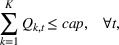
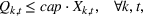
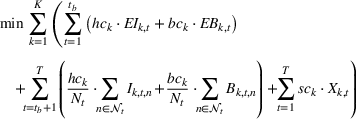
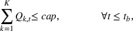
Consider the rolling‐horizon planning of K products with a horizon of T periods. In each review period, updated forecasts are observed and used to calculate a production plan. Let

${\mathbf{F}}^{\mathbf{s}}\in {\mathbb{R}}^{(K\times T)}$

be the forecast vector obtained at the beginning of period s given by

, where

$F_{k,t}^s$

is the forecast of product k in the t‐th period of the planning horizon as seen in review period s. An initial forecast vector denoted by

${\mathbf{F}}^{\mathbf{1}}$

is available. In each review period, a new forecast is also obtained for the last period in the planning horizon. The demand observed at the end of period s is denoted by

$D_k^s$

. After the demand has been observed, the forecast is no longer updated.

Additive MMFE

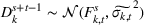
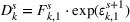
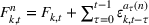
The additive MMFE describes the evolution of the forecast vector by the relation

$${\mathbf{F}}_{\mathbf{post}}^{\mathbf{s}}={\mathbf{F}}^{\mathbf{s}}+{\mathit{\epsilon }}^{s+1},$$

1

where the forecast update vector

${\epsilon }^{s+1}$

is observed at the beginning of review period

$s+1$

. The postupdate forecast vector

${\mathbf{F}}_{\mathbf{post}}^{\mathbf{s}}=[D_1^s,F_{1,1}^{s+1},F_{1,2}^{s+1},\cdots ,F_{1,T-1}^{s+1},\cdots ,D_K^s,F_{K,1}^{s+1},\cdots ,F_{K,T-1}^{s+1}]{}^{⊺}$

contains both the demand

$D_k^s$

observed at the end of period s for all products k and the updated forecasts

$F_{k,t}^{s+1}$

of all products over the horizon. In period

$s+1$

, the planning horizon is rolled forward by one period. The forecast vector

${\mathbf{F}}^{\mathbf{s}+\mathbf{1}}$

is then composed of the updated forecasts in

${\mathbf{F}}_{\mathbf{post}}^{\mathbf{s}}$

and the initial forecasts

$F_{k,T}^{s+1}$

of all products k in the T‐th period of the planning horizon.

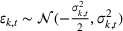
The forecast update vector follows a multivariate normal distribution

${\epsilon }^s\sim \mathcal{MN}(\mathbf{0},\mathrm{\Sigma })$

. The covariance matrix

$\mathrm{\Sigma }\in {\mathbb{R}}^{(K\times T,K\times T)}$

can be expressed as

2

where

${\sigma }_k^t$

is the standard deviation of the t‐th period of the forecast updating process for product k, and

${\rho }_{k_1,k_2}^{t_1,t_2}$

is the correlation between the forecast update of product k ₁ at time t ₁ and product k ₂ at time t ₂. The covariance matrix describes the uncertainty of the forecast updating process over the horizon and the correlation between the forecast updates of different products and time periods.

Demand distribution

The demand follows the same updating process as the forecast and is given by

$D_k^s=F_{k,1}^s+{\epsilon }_{k,1}^{s+1}$

. In any review period s, the demand for the t‐th period in the planning horizon is subject to t forecast updates. As such, the demand in period

$s+t-1$

as seen from period s follows the relation

$$D_k^{s+t-1}=F_{k,t}^s+\sum _{\tau =1}^t{\epsilon }_{k,t-\tau +1}^{s+\tau }.$$

3

Since the forecast update vectors ε are independent and normally distributed, the demand in period

$s+t-1$

follows a normal distribution

$D_k^{s+t-1}\sim \mathcal{N}(F_{k,t}^s,{\stackrel{\sim }{{\sigma }_{k,t}}}^2)$

, where

${\stackrel{\sim }{{\sigma }_{k,t}}}^2={\sum }_{\tau =1}^t{({\sigma }_k^{\tau })}^2$

is the residual uncertainty of the t‐th period in the planning horizon. The residual uncertainty depends only on how far the demand period is in the planning horizon and is a direct measure of the forecast accuracy over the horizon. The demand and forecast revision process are illustrated in Figure 1 for three review periods.

FIGURE 1

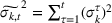
Demand and forecast observed at three successive review periods

Demand covariance

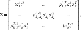
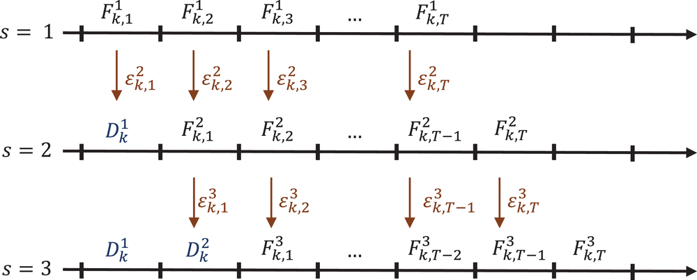
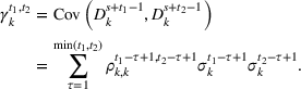
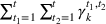
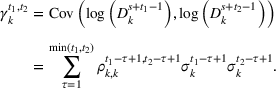
Although the forecast update vectors are observed independently in each review period, the update of different products and time periods described in Equation (1) can be correlated. It follows that the demand distributions of a product in different periods of the planning horizon may be correlated. In review period s, the covariance between the demands of product k in periods t ₁ and t ₂ of the planning horizon is given by

4

The demand correlation depends only on how many forecast update vectors are observed in which the two periods are both in the planning horizon. The covariance between demand observations in different periods is necessary to determine the distribution underlying the cumulative demand.

Cumulative demand distribution

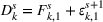
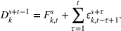
The cumulative demand of product k in period t of the planning horizon at review period s,

$C{D}_{k,t}^s={\sum }_{\tau =1}^t{D}_k^{s+\tau -1}$

, is uncertain since demand is uncertain over the planning horizon. As a sum of correlated, normally distributed random variables, the cumulative demand

$C{D}_{k,t}^s$

follows a normal distribution with mean

${\sum }_{\tau =1}^t{F}_{k,\tau }^s$

and variance

${\sum }_{t_1=1}^t{\sum }_{t_2=1}^t{\gamma }_k^{t_1,t_2}$

.

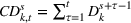
The variance of the cumulative demand depends only on the covariance of the demand distributions of the same product. The variance of the cumulative demand increases linearly with the forecast update correlation between two time periods. The cumulative demand distribution describes the demand uncertainty over the planning horizon. Determining the cumulative demand distributions allows the stochastic lot‐sizing problem to be solved with the formulation introduced in Section 4.

Multiplicative MMFE

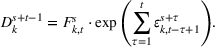
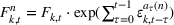
In the multiplicative MMFE, the forecast evolution process follows the relation

$$F_{k,t}^s=F_{k,t+1}^{s-1}·\exp ({\epsilon }_{k,t+1}^s),$$

5

where the forecast update vector

${\epsilon }^s$

follows a multivariate normal distribution

${\epsilon }^s\sim \mathcal{MN}(\mu ,\mathrm{\Sigma })$

and each marginal distribution is given by

${\epsilon }_{k,t}\sim \mathcal{N}(-\frac{{\sigma }_{k,t}^2}{2},{\sigma }_{k,t}^2)$

. The forecast updating process is unbiased, as for the additive model. However, there is a key difference between the two models: In the additive model, forecast uncertainty depends only on the variance of the forecast update distribution, whereas in the multiplicative MMFE, the uncertainty associated with a forecast update is relative to the forecast value. Further, since the multiplicative MMFE is based on a log‐normal distribution, the forecast evolution distribution has a heavier tail than the normal distribution underlying the additive MMFE.

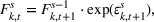
The variance of the forecast updating process depends both on the forecast update covariance matrix Σ and on the forecast vector

${\mathbf{F}}^{\mathbf{s}}$

. Because of these properties, the multiplicative MMFE has been described as more relevant in practice since forecasts tend to be reviewed in a relative manner. The multiplicative model can also be suitable when demand has significant fluctuations over time. In fact, applying a log‐transformation is a well‐known technique to achieve homogeneous variance when data are heteroscedastic such as time‐series forecasting with nonstationary data. Yet, there remain many open questions on how to apply the multiplicative model using available forecast and demand data. In the numerical study in Section 5, we detail the estimation process of the multiplicative model from data and assess its performance in rolling‐horizon planning.

Demand distribution

The demand of product k in each review period s follows the same relation as the forecast update so that

$D_k^s=F_{k,1}^s·\exp ({\epsilon }_{k,1}^{s+1})$

. From this relation and Equation (5), the demand in period

$s+t-1$

as seen from review period s is given by

$$D_k^{s+t-1}=F_{k,t}^s·\exp \left(\sum _{\tau =1}^t{\epsilon }_{k,t-\tau +1}^{s+\tau }\right).$$

6

The demand in period

$s+t-1$

follows a log‐normal distribution,

$\log (D_k^{s+t-1})\sim \mathcal{N}(\log (F_{k,t}^s)-\frac{{\stackrel{\sim }{{\sigma }_{k,t}}}^2}{2},{\stackrel{\sim }{{\sigma }_{k,t}}}^2)$

, where

${\stackrel{\sim }{{\sigma }_{k,t}}}^2={\sum }_{\tau =1}^t{({\sigma }_k^{\tau })}^2$

is the residual uncertainty of the t‐ahead period. The residual uncertainty in the log domain is independent of the review period, as for the additive model. However, demand variance depends on both the forecast update variance and the value of the forecast.

Demand covariance

The demands of product k in periods t ₁ and t ₂ of the planning horizon in review period s are correlated with covariance

7

The demand covariance can be deduced similarly as for the additive case by analyzing the covariance of the forecast evolution process in the log domain. The covariance of the demand periods is used to estimate the parameters of the distribution underlying the cumulative demand.

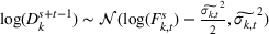
Cumulative demand distribution

Contrary to the additive case, there is no closed‐form expression for the cumulative demand since it is the sum of correlated log‐normal distributions. However, it has been observed that the sum of log‐normal distributions can be well approximated by a log‐normal distribution. To estimate the cumulative demand distributions with multiplicative MMFE, we follow the approach of Norouzi and Uzsoy (2014) and apply the Fenton–Wilkinson approximation (FWA). The method is attractive because of its computational simplicity and overall high approximation quality over a wide range of parameters. The approximation is based on matching the first two moments of the approximating log‐normal distribution with the moments of the sum of the correlated log‐normal distributions (Abu‐Dayya & Beaulieu, 1994).

Following the moment‐matching approximation, the cumulative demand

$C{D}_{k,t}$

approximately follows a log‐normal distribution,

$\log (C{D}_{k,t})\sim \mathcal{N}(m_{k,t},v_{k,t})$

, with parameters

$m_{k,t}=2\log (y_1)-\frac{1}{2}\log (y_2)$

and

$v_{k,t}=\log (y_2)-2\log (y_1)$

, where

$y_1={\sum }_{\tau =1}^t{F}_{k,\tau }$

and

8

This approximate cumulative demand distribution is used in Section 4 to solve the stochastic lot‐sizing problem.

Influence of forecast update correlation on the cumulative demand variance

The variance of the cumulative demand has been shown to depend linearly on the forecast update correlation for the additive model. In the multiplicative model, although the relation between the forecast update correlation and the cumulative demand variance appears exponential, it is approximately linear over the relevant domain. Proposition 1

Under multiplicative MMFE, the variance of the cumulative demand of product k in period t,

$\text{Var}(C{D}_{k,t})$

, is approximately linear in the forecast update correlation

${\rho }_{k,k}^{t_1,t_2}$

for

$t_1,t_2\le t$

with slope given by

$$\frac{\partial \text{Var}(C{D}_{k,t})}{\partial {\rho }_{k,k}^{t_1,t_2}}\approx 2{\sigma }_k^{t_1}{\sigma }_k^{t_2}\exp \left({\beta }_i\right)\sum _{i=1}^{t-t_2+1}{F}_{k,t_1+i-1}{F}_{k,t_2+i-1},$$

9

where

${\beta }_i={\sum }_{\tau =1;\tau \ne i}^{t_1+i-1}{\rho }_{k,k}^{t_1+i-\tau ,t_2+i-\tau }{\sigma }_k^{t_1+i-\tau }{\sigma }_k^{t_2+i-\tau }$

.

Proposition 1 implies that ignoring the correlation between demand periods can lead to under‐ (resp. over‐) estimation of the cumulative demand variance if the correlation is positive (resp. negative). The proof is provided in Supporting Information EC.1. The effect of the correlation coefficient is proportional not only to the variance but also to the forecast values. Thus, ignoring correlation has a greater impact for large forecasts. Moreover, Proposition 1 suggests that the multiplicative model is more sensitive to estimation errors of correlation parameters than the additive model when forecasts are large.

We analyze the evolution of the variance of the cumulative demand distribution with the forecast update correlation and compare the additive and multiplicative MMFE. We consider a single product planned over a horizon of

$T=2$

periods and investigate the effect of forecast update correlation on the cumulative demand

$C{D}^2$

. The forecast updating process is defined with standard deviation

${\sigma }^1={\sigma }^2=20$

for the additive model and

${\sigma }^1={\sigma }^2=0.2$

for the multiplicative model. The initial forecast in periods 1 and 2 are set equal

$F^1=F^2$

and chosen within the set

$\{50,100,150\}$

. The effect of time correlation on the variance of the cumulative demand in period 2 is shown in Figure 2 for the additive and multiplicative models. The figure highlights the linear relationship between the forecast update correlation and the variance of the cumulative demand for both the additive and multiplicative cases. It further illustrates the impact of the forecast value on the variance of the cumulative demand for the multiplicative model.

FIGURE 2

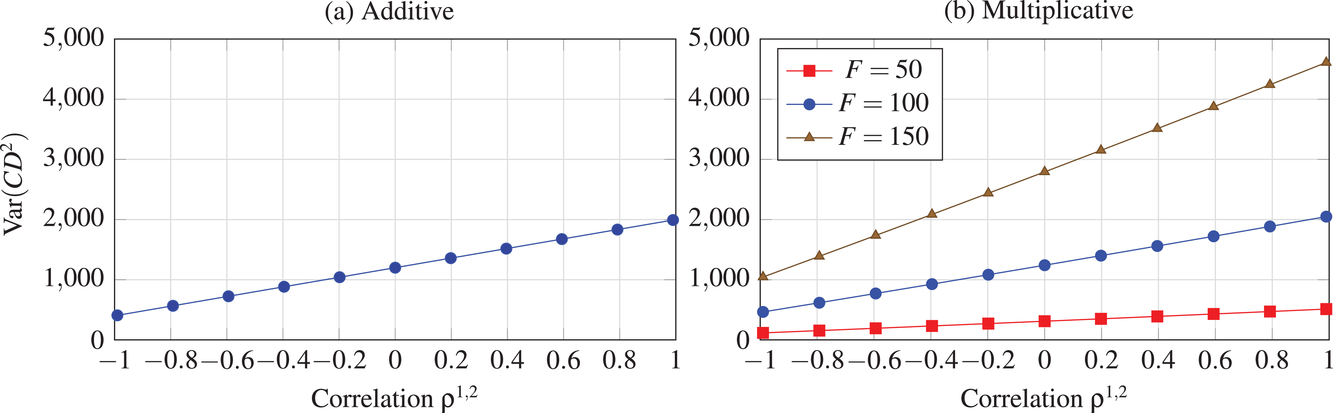
Evolution of variance with correlation coefficient for the (a) additive and (b) multiplicative MMFE

Summary

In this section, the multivariate forecast evolution process has been introduced for additive and multiplicative MMFE. The parameters of the resulting demand and cumulative demand distributions have been obtained. The cumulative demand distributions can be determined exactly for the additive model and approximately for the multiplicative model. Finally, we have analyzed the dependency of the cumulative demand variance on the forecast update correlation coefficient. In the next section, we derive efficient formulations for the stochastic lot‐sizing problem based on the cumulative demand distributions estimated from the MMFE.

INTEGRATING FORECAST EVOLUTION IN STOCHASTIC LOT SIZING

We integrate the additive and multiplicative MMFE in lot‐sizing problems through the cumulative demand distributions derived in the previous section. We introduce the PLA formulation that can be solved efficiently and extend the model with scenario‐based production recourse. The extended model combines the strengths of PLA and scenario methods, providing fast computations and flexible decisions.

Problem setting

In each review period, the planner determines the production quantity

$Q_{k,t}$

for all K products over the planning horizon of T periods. The products share the same equipment with limited capacity

$cap$

in each period. The planner aims to satisfy the uncertain demand while minimizing costs. The operational costs include inventory costs

$h{c}_k$

incurred at the end of each period and setup costs

$s{c}_k$

incurred each time a new product is set up. Unsatisfied demand is backordered and penalized with per‐unit cost

$b{c}_k$

. The initial inventory is denoted by

$i{n}_k^0$

and can be positive or negative depending on whether there is on‐hand inventory or backlog. As demand is uncertain, the inventory

$I_{k,t}$

and backlog

$B_{k,t}$

at the end of each period are random variables. Since they depend on the production quantity, determining their expected value would require nonlinear constraints and lead to intractable formulations.

Linearization of inventory and backlog functions

To obtain tractable formulations, the PLA method has been developed. It evaluates the first‐order loss function at a selected number of breakpoints and determines the slope of the expected inventory and backlog between these breakpoints (Helber et al., 2013). Rossi et al. (2014) provide analytical bounds on the approximation error of PLA when the uncertain variable follows a normal distribution, which applies under additive MMFE. They show that the approximation error is small with only a few linearization points.

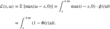
The first‐order loss function of a real variable x and random variable ω with p.d.f. ϕ and c.d.f. Φ is defined as

10

Let

$\mathbf{u}=(u_{k,t,l})$

be the set of

$L+1$

breakpoints determined independently for each product and time period. The first breakpoint is set to

$u_{k,t,0}=i{n}_k^0$

, which can be either positive or negative, and the last breakpoint is set to the highest inventory position attainable at the end of period t with full capacity utilization as

$u_{k,t,L}=i{n}_k^0+cap·t$

. The remaining breakpoints are set uniformly between these two bounds. For each segment, the slope of the expected inventory and backlog can be determined as

11

12

where

$C{D}_{k,t}$

is the cumulative demand distribution of product k in period t. When demand forecasts evolve according to the MMFE, the cumulative demand distributions are updated over the planning horizon in each review period. Hence, the linearization procedure should also be conducted in each period.

Section 3 showed that the cumulative demand follows a normal and log‐normal distribution for additive and multiplication MMFE, respectively. Calculating the slopes of the L segments of the expected inventory and backlog requires evaluating the first‐order loss function

$K·T·(L+1)$

times in each review period. This evaluation is computationally cheap for a normal distribution since the first‐order loss function of a normal variable can be expressed as a function of the first‐order loss function of a standard normal (Rossi et al., 2014), and can thus be calculated offline. The calculation is more expensive for a log‐normal variable since it requires evaluating many integrals as in Equation (10). Note also that the domain of the c.d.f. of a log‐normal variable needs to be extended for negative values since the initial inventory in each period may be negative. The PLA method can be linked back to separable programming, a general framework to solve nonlinear problems using PLAs. Early approaches to solve the resulting model included an adaptation of the simplex algorithm (Bazaraa et al., 2006, section 11.3). We leave for future research to investigate how the special structure of PLA‐based MILP could be exploited as a subclass of separable programming to further improve solution times.

The PLA of two demand distributions following a normal and log‐normal with equal mean and variance is shown in Figure 3. For the chosen parameter values, the functions for both distributions are very similar. The figure shows that the expected inventory and backlog functions can be already well approximated with only

$L=6$

segments for both distributions.

FIGURE 3

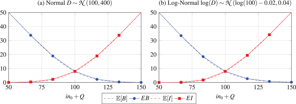
PLA of expected inventory and backlog for demand following (a) a normal distribution and (b) a log‐normal distribution

In practice, the feasible domain of the production variable

$Q\in [0,cap]$

can be large, especially when many products share the same production resource. The inventory and backlog functions are nonlinear only on a restricted part of this domain, as is also illustrated in Figure 3. In principle, techniques could be used to reduce the number of required breakpoints, and thus the calculation times (see, e.g., De Smet et al., 2020). Such approaches would require a search procedure for optimizing the placement of breakpoints. However, in our rolling‐horizon problem, the nonlinear part may change for each planning period and the placement of breakpoints needs to be adapted accordingly. The benefit of reduced calculation times for the MILP is therefore reduced by the search time for the breakpoints. Hence, we use a large number of fixed, equidistant breakpoints in our numerical study to ensure that the nonlinear domain is always well covered.

Stochastic lot sizing without recourse

The PLA formulation of the stochastic lot‐sizing problem approximates the expected inventory and backlog with variables

$E{I}_{k,t}$

and

$E{B}_{k,t}$

, respectively. The key difference in our approach is that the cumulative demand distributions and their linearization are dynamically updated in each review period, following the results presented in Section 3. Additionally, we also adapt the formulation of van Pelt and Fransoo (2018) to account for penalty cost for backlogs. The formulation requires the introduction of auxiliary variables

$w_{k,t,l}$

to measure the cumulative production from period 1 to t associated with segment l and binary auxiliary variables

${\lambda }_{k,t,l}$

to ensure that the L segments are used consecutively. The model is formulated as the following mixed‐integer linear program:

13a

13b

13c

13d

13e

13f

13g

13h

13i

13j

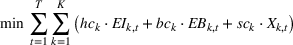
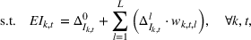
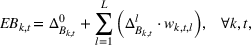
The objective function in (13a) minimizes the expected costs of inventory, backlog, and setup for all products over the horizon. Constraints (13b) and (13c) approximate the expected inventory and backlog using the slopes of the first‐order loss function previously determined. Constraint (13d) determines the production volume from the cumulative production over the linearization segments. Constraints (13e) and (13f) ensure that the linearization segments are used in increasing order through the auxiliary variable

${\lambda }_{k,t,l}$

. These constraints and auxiliary variables are required since the expected backlog function is not convex in the production quantity over the prediction horizon (van Pelt & Fransoo, 2018). Constraint (13g) ensures that the production over all products is limited by the available capacity in each period. Constraint (13h) states that production of a product can occur only if a setup operation is conducted. Constraints (13i) and (13j) describe the domain of positive and binary variables, respectively.

Extended lot‐sizing formulation with production recourse

The stochastic lot‐sizing formulation in (13) provides significant computational improvements compared to traditional scenario‐based stochastic formulations. However, it ignores that the planner has the opportunity to react to forecast updates in each review period. More precisely, Problem (13) defines all production decisions as first‐stage variables, which can lead to overly conservative decisions. Scenario trees can model multistage stochastic processes with recourse decisions. However, they require notoriously long computation times that grow exponentially with the size of the problem instance and scenario tree. We combine PLA and scenario‐based formulations in a single model to allow fast computations and flexible decisions. To reflect the flexibility of this strategy in the planning model while maintaining a reasonable computational effort, we introduce recourse decisions on production variables but not on setup variables. Partial recourse structures can be traced back to Escudero et al. (1993), and are also closely linked to the static–dynamic strategy of Bookbinder and Tan (1988) that implements flexible production decisions with fixed setup decisions. Our numerical studies show that this partial recourse structure improves planning flexibility with only a moderate increase in solution times. In this section, we describe the integration of PLA and scenario‐based recourse decisions, build multistage scenario trees from the MMFE models, and formulate the extended model.

Combining PLA and scenario‐based recourse

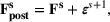
In a multistage stochastic optimization approach, our extended model connects first‐stage decisions for early periods obtained through PLA with recourse decisions for later periods obtained from demand scenarios. For early periods, PLA provides an accurate approximation of the expected inventory and backlog. In parallel, a multistage scenario tree is created to describe the demand and forecast uncertainty over the planning horizon. Applying the first‐stage production decisions from PLA, different inventory positions are reached in the scenario tree. In later periods, the multistage scenario tree allows recourse decisions to react to the different positions created by the first‐stage decisions. Because of the added flexibility, the model can take less conservative first‐stage decisions in the short‐term horizon. Formally, we define

$t_b\in \{1,\cdots T\}$

such that PLA is applied from period 1 to

$t_b$

and scenario recourse is applied from period

$t_b+1$

to T. Clearly,

$t_b=1$

and

$t_b=T$

reduce the approach to a multistage scenario‐based lot‐sizing formulation and the PLA model in (13), respectively.

The scenario‐based extension of the PLA model can be seen as an approximation of the optimal production policy that would be obtained if the corresponding dynamic programming model were solved. The scenario part of the model acts as a look‐ahead approximation of the optimal policy (Powell, 2016). There are two main advantages for applying PLA for early periods and scenario trees with recourse for later periods. First, it is well known that the approximation quality of scenario‐based formulations increases with the number of scenarios. Multistage scenario trees grow exponentially over the planning horizon because of their branching structure. As such, only few scenarios describe the uncertainty in the short‐term horizon and the approximation error is high specifically for the immediate periods that are most important for planners. By using the PLA formulation over the short‐term horizon, we ensure low approximation error in the periods with few scenarios while still benefiting from the flexibility of multistage models over the long‐term horizon. Second, the introduction of recourse production decisions leads to a lack of a reference plan since production decisions are conditioned on the discrete scenarios. By using only first‐stage decisions over the short‐term horizon, our method ensures the availability of a reference plan, which is often indispensable in industry. The trade‐off between flexibility and availability of a reference plan is adjusted through choosing parameter

$t_b$

.

Let

${\mathcal{N}}_t$

be the set of demand scenarios in period t. Over the planning horizon, there are

$[N_1,N_2,\cdots ,N_T]$

scenarios where

$N_t$

is the number of demand scenarios in period t. The combination of PLA and scenario‐based recourse in our approach is illustrated in Figure 4. Here, the multistage scenario tree is generated with a branching factor of 2 over a planning horizon of

$T=6$

periods with

$t_b=3$

. Thus, there are [2, 4, 8, 16, 32, 64] demand scenarios, [1, 2, 4, 8, 16, 32, 64] inventory positions, and [1, 1, 1, 8, 16, 32] production decisions over the horizon.

FIGURE 4

Demand observations, production decisions, and inventory trajectories over

$T=6$

periods with

$t_b=3$

Generating scenario trees from forecast evolution

The demand scenario tree is generated from the MMFE from period 1 to T by updating the initial forecast

${\mathbf{F}}^{\mathbf{s}}$

with forecast update vectors sampled in each node. The forecast update vectors are drawn from the multivariate forecast evolution distribution. The forecast of product k in period t of the horizon in scenario node n can be expressed as

$F_{k,t}^n=F_{k,t}+{\sum }_{\tau =0}^{t-1}{\epsilon }_{k,t-\tau }^{a_{\tau }(n)}$

for the additive MMFE and

$F_{k,t}^n=F_{k,t}·\exp ({\sum }_{\tau =0}^{t-1}{\epsilon }_{k,t-\tau }^{a_{\tau }(n)})$

for the multiplicative MMFE where

${\epsilon }^{a_{\tau }(n)}$

is the forecast update vector obtained at node

$a_{\tau }(n)$

, the τ‐th ancestor node of node n with

$a_0(n)=n$

.

Many techniques have been developed to generate scenario trees from probability distributions. In this paper, we use Latin Hypercube because of the high variance reduction observed empirically (Linderoth et al., 2006) and the simplicity of its implementation. To sample the high‐dimensional, correlated forecast update vectors in each node, we apply the Latin hypercube with multivariate uniformity (LHMU) method developed by Deutsch and Deutsch (2012) designed to reduce sampling variability for high‐dimensional multivariate random variables. Other techniques such as optimal quantization or moment matching may also be applied although they often increase computation times (Heitsch & Römisch, 2009; Löhndorf, 2016).

Extended lot‐sizing formulation

The extended stochastic lot‐sizing formulation with PLA and scenario‐based recourse is given by:

14a

14b

14c

14d

14e

14f

14g

14h

14i

14j

14k

14l

14m

14n

14o

The objective function in (14a) minimizes the PLA expected inventory and backlog costs over the first

$t_b$

periods and the sample average inventory and backlog costs over the remaining

$T-t_b+1$

periods. Constraints (14b) to (14h) are adapted from the PLA model to the first

$t_b$

periods. Constraints (14i) and (14j) describe the discrete inventory positions through the planning horizon with first‐stage and recourse production decisions, respectively. The operator

$a_1(n)$

returns the index of the direct ancestor of node n in the multistage scenario tree. This formulation implicitly enforces the so‐called nonanticipativity constraints, ensuring that decisions in a time period cannot use information obtained in later periods, as is also illustrated in Figure 4. Note that the discrete inventory and backlog determined in Constraint (14i) are not used in the objective function. They determine sample inventory positions at the end of periods

$t_b$

resulting from the first‐stage decisions. Constraints (14m) and (14n) specify the domain of the continuous first‐stage and recourse variables. Constraint (14o) specifies the binary variables.

Summary

This section has introduced a general stochastic lot‐sizing approach apt for use in rolling‐horizon planning. The forecast evolution models described in Section 3 are integrated in the lot‐sizing problem through the cumulative demand and forecast evolution distributions. We have shown that both additive and multiplicative MMFE models can be readily included in lot‐sizing problems through PLA. The model was extended to allow for production recourse for later periods through a discrete scenario tree. We have shown how the scenario tree can be constructed by sampling the multivariate distribution describing the forecast evolution process.

NUMERICAL STUDY

The numerical study investigates the use of forecast evolution models in stochastic lot sizing from model estimation to application. Our assessment is based on extensive rolling‐horizon simulations. We answer the following questions:

How can MMFE model parameters be estimated from real data?

What is the value of forecast evolution models in practice?

What are the strengths and weaknesses of the additive and multiplicative MMFE?

What is the value of recourse provided by our multistage formulation?

What factors influence the value of recourse?

The numerical study is composed of three main parts. First, we solve the real‐world case study of a global company in the process industry. A large data set of forecast and demand history is used to estimate the MMFE models and assess their performance. Simulations are run in an out‐of‐sample setting in which the forecast evolution process is unknown and can only be estimated from historical data. Second, we use synthetic data to analyze in detail the effect of not knowing the distribution underlying the forecast evolution. We specify the forecast evolution distributions for the additive and multiplicative models and simulate them in a rolling‐horizon fashion. Since the forecast evolution process is fully known in these experiments, we are able to evaluate the value of using the additive model when the actual forecast evolution follows a multiplicative model and conversely. Further, we quantify the value of recourse for the MMFE model with a known forecast evolution process. Sensitivity analyses are set up to identify parameters that drive the performance of forecast evolution models including demand fluctuation, capacity, and the variance of MMFE models. In a third part, we summarize our findings and provide general recommendations on the use of MMFE models.

The numerical study is implemented in Julia (Bezanson et al., 2017). The optimization problems are modeled in JuMP (Dunning et al., 2017) and solved with Gurobi 9.0. The relative objective gap of the solver is set to 1% for all models. The calculations are run on an Intel(R) Core(TM) i7‐4810MQ processor at 2.80 GHz using 16GB of RAM. The code used to produce the results and figures based on synthetic data is made publicly available on the online repository (https://github.com/alexforel/DynMMFE).

Real‐world case study

We apply our approach to the real‐world case study of a large company manufacturing chemical products used in agriculture. Demand follows the growth cycle of crops and exhibits strong seasonality and high uncertainty. In each planning period, demand forecasts are obtained through a sales and operations planning (S&OP) process that combines expert evaluations and automated calculations. The demand forecasts are determined for all products of a large product portfolio. We focus on the tactical planning level with a long production horizon. At this level, planning decisions are made on an aggregated product‐family level. The families have been designed such that cleaning operations are required each time a new family is set up. Thus, our analysis covers

$K=6$

product families (henceforth referred to as products) that share the same production resource. Together with our industry partner, we gathered the history of forecasts and demand at a monthly granularity over 4 years. We then aggregate the forecast and demand data on the family level. Data and costs are reported in unit of measurement (u.o.m.) and cost unit (c.u.), respectively, for confidentiality reasons.

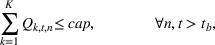
The historical demand and its clear yearly seasonality are shown in Figure 5. The planning horizon is set to

$T=8$

to capture the majority of the season while keeping computation times low. The inventory costs are determined together with our industry partner and range between 0.04 and 0.1 c.u per u.o.m. per month across the products. The backlog costs are set to

$b_c=15·h_c$

and the setup costs to

$s_c=15$

 c.u. The initial inventory is set to zero. The monthly production capacity is given as

$cap=4934$

u.o.m. per month. The PLA‐based lot‐sizing models introduced in Section 4 are implemented with

$L=60$

breakpoints. The extended model uses a scenario tree with [3, 6, 6, 12, 12, 24, 24, 48] nodes over the planning horizon sampled with LHMU. The extended model is parameterized with

$t_b=4$

so that the first half of the planning horizon uses first‐stage decision variables and the second half uses production recourse.

FIGURE 5

Four‐year demand history for the six families of chemical products investigated in the industry case

Estimating MMFE models from historical data

Simulations are run in an out‐of‐sample fashion to provide unbiased estimates of model performance and to assess the ability of MMFE models to generalize from past observations. In each review period, only past observations of the forecast evolution process are used to estimate the MMFE parameters. The simulation starts in period 25 so that half the data set is available to estimate the MMFE parameters in the first simulation period, and half the data set is used for the rolling‐horizon evaluation. In each review period, model parameters are re‐estimated from the history of forecast updates in an online fashion.

While the empirical mean and covariance matrix of the additive MMFE can be estimated easily, the occurrence of zero values for the forecast and demand complicates the estimation for the multiplicative model. Because the multiplicative model assumes that demand and forecasts are always positive, all forecast and demand vectors in which at least one value is zero are removed from the data set. In total, this amounts to around 50% of the data set. We then determine the parameters of the log‐normal distribution as the empirical mean and covariance of the log of the forecast updates. Thus, we find the maximum likelihood estimators of the forecast update distribution parameters for both additive and multiplicative MMFE. To conform to the assumption of an unbiased forecast underlying the MMFE models, we additionally correct the sample bias. The estimated covariance matrices exhibit complex correlation structures. Interestingly, the additive MMFE exhibits strong positive correlation for the first three products over the horizon, while the multiplicative MMFE has high positive time correlations for the two last products. The difference between the correlation parameters of the two MMFE models can be explained by the censoring of forecast updates with a value of zero in the multiplicative model. Such updates occur more frequently in the low season.

After estimating the distribution parameters, a practitioner might be interested in evaluating the goodness‐of‐fit of the forecast update samples to the distributional assumptions of the additive and multiplicative models. Intuitively, one would think that the goodness‐of‐fit provides a first measure of the expected performance of the MMFE models. A Shapiro–Wilk test is performed over the whole data set on each marginal distribution of the additive and multiplicative models. The statistical tests reject the hypothesis that the forecast updates are normally distributed with strong confidence for all products and all time periods for the additive model. The results are more nuanced for the multiplicative model as the distribution hypothesis cannot always be rejected with strong confidence. This first analysis suggests that the multiplicative model, having a better fit to the data, is likely to provide good results whereas the additive model should perform poorly. The detailed results of the goodness‐of‐fit tests are provided in Supporting Information EC.2.

Out‐of‐sample simulation results

In our numerical simulations, we notice that the presence of outliers can significantly impact model performance. In this context, outliers are understood as large forecast updates (positive or negative), which disrupt the estimation of the MMFE parameters. To remove outliers, forecast updates belonging to the upper and lower α quantiles are ignored when estimating MMFE parameters in each planning period. This method is known as trimming and has been used in diverse settings such as robust regression (Bertsimas et al., 2017). Outlier data are removed independently for each product and time period in the planning horizon so that the marginal distributions of trimmed MMFE models are assumed independent. We choose the value

$\alpha =10\%$

for the trimming factor as a good compromise between generalization and robustness to outliers.

Currently, our company partner implements a deterministic planning in a rolling‐horizon fashion. We introduce a deterministic model that uses the available point‐estimate forecasts directly and ignores demand uncertainty to benchmark this practice. Due to the seasonality of demand, only few observations of the demand process are available. As such, we do not implement a stochastic benchmark based only on the demand data. The simulation results over the 24 periods are presented in Table 1. The additive MMFE model with PLA reduces costs by 11% compared to the deterministic model, thanks to relevant safety stock that increase inventory costs but provide a significant reduction in backlog and setup costs. The extended additive model with production recourse further reduces costs by 3% through less conservative inventory decisions. The multiplicative model performs poorly over the simulation as it builds large inventory reserves. These results are particularly noteworthy for two reasons. First, they contradict the goodness‐of‐fit analysis that suggested that the additive MMFE would not be an appropriate model. Second, they contradict the consensus that multiplicative MMFE is preferable when demand fluctuates over time.

TABLE 1

Results of out‐of‐sample case study: Realized costs (in c.u)

Model	Total cost (rel.)		Inventory cost (rel.)		Backlog cost (rel.)		Setup cost (rel.)
Deterministic	3513	(100%)	796	(100%)	1442	(100%)	1275	(100%)
Additive PLA	3116	(89%)	1293	(162%)	803	(56%)	1020	(80%)
Extended Add. PLA	3015	(86%)	1112	(140%)	868	(60%)	1035	(81%)
Multiplicative PLA	3612	(103%)	2424	(304%)	288	(20%)	900	(71%)
Extended Mult. PLA	3560	(101%)	2431	(305%)	259	(18%)	870	(68%)

To explain the poor performance of the multiplicative model, we conduct a sensitivity analysis of the trimming factor α. The trimming factor is varied between 0% and 25%. Because zero forecast values are removed when estimating the parameters of the multiplicative model, only few samples are available as the trimming factor increases. It is not possible to investigate trimming factors greater than

$\alpha =25$

since only one sample is then available and the parameters of the multiplicative MMFE cannot be estimated. The results of the sensitivity analysis are shown in Figure 6. The sensitivity of the multiplicative model to the trimming factor is striking. In fact, the multiplicative model performs best when it uses as few samples as possible, thereby artificially reducing the overconservativeness of the model. On the other hand, the additive model performs robustly and consistently outperforms the deterministic benchmark.

FIGURE 6

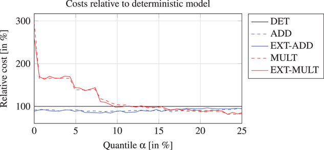
Sensitivity analysis of model performance to outlier trimming

Several factors explain the worse performance of the multiplicative model. First, the censoring of forecast update with a value of zero leads to an overestimation of demand variance in the multiplicative model. Second, the multiplicative model has a higher sensitivity to estimation error as discussed in the interpretation of Proposition 1. Since uncertainty is relative to the forecast itself, an estimation error on variance parameters can have a large effect on the peak of the seasonal demand. This can be further amplified by the presence of outliers in the data, as is shown in the trimming analysis. Another explanation is that the multiplicative model fails to generalize to settings in which the true forecast evolution process does not follow a multiplicative MMFE. Goodness‐of‐fit tests measure how well the historical data follow the distributional assumption of the MMFE models and suggest that the multiplicative MMFE better fits past data. They assess the normality of the log‐updates but do not provide any guarantee on the performance of the MMFE‐based model in rolling‐horizon planning.

Minimizing estimation errors and minimizing planning costs are two different tasks (Elmachtoub et al., 2020; Elmachtoub & Grigas, 2022). In fact, prediction models with low estimation error may yield higher costs than other seemingly less precise models (Ferber et al., 2020). Hence, an explanation of the poor performance of the multiplicative model may be that the estimation error minimized when fitting the model is less closely linked to the planning costs than the estimation error used when fitting the additive model. Adapting the model fitting procedure to take into account planning costs is an interesting but challenging research direction. Differing from the simpler class of problems studied by Elmachtoub and Grigas (2022), our problem is dynamic and implemented in a rolling‐horizon fashion. Further, the uncertain parameters have nonlinear effects on the objective function.

To better understand the shortcomings of the multiplicative model and to identify situations in which it is better to use an additive model, we perform an extensive numerical study with synthetic data in the following section. In particular, we evaluate the cost of model misspeficiation for demand patterns with different dynamics.

Synthetic data

In this section, the forecast evolution process described by the MMFE is simulated on artificial instances. By performing sensitivity analyses of key parameters, we evaluate the performance of MMFE‐based models in a variety of problem settings. In particular, we vary the capacity, uncertainty, and demand patterns. We also aim to provide insights on the use of MMFE‐based models in real‐life situations in which underlying probability distributions are unknown. To this end we employ the additive model when the true forecast evolution process is multiplicative and conversely. Then, we assess our multistage extension and identify drivers that influence the value of recourse enabled by it.

Simulation instances

We consider

$K=2$

products over a prediction horizon of

$T=6$

periods. Each simulation contains

$S=12$

review periods. The inventory holding costs are sampled randomly for the two products as

$h_c\sim \mathcal{U}[1,1.5]$

. The backlog cost is set to

$b_c=10·h_c$

and the setup cost is set to

$s_c=150$

. The initial inventory is set to

$i{n}^0=50$

for each product. The PLA method uses

$L=40$

segments, which ensures a low approximation error. The extended model uses a scenario tree with [3, 6, 12, 24, 48, 48] nodes over the planning horizon sampled with LHMU. We set

$t_b=3$

so that the first half of the planning horizon is modeled with PLA and the second half with scenario recourse.

The capacity in each period is chosen as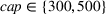

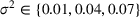
$cap\in \{300,500\}$

to reflect settings with limited and ample capacity. The initial forecast values are generated from three demand patterns with different dynamics. Stationary, random, and seasonal patterns are used as illustrated in Figure 7. The stationary pattern sets the initial forecasts to a constant value

$F=100$

over the simulation length. The random pattern samples each initial forecast from the uniform distribution

$\mathcal{U}[50,150]$

. The seasonal pattern is generated with periodicity

$S/2$

from a sine function, which yield values [16, 93, 145, 159, 129, 65] as initial forecasts over the season length. The three demand patterns have the same average demand over the simulation length but different dynamics, which may impact the additive and multiplicative MMFE models differently. The forecast evolution models are set unbiased and uncorrelated with equal forecast update variance for all products and time periods. Low, medium, and high forecast uncertainty settings are defined with variance

${\sigma }^2\in \{100,400,700\}$

for the additive model and

${\sigma }^2\in \{0.01,0.04,0.07\}$

for the multiplicative model. Thus, the two forecast evolution models have the same variance under the average demand.

FIGURE 7

Mean demand for (a) stationary, (b) random, and (c) seasonal patterns over simulation of eight periods

MMFE models and benchmarks

In practice, the true forecast evolution is unknown. To estimate the value of MMFE‐based lot sizing when using a mismatched forecast evolution model, we run two distinct sets of simulations in which the forecast evolution process follows the assumptions of the additive and multiplicative MMFE. The mismatched model is estimated from a simulation of the true forecast evolution process over 1 million periods. The sampled forecast updates are measured according to the mismatched MMFE model and used to estimate its parameters.

As in the previous real‐world case study, the estimation procedure of the multiplicative model is not straightforward. When the forecast evolution process follows an additive MMFE, demand is normally distributed and demand observations may be zero (or negative, which is corrected to zero in all simulations of additive MMFE). It is also possible that a forecast with value of zero is updated to a positive forecast. These two cases, while frequently occurring in practical settings, are not compatible with the multiplicative MMFE. Thus, when estimating the parameters of the multiplicative MMFE, we remove all sampled forecasts that contain at least one zero value. For the setting with low uncertainty, this amounts to removing 0%, 1%, and 41% of samples for the stationary, random, and seasonal patterns, respectively; 13%, 26%, and 64% for the medium uncertainty setting; and 37%, 50%, and 74% for the high‐uncertainty setting. Clearly, more sample updates are removed from the data set as the demand pattern is more dynamic and as uncertainty increases. The high number of unusable samples is an important shortcoming of multiplicative MMFE since collecting data is an expensive process.

Two benchmarks are introduced: (1) a deterministic model that uses the forecast as a point estimate and ignores uncertainty but observes the updated forecasts in each planning period and (2) a demand‐driven stochastic model that ignores forecasts and their evolution and instead estimates demand distributions from historical data. For the stationary and random patterns, the demand‐driven model estimates a stationary demand distribution. For the seasonal pattern, the demand‐driven model estimates independent distributions for all periods in the season. The model estimates the parameters of normal and log‐normal distributions from simulations of the forecast evolution process over 1 million periods using additive and multiplicative MMFE, respectively. These two models benchmark the planning practices of industry and the traditional stochastic lot‐sizing literature, respectively. The performance of stochastic models is traditionally evaluated by measuring the value of the stochastic solution (VSS), which is based on a static evaluation of the deterministic and stochastic models, and the expected value of perfect information (EVPI), which measures the value of obtaining perfect forecasts (Birge & Louveaux, 2011). By comparing the performance of the stochastic models to the deterministic benchmark implemented in a rolling‐horizon fashion, we extend the VSS to a more realistic setting in which the deterministic benchmark also benefits from updated forecasts. Further, the value of improving the forecasting process is measured by comparing the costs of MMFE‐based models under the different uncertainty settings, providing a richer performance evaluation than the EVPI.

Results

Each rolling‐horizon simulation of the 36 instances is repeated 1000 times. Model performance is measured as the sum of realized inventory, backlog, and setup costs. The results under additive and multiplicative MMFE are presented in Table 2 and Table 3, respectively, as the average of the costs over the 1000 repetitions. The statistical significance of all relative cost differences from the deterministic model is assessed using Student's t‐test. Statistical significance is indicated with the symbol (*) for all relative values for which the associated p‐value is strictly smaller than 5%.

TABLE 2

Simulation results when forecast evolution follows an additive MMFE process

Demand	Uncertainty	$cap$	Det.	DD‐stochastic	Additive PLA (correct model)	Multiplicative PLA (mismatched model)	Extended Add. PLA (correct model)
Stationary	Low	300	4707.9	4711.9  (100.6%*)	4153.6  (88.6%*)	4118.4    (87.9%*)	4135.6  (88.2%*)
		500	4676.2	4695.8  (100.9%*)	4152.0  (89.2%*)	4129.8    (88.7%*)	4131.0  (88.8%*)
	Medium	300	5312.4	5680.1  (108.2%*)	4652.2  (88.6%*)	5147.5    (98.0%*)	4593.8  (87.4%*)
		500	5069.4	5722.9  (114.0%*)	4589.3  (91.3%*)	4974.9    (99.1%*)	4541.4  (90.4%*)
	High	300	5927.2	6326.7  (109.5%*)	4923.7  (85.2%*)	6689.6  (116.2%*)	4878.4  (84.4%*)
		500	5421.0	6265.6  (117.2%*)	4811.5  (89.8%*)	5712.9  (106.8%*)	4770.0  (89.1%*)
Random	Low	300	4581.2	5365.6  (117.8%*)	4020.2  (88.2%*)	4122.6    (90.5%*)	4007.5  (87.9%*)
		500	4515.3	5367.6  (119.5%*)	3986.4  (88.7%*)	4063.5    (90.5%*)	3969.7  (88.3%*)
	Medium	300	5336.4	6093.5  (116.0%*)	4568.2  (86.9%*)	5586.9  (106.4%*)	4501.4  (85.6%*)
		500	5078.3	6009.9  (119.6%*)	4473.4  (89.0%*)	5134.8  (102.2%*)	4418.0  (87.8%*)
	High	300	6077.4	6645.8  (112.7%*)	4914.6  (83.3%*)	7209.2  (123.1%*)	4863.4  (82.4%*)
		500	5525.4	6523.9  (120.1%*)	4749.0  (87.3%*)	5968.2  (109.8%*)	4712.2  (86.6%*)
Seasonal	Low	300	4598.6	4507.7    (99.1%*)	3968.4  (87.1%*)	5785.4  (127.3%*)	3932.9  (86.3%*)
		500	4187.3	4229.0  (101.7%*)	3720.9  (89.4%*)	4589.2  (110.3%*)	3683.8  (88.5%*)
	Medium	300	5713.3	5771.8  (104.4%*)	4575.6  (82.4%*)	8225.2  (148.8%*)	4505.9  (81.0%*)
		500	4957.1	5309.8  (108.5%*)	4222.4  (86.2%*)	5931.2  (121.1%*)	4159.6  (84.8%*)
	High	300	6609.7	6703.3  (107.7%*)	5066.8  (81.0%*)	9573.1  (156.0%*)	4970.3  (78.5%*)
		500	5425.5	5913.5  (111.1%*)	4501.8  (84.4%*)	7911.5  (148.5%*)	4463.4  (83.7%*)
Average			5206.6	5658.0  (108.7%*)	4447.2  (85.4%*)	5826.3  (111.9%*)	4402.1  (84.5%*)

TABLE 3

Simulation results when forecast evolution follows a multiplicative MMFE process

Demand	Uncertainty	$cap$	Det.	DD‐stochastic	Additive PLA (mismatched model)	Multiplicative PLA (correct model)	Extended Mult. PLA (correct model)
Stationary	Low	300	4695.2	4801.1  (102.8%*)	4179.1  (89.5%*)	4151.7  (88.9%*)	4124.0  (88.2%*)
		500	4616.2	4776.1  (104.0%*)	4190.7  (91.2%*)	4149.5  (90.3%*)	4117.3  (89.6%*)
	Medium	300	5452.8	6187.3  (115.4%*)	4852.8  (90.8%*)	4785.2  (89.8%*)	4691.1  (87.7%*)
		500	5059.3	6082.8  (121.3%*)	4713.1  (94.2%*)	4644.4  (92.9%*)	4571.7  (91.3%*)
	High	300	6440.5	7368.2  (118.4%*)	5414.7  (87.6%*)	5469.3  (90.1%*)	5223.9  (84.6%*)
		500	5494.7	7168.7  (132.1%*)	5035.5  (93.3%*)	5049.4  (94.2%*)	4909.8  (91.3%*)
Random	Low	300	4634.3	5566.5  (120.9%*)	4088.5  (88.8%*)	4018.2  (87.3%*)	3999.5  (86.8%*)
		500	4524.1	5528.9  (122.9%*)	4019.0  (89.3%*)	3956.3  (88.0%*)	3925.1  (87.2%*)
	Medium	300	5576.9	6763.9  (124.2%*)	4851.8  (89.4%*)	4771.3  (88.4%*)	4625.9  (85.2%*)
		500	5055.6	6677.1  (133.6%*)	4637.0  (92.9%*)	4534.6  (91.1%*)	4438.6  (89.0%*)
	High	300	6675.1	8012.7  (126.6%*)	5632.6  (89.5%*)	5596.4  (91.3%*)	5350.8  (85.1%*)
		500	5575.4	7657.9  (139.4%*)	5048.3  (92.7%*)	5019.1  (92.9%*)	4856.8  (89.5%*)
Seasonal	Low	300	4806.4	4761.8  (100.8%  )	4171.4  (87.9%*)	4082.0  (86.4%*)	4021.5  (84.9%*)
		500	4276.3	4510.2  (106.4%*)	3856.3  (90.8%*)	3749.0  (88.3%*)	3701.3  (87.2%*)
	Medium	300	6435.3	6623.6  (109.7%*)	5265.7  (85.9%*)	5286.7  (88.7%*)	5054.5  (82.1%*)
		500	5162.3	6125.6  (120.9%*)	4635.4  (91.6%*)	4428.2  (88.1%*)	4331.7  (86.0%*)
	High	300	7762.7	8105.1  (116.3%*)	6169.5  (87.1%*)	6404.2  (95.0%*)	5977.3  (82.4%*)
		500	5835.7	7329.8  (130.3%*)	5102.6  (90.5%*)	5024.9  (90.7%*)	4780.2  (85.5%*)
Average			5448.8	6336.0  (116.3%*)	4770.2  (87.5%*)	4728.9  (86.8%*)	4594.5  (84.3%*)

Our simulation results quantify the value of forecast evolution models compared to both traditional deterministic approaches typical in industry and stochastic models that focus solely on historical demand data and ignore forecast. The costs of the deterministic benchmark are especially high when capacity is tight, uncertainty is high, and demand fluctuates over time. It is also in these settings that the MMFE models with known forecast evolution provide large cost reductions. The stochastic, demand‐driven model increases costs compared to the naive deterministic model for almost all instances. This can be explained by two reasons. First, the model is overly conservative since it accounts for the whole demand uncertainty for all periods in the planning horizon. Second, it is inaccurate because it only aims for the average observed demand and ignores the forecasts. This is especially true for the random demand pattern since, even though demand is stationary, the initial forecast values provide a lot of information on the final demand observations. On the other hand, the additive and multiplicative MMFE models reduce costs by 14% on average compared to the deterministic model when the forecast evolution process is known.

The value of improving the forecasting process to reduce forecast uncertainty can be measured by comparing the costs of the correct MMFE model in different uncertainty settings. For instance, under additive MMFE in the seasonal setting with low capacity, the planner would be willing to pay up to 580 c.u. to reduce the forecast uncertainty from the high uncertainty to medium uncertainty, and up to 500 c.u. to reduce it further to the low uncertainty setting. Interestingly, the value of information appears higher in the simulation settings with low capacity. This result contrasts with previous studies that found that advance information was not useful when utilization is high (Albey et al., 2015; Ziarnetzky et al., 2018, 2020). This difference can be mainly explained by the fact that previous literature uses several approximations such as capacity allocation when determining the safety stocks of the different products. This severely restricts planning flexibility when utilization is high. Flexibility is even more important in our experiments since we consider products with different cost parameters whereas Ziarnetzky et al. (2018) and Albey et al. (2015) consider symmetric products. A detailed analysis of the effect of the simulation parameters and their interactions is given in Supporting Information EC.3.

The cost of model misspecification is high for the multiplicative model. Indeed, Table 2 shows that using a multiplicative forecast evolution model when the true process is additive can significantly increase costs even compared to traditional deterministic planning. On average, the costs of the multiplicative model are 12% larger and more than 50% when demand is seasonal and uncertainty is high as is the case in our industry application. In contrast, the cost of model mis‐specification is low for the additive model. Table 3 shows that when the true process is multiplicative, the additive model yields costs almost as low as the multiplicative model, suggesting that additive MMFE‐based models are robust to errors in modeling the forecast evolution process. These results explain the superiority of the performance additive model for our industry case, in which the true forecast evolution process is unknown.

Value of recourse

The value of recourse is defined as the difference between costs of the stochastic model without recourse and the extended stochastic model combining PLA and scenario‐based recourse, as presented in Table 2 and Table 3. The value of recourse varies over the simulation settings similarly for both MMFE models. It is higher for more complex planning settings: When demand is dynamic, uncertainty is high, and capacity is limited. Overall, recourse is more beneficial under multiplicative MMFE. On average, the value of recourse is around 1.5% and 2.5% across all simulation settings and can reach 2.3% and 6.2% for the additive and multiplicative models, respectively. The detailed statistical analysis of the value of recourse is given in Supporting Information EC.4. It shows that these results are statistically significant at a p‐value smaller than 5%. The distribution of the value of recourse is skewed so that in the majority of cases, observed costs are smaller than the average value. To further investigate the value of recourse in stochastic models and to identify settings in which it is most beneficial, we perform several sensitivity analyses.

Impact of product and time correlation

In Section 3, we have shown that positive (resp. negative) forecast time correlation was equivalent to a higher (resp. lower) cumulative demand variance for both MMFE models. For the extended model with recourse, correlation has an even larger impact since the recourse model can react to correlated forecast updates. We analyze the impact of the correlation structure on the value of recourse on the simulation setting with seasonal demand and

$cap=300$

. The influence of both product and time correlation is investigated. Product correlation is set constant over the horizon as

${\rho }_{1,2}^{t,t}={\rho }_k$

with

${\rho }_k\in \{-0.6,0,0.6\}$

. Time correlation is set between the first and second periods of the horizon for both products as

${\rho }_{k,k}^{1,2}={\rho }_t$

with

${\rho }_t\in \{-0.6,0,0.6\}$

. If both product and time correlation parameters are nonzero, then the first and second periods of the two products are also correlated. In this case, we set

${\rho }_{1,2}^{1,2}={\rho }_k·{\rho }_t$

.

The costs of the extended model with recourse relative to the costs of the model without recourse are presented in Table 4. The statistical significance of the relative cost is assessed with Student's t‐test and is shown with the symbol (*) if the p‐value is below 0.05. The correlation structure has a strong impact on the value of recourse. Negative time correlation yields high value of recourse for both MMFE models, whereas positive time correlation leads to lower values than in the uncorrelated case. Recourse decisions can take advantage of negative time correlation by anticipating that forecast updates will compensate over time. Specifically, a forecast increase for the first period in the horizon might be compensated by a forecast decrease in the second period. Anticipating this effect leads to less conservative decisions. Hence, the largest improvements are observed when time correlation is negative and product correlation is positive. Here, a compensation over time occurs for both products and costs can be reduced by more than 10% compared to the stochastic model without recourse. This analysis shows the importance of including correlation in stochastic planning especially when using recourse models. Further, it confirms the trend that the multiplicative model benefits most from recourse.

TABLE 4

Value of recourse for different correlation structures

	Additive MMFE			Multiplicative MMFE
	${\rho }_k=-0.6$	${\rho }_k=0$	${\rho }_k=0.6$	${\rho }_k=-0.6$	${\rho }_k=0$	${\rho }_k=0.6$
${\rho }_t=-0.6$	97.4 (*)	96.9 (*)	96.8 (*)	92.1 (*)	91.2 (*)	89.2 (*)
${\rho }_t=0$	98.3 (*)	98.5 (*)	99.0 (*)	93.9 (*)	94.6 (*)	93.3 (*)
${\rho }_t=0.6$	98.7 (*)	100.1	100.9 (*)	97.4 (*)	97.1 (*)	95.8 (*)

We also perform extensive sensitivity analyses of the available capacity and scenario structures. The sensitivity analysis of capacity shows that the value of recourse increases monotonously with the available capacity under additive MMFE. The value of recourse is larger under multiplicative MMFE and peaks when capacity is neither too limited nor too large. The sensitivity analysis of the scenario structure shows that scenario trees with an intermediate size, such as the one used throughout this section, are sufficient to benefit from recourse without substantial increase in computation times. Details on both sensitivity analyses are provided in Supporting Information EC.5.

The value of flexibility is also studied in a broader context in Supporting Information EC.6 by comparing the value of recourse to the value of a free‐return policy, which allows to liquidate excess inventory at no cost. The numerical results confirm that flexibility is more valuable under multiplicative MMFE than additive MMFE. Recourse and returns decisions are two flexibility levers that provide large cost reductions under multiplicative MMFE. Recourse decisions are more beneficial when capacity is tight whereas return decisions prove especially valuable when capacity is large.

Summary and recommendations

The numerical study shows that integrating forecast evolution models in stochastic lot sizing can significantly improve planning quality compared to traditional deterministic approaches and stochastic methods based solely on demand data. The additive MMFE model is robust and performs well across all simulation instances: (1) when the forecast evolution process is known, (2) when it is unknown and estimated from mismatched updates, and (3) when it is learned from real‐world historic data. Interestingly, the cost savings provided by stochastic models based on additive MMFE relative to the deterministic benchmark are similar on both the real‐world and the synthetic data. On the other hand, the multiplicative model suffers from several limitations, which have been identified through our extensive numerical studies. First, the multiplicative model is particularly sensitive to model misspecification: When the forecast evolution model is unknown, the multiplicative model leads to a cost increase and often performs worse than traditional deterministic rolling‐horizon planning. The performance deteriorates most when uncertainty is high, capacity is limited, and the demand is dynamic, for example, when there is a strong demand seasonality. This suggests that the relative forecast error measure, on which the multiplicative MMFE model is based, is more sensitive to a distributional error than the absolute measure underlying the additive model. On top of this limitation, the multiplicative model is more strongly impacted by estimation errors due to the variance being relative to the absolute value of the forecast as shown in Proposition 1. Thus, demand peaks and outliers can strongly impact the multiplicative model's performance, which is clearly shown in the real‐world case study. Further, due to its inability to include demand and forecasts values of zero, the multiplicative model overestimates forecast uncertainty when using historical data that include such periods.

Thus, in contrast to the consensus in the MMFE literature stating that the multiplicative model better characterizes forecast revision processes, we advise to prioritize the implementation of the additive MMFE because of its robustness in a wide array of problem settings. In any case, we emphasize that the choice of the relevant MMFE model should not be based on an a priori goodness‐of‐fit analysis but instead on evaluating model performance through out‐of‐sample rolling‐horizon simulations using historical data.

The extended model with production recourse can provide consistent cost reductions with both real‐world and synthetic data. Across all simulation settings, the value of recourse is higher for the multiplicative model. Still, recourse can consistently provide lower costs for the additive model. We have identified that the value of recourse is especially high when demand is dynamic, uncertainty is high and when forecast updates exhibit negative time correlation.

The extended model with recourse requires managerial decisions as it impacts planning in several ways including slightly longer computation times and a reduced reference plan due to the presence of recourse decisions. In our analysis, we have provided initial guidelines to tune the model and find a good compromise between its advantages and limitations.

CONCLUSION

This paper proposed a methodology for a dynamic, stochastic, capacitated lot‐sizing approach apt for use in rolling‐horizon planning. For this purpose, we integrated forecast evolution models in tractable lot‐sizing formulations. We have shown that cumulative demand distributions describing the forecast evolution can be integrated efficiently in stochastic lot‐sizing models using existing linearization techniques. Rolling‐horizon planning also allows for a revision of production plans. We therefore extended our approach with a scenario‐tree representation of uncertainty to allow for production recourse. We quantified the value of forecast evolution models in a large‐scale numerical study using both real‐world and synthetic data. Forecast evolution models have been shown to provide significant cost reductions compared to both traditional deterministic methods used in industry and stochastic methods that use only demand history, which are common in the stochastic lot‐sizing literature. On average, production recourse consistently reduces costs for both additive and multiplicative MMFE. Key parameters that impact the value of recourse such as product and time correlations have been identified through sensitivity analyses.

This work proposes the first numerical comparison of additive and multiplicative MMFE in rolling‐horizon planning when the true forecast evolution process is unknown. Previous literature stressed that the multiplicative MMFE better fits industry data than the additive MMFE, which is also observed in our analysis. However, we find that multiplicative MMFE‐based planning performs poorly when the true forecast evolution process is unknown. Thus, we highlight that the MMFE model that best fits the historical data does not necessarily provide the best planning performance. The additive model, in contrast, performs robustly across all simulation instances. Future research could investigate how to make multiplicative forecast evolution models more robust to an unknown forecast updating process. The two main steps of defining a forecast evolution model may be challenged: (1) measuring forecast updates from data and (2) fitting a probability distribution to the updates. For instance, more robust multiplicative MMFE models could use novel approaches to measure the relative forecast updates or investigate alternative estimation techniques to find model parameters from data. The normality assumption, central to both additive and multiplicative forecast evolution models, could also be challenged by investigating other distributions or applying distribution‐free methods. A last research direction pertains to the link between the revision of forecasts and the revision of planning decisions. It is known that frequent planning changes can cause nervousness in supply chains. Integrating forecast evolution in planning models may allow new methods to anticipate planning instability in rolling‐horizon planning and derive replanning strategies yielding more stable plans.

Footnotes

ACKNOWLEDGMENTS

The authors thank the department editor as well as the anonymous senior editor and reviewers for their comments that substantially improved the manuscript. The work is funded by the Deutsche Forschungsgemeinschaft (DFG, German Research Foundation)—277991500/GRK2201.

ORCID iD

Alexandre Forel

Supplementary Material

Please find the following supplemental material available below.

For Open Access articles published under a Creative Commons License, all supplemental material carries the same license as the article it is associated with.

For non-Open Access articles published, all supplemental material carries a non-exclusive license, and permission requests for re-use of supplemental material or any part of supplemental material shall be sent directly to the copyright owner as specified in the copyright notice associated with the article.

0.00 MB

0.22 MB