
Abstract
Hops are the flowers of a specialty crop that provide unique flavors to craft beer. We study a multi‐year crop planning problem for a farmer who seeks to add hops production to the current production of a conventional crop. The farmer must dynamically determine the number of acres to allocate to each crop and design the terms of the forward contract under which brewers purchase the hops, considering the uncertainty of weather conditions, hops yield, hops spot market price, and conventional crop price. We formulate a multi‐period stochastic dynamic programming framework that incorporates statistical learning methods that depend on exogenous factors. We also develop an easy‐to‐implement learning‐based marginal total profit heuristic which can potentially be used as a decision support tool. Our numerical analyses suggest that yield learning is particularly important for a farmer who is considering investing in a high margin, but potentially risky, new crop such as hops. We also characterize the conditions under which yield learning is most beneficial for farmers. This paper contributes to the literature on specialty crop planning by introducing a multi‐year planning framework that incorporates unique characteristics of specialty crop production. We fill a gap in the crop planning literature by considering how farmers can learn about crop yields based on realized yields and exogenous factors such as weather conditions. Our paper is also of practical importance for farmers who seek to diversify their crop portfolio to hedge against risks associated with trade tensions and potential price drops for conventional crops.
Keywords
INTRODUCTION
Craft beer, defined as a beer produced using traditional brewing methods in limited quantities by small brewers, has gained global popularity in the past decade. Globally, craft beer sales are predicted to grow by near 20% annually, reaching a potential of $502 billion by 2025 (GVR, 2017).
The rapid increase in craft beer demand has caused shortages of some key ingredients, including hops, which provide the refined and diverse tastes associated with craft beer. For example, in 2016, a large number of American brewers had difficulty finding enough hops, leading to an unusual decrease in the annual sales of craft beer in the United States. One brewer reportedly had to reject orders equivalent to $2 million in revenue due to this hops shortage (Mickle, 2016). Thus, there exists a significant need to improve hops capacity and production efficiency.
Traditionally, hops are produced on large farms in a few states such as Washington, Oregon, and Idaho. However, due to increasing demand for craft beer made from local ingredients, small farmers in other states have begun to produce hops to satisfy the needs of local brewers. In this case, as the amount purchased by one brewer may not exceed the production capacity, a farmer may work with multiple local brewers and sell any remaining hops on national exchanges (Lupulin Exchange, 2021). Small farmers have an incentive to grow hops because of the crop's high potential profitability. For example, farmers may be able to earn as much as $25,000 per acre from hops production, while traditional crops, such as corn and beans, typically provide a profit of only $700–$1200 per acre (Nosowitz, 2015). However, farmers who choose to grow hops face a number of risks and challenges, as discussed below, which can make it difficult to balance supply and demand.
On the supply side, farmers face the following challenges: (i) Hops takes 3 years to fully mature, and the yield of hops (measured in pounds per acre) will vary significantly over this period, with a negligible yield in year 1, a yield of 40%–50% of full production in year 2, and full production typically reached by year 3 (Cohen et al., 2016); (ii) Hops production is sensitive to weather, climate, and growing location. For example, undesirable weather during the growing season can reduce the expected annual yield by close to 30%; (iii) For most small farmers, hops are a new crop about which they have limited knowledge. For instance, in most states of the United States, hops have not been planted commercially for more than a century (Fox News, 2015). Thus, farmers need to continuously monitor and learn about their hops yield, and manage their agricultural practices to improve that yield; (iv) To initiate hops production, farmers must invest in trellis and irrigation systems, which can cost as much as $11,000 per acre (Colby, 2016). This cost, along with lack of knowledge regarding hops production, can result in farmers planting little new acreage of hops; (v) Hops are a type of weed that, once planted, will continue to grow each year, and which can be costly and difficult to remove. Thus, farmers do not typically downsize their hops acreage, that is, the decision to allocate acreage to hops production is a long‐term commitment. 1
On the demand side, farmers face the following challenges: (i) Craft beer drinkers typically favor brands that use local ingredients, leading to increased demand for locally grown hops, which can be beneficial for small local farmers. However, the craft beer industry is similar to the fashion industry in the sense that there are thousands of types of beers on the market, and consumers' tastes shift rapidly; (ii) Craft beer brewers can choose from 10 major hops varieties, and more than 40 less popular ones, all providing different flavors (Mickle, 2016). However, small farmers often have the ability to grow just a few varieties of hops due to their limited acreage and resources, while shifting tastes imply that demand for those specific varieties could fade before the hops mature.
To mitigate the risks associated with hops production, many small farmers implement a pilot program in which they allocate a portion of their farmland to hops and the remainder to conventional crops. Depending on the realized yield and profit, the farmer may continue to increase the hops allocation each year (Fox News, 2015). Further, farmers may need weather forecasts for the upcoming growing season when making their acreage allocation decisions. In addition, to mitigate the risks associated with the demand uncertainty, farmers typically accept orders and sign contracts with brewers well in advance of the actual harvest. These contracts are called forward contracts, under which the farmers agree to sell, and the brewers agree to buy, a given quantity of hops that meet certain quality requirements at a predetermined price on a specified future date (typically after the harvest). They are usually binding, implying that the farmer must fulfill the entire order as indicated in the contract. If the farmer cannot do so, the brewer may need to buy similar hops from other farmers to meet the unfilled portion of the order. In this case, the brewer may claim from the farmer the difference between the contract price and the price of these substitute hops. Similarly, the brewer must accept the entire quantity specified in the contract (FAO, 2017). We do not consider a setting in which farmers may renege on contracts, which has been studied for developing countries in the literature (see, for example, Huh et al. (2012)), because our problem setting is a more developed economy, in which the contract signed between the farmer and brewer is more likely to be binding. Further, there are typically a limited number of brewers seeking to purchase locally grown hops. Thus, reneging from a signed contract could cause long term damage to the farmer's reputation and negatively impact their future relationships with these local brewers.
Given a contract of this form, the farmer, facing yield uncertainty, is typically only willing to contract with brewers for a certain fraction of their expected hops production to avoid the risk of underproduction. For example, a farmer we have spoken with accepts orders up to 50% of their expected yield due to the fact that they once experienced a snowstorm in late spring that delayed the hops growth and caused a 35% reduction in their annual yield. We will refer to this decision variable as the farmer's
In this paper, we consider several research questions related to the problems faced by a farmer who is considering hops production. First, we consider the farmer's acreage allocation decision and characterize the optimal policy for dynamically allocating the available farmland between hops and conventional crops over the course of a planning horizon, with the objective of maximizing the farmer's overall net profit. For hops, this allocation decision is a strategic one, with a typical planning horizon of about a decade. In addition, we consider how a farmer should set the intended allotment level given the market and yield uncertainty for hops, as well as the contract terms (e.g., the penalty cost) offered by the brewer and the potential to sell excess hops on the spot market. Finally, we consider these decisions in a setting in which the farmer can learn from the observed hops production based on his initial acreage allocations, along with observations of actual growing conditions, such as temperature and precipitation, in order to make better predictions of future hops yields and improve future acreage allocation decisions.
Contributions and major findings
As discussed in Section 2, this paper contributes to the literature on specialty crop planning in a multi‐period dynamic setting. Our proposed framework captures some unique characteristics of specialty crops, such as yield that varies by maturity level and the unidirectional acreage allocation constraint, which makes the planning problem complex and challenging to solve. In addition, this paper also addresses a research gap in multi‐period crop planning by integrating statistical learning regarding yields, including exogenous factors such as weather. Our paper is also of practical importance for farmers as they move to diversify their crop portfolios in order to deal with the impact of recent trade tensions and potential price drops for conventional crops. The United States Department of Agriculture (USDA) predicts that farmers in the United States will remove around 6.6 million soybean acres and move to other crops in 2019, and notes that more sophisticated models are needed to help farmers determine whether they should continue planting conventional crops or make the transition to more profitable, but more risky, specialty crops (Laughlin, 2019; USDA, 2019). Our paper addresses this exact issue by proposing a modeling framework, along with an easy‐to‐implement heuristic, that can be used to determine the optimal acreage allocation policies for a farmer who seeks to grow a new specialty crop, about which he has little initial knowledge regarding yield. Further, the proposed formulation can be extended and generalized to other specialty crops, such as energy crops and fruit trees, which need multiple years to mature.
Using a multi‐period stochastic dynamic programming formulation that integrates a statistical learning framework, we find that the acreage allocation and contract allotment decisions can be separately determined, where the allotment decision has a closed‐form solution, and the allocation decision is dependent only on the total hops acreage in a given period, without the need to track hops of different maturity levels. Based on these structural policies, we design a learning‐based marginal total profit (MTP) heuristic that solves the planning problem efficiently (i.e., with a short computational time) with a small optimality gap.
In general, our analysis demonstrates that yield learning can be a valuable tool for a farmer who is considering whether to take advantage of the opportunity to invest in a high margin, but potentially risky, new crop such as hops. In addition, we obtain the following practical insights: A higher hops yield realization may not justify a large hops acreage allocation. Further, the behavior of the optimal allocation is complex, implying that a decision support tool can be beneficial for farmers, helping them determine when to allocate more acreage given the yield realizations. Under learning and varying weather conditions, farmers should use the contract allotment decisions to cope with short‐term weather changes. However, they should wait to adjust the acreage allocation until they have acquired more evidence of a permanent weather change. On the other hand, farmers should be more proactive in adjusting to decreases in the yield, especially when poor yield realizations occur early in the planning horizon. It is important for farmers to have good initial (i.e., prior) estimates of the impact of weather on hops yields, based on which they can make initial acreage allocation decisions. However, given the complexity of how weather can impact hops yields, farmers may benefit from having an efficient decision support tool to evaluate the impact of different prior estimates. Overall, yield learning is most beneficial when the impact of temperature on yield is low, when good prior estimates of the impact of precipitation on yield are unavailable, and when the variance of farmers' prior information is large. The farmer also obtains significant benefit from learning when the hops contract demand is likely to be small and when the hops contract price is high. Farmers see less value from learning when the alternative crop, such as corn, is highly profitable.
LITERATURE REVIEW
Planning under yield uncertainty
There is a long history of applying operations research methods to agricultural supply chains (ASC). The reader is referred to Ahumada and Villalobos (2009), Borodin et al. (2016), Kusumastuti et al. (2016), Zhang and Wilhelm (2011), and Behzadi et al. (2018) for detailed reviews. The review paper by Behzadi et al. (2018), which focuses on risk management in agricultural supply chains, is particularly relevant. The authors argue that risk management is more important for ASCs than for traditional manufacturing supply chains. In distinguishing ASCs from manufacturing supply chains, one factor the authors highlight is the dependence of the supply process, and particularly the production yield, on external factors such as weather and pests. Based on their extensive review of the literature, the authors propose several directions for future research, including the development and analysis of models that consider multi‐period planning, as well as those that integrate information into ASC decision‐making. The current paper addresses both of these gaps.
The most relevant papers among previous work are those that consider crop planning under yield uncertainty. Much of this previous literature considers planning decisions for a single crop or for just a single period, with no learning about yield. See, for example, Kazaz (2004), Kazaz and Webster (2011), Tan and Çömden (2012), and Boyabatlı and Wee (2013). One exception is Boyabatlı et al. (2019), who consider a multi‐period model, with two crops and revenue uncertainty (which can include yield uncertainty). The problem is how to periodically (once per season) allocate the available farmland between the two crops in the presence of crop rotation benefits (i.e., the farmer can earn higher revenues and incur lower costs when crops are rotated) and revenue uncertainty. Although this paper has a number of similarities to our paper, the consideration of crop rotation benefits introduces some features that are not relevant for our setting. Further, the unidirectional acreage allocation constraint that arises in our setting, that is, the fact that acreage allocated to hops cannot later be converted back to conventional crops, is not relevant in their setting.
There is also significant previous literature related to general production and inventory systems with uncertain supply, including random yields. As noted by Tomlin (2009), most of this literature does not incorporate the opportunity for the firm to learn about the supply process. Some literature that consider statistical learning about yields in a supply chain context includes Tomlin (2009) and Chen et al. (2009), both of which consider a firm's sourcing decisions in settings with Bayesian updating of the suppliers' yield uncertainty over time. Specifically, both papers consider multi‐period models in which the firm can source from two potential suppliers, who differ in terms of their yields and costs. The firm will periodically update its beliefs about the suppliers' yields in a Bayesian manner, and then decide how much to order and how to allocate that order quantity between the two suppliers. Although the firm's supplier selection and order allocation decisions under supply uncertainty have some similarity to the acreage allocation decision considered in the current paper, our model has a number of features that are derived from the specific agricultural application that motivates it. In particular, while our model also uses statistical learning about yields, it utilizes more complex yield models in which stochastic exogenous factors, such as weather, can impact the realized yields. Also, the acreage allocation decision differs from the supplier selection and order allocation decisions in several ways. First, in our model, the quantity of acreage to be allocated between the two crops is always fixed, while the total quantity to be ordered is a decision variable in these previous papers. Further, the allocations in our setting are subject to the unidirectional acreage allocation constraint, which does not apply to the order allocation decisions.
Planning for specialty crops
Our paper contributes to the literature on planning for specialty crops, which can be more challenging than for conventional crops due to the diverse characteristics of specialty crops. Specialty crops are in general less adaptable to the environment and more susceptible to climate change (Kerr et al., 2018). Also, a large portion of specialty crops are perennials that need at least 2 years for the crops to grow and achieve full production, which can make crop planning more difficult (O'Brien, 2006). Thus, managing the supply and demand of these crops is much more challenging than for conventional crops. Hence, data and information processing is crucial to specialty crop production, for which continuous learning is essential (Ozcelik, 2016). Given these complexities, most of the existing literature on specialty crop planning considers either just one crop (Price & Wetzstein, 1999; Zhang & Wilhelm, 2011), or ignores the fact that full maturity (and full yield) is not reached immediately by assuming a stable annual production (Song et al., 2011). Zhang and Wilhelm (2011) provides a comprehensive summary of operations research decision support models for several types of perennial specialty crops.
The most relevant work is Song et al. (2011), which studies crop planning for a conventional crop and a specialty energy crop in a multi‐year framework. They use a real option approach where farmers have the option to convert between the two crops in each year. However, they do not consider yield differences between crops of different maturity levels, while our model captures the yield difference between new, 1‐year, and 2‐year hops. Further, in their paper, the major difference between conventional and specialty crops is that the specialty crop has large net profit volatility, and thus they use a static but larger net profit variance when modeling specialty crops. In contrast, our model not only captures the net profit uncertainty, but also assumes that farmers can use yield observations to update their beliefs about the yields and reduce the yield variances.
Contract farming
Our paper also relates to contract farming under which, prior to the harvest, a farmer signs a contract with a buyer to sell future production to meet certain quantity, quality, and timing requirements, with a fixed price or pricing formula. Contract farming benefits farmers by providing a guaranteed sales channel and benefits the buyers by providing a guaranteed supply subject to specific requirements, as discussed in Bellemare and Bloem (2018). For a number of specialty crops, including hops, fruits, tobacco, and so on, production is primarily under contract farming (USDA, 2021).
Federgruen et al. (2019) study the farmer selection problem for a buyer who offers a menu of contracts to a set of selected farmers. They develop a Stackelberg game with asymmetric information and find that, even with a very large set of farmers, a simple menu with a small number of contracts may be sufficient. Huh et al. (2012) consider contract farming in a setting in which farmers are allowed to renege on the signed contract when the market price becomes sufficiently high. They find that the expected profit of the buyer who offers the contract may actually improve under certain conditions. While this prior work focuses on the buyer's problem, we study a crop planning and land management problem under contract farming from the perspective of the farmer.
The most relevant paper on contract farming is by Huh and Lall (2013). The authors study the crop planning problem given that different crops can be grown, each with different water requirements. They investigate the impact of contract farming on the farmers' decisions. They find that, although the forward contract can protect the farmers from price uncertainty, they may be exposed to more yield risk, and thus may need to be compensated at a premium compared to the spot market prices. The analysis considers a single harvest season in which rainfall, yield, and price uncertainties are realized. However, specialty crops require multiple years to mature, have yields that vary across years, require a significant up‐front investment, and in general, are new to farmers. Thus, a long‐term allocation strategy is required, as highlighted in Kansas Department of Agriculture (2020). Our paper studies a multi‐year problem incorporating the unique characteristics of specialty crops, along with learning regarding the yield of specialty crops.
PROBLEM DESCRIPTION AND MODEL FORMULATION
In this section, we first describe our problem setting and provide relevant background on hops production. We then present a dynamic programming formulation of the farmer's decision problem. A summary of the notation used throughout the paper is provided in Appendix A1 in the Supporting Information.
Hops and conventional crop production
We consider a small farmer who has traditionally grown conventional crops but has decided to enter the hops market. We use
Hops require 3 years to fully mature, and their yield varies according to the stage of maturity. Newly planted hops plants produce negligible output, while those which have completed at least 2 years of production, which are referred to as 2‐year hops, yield full production. The 1‐year hops, that is, hops that have completed 1 year of production, yield only a fraction (typically around 40%) of the full production per acre. We denote this percentage by 
Variations in external factors such as temperature and rainfall can cause the realized yields of both the conventional crop and hops to vary significantly from year to year. We use 


Crop yield models and learning
To predict future crop yield, it is necessary to specify and fit a model that characterizes how each of these external factors, such as weather conditions, impacts the yield. For example, as discussed in Appendix A3.1 in the Supporting Information, the literature sometimes uses a linear model, such as


Given the need for the farmer to learn and dynamically update the crop yield models, we assume that the probability distributions for the yields of both the conventional crop and hops will be updated annually based on the realized crop yields for that year, along with the observed weather conditions, such as temperatures and precipitation levels, as well as any other factors, such as soil conditions, that impact the yield. Mathematically, we will use 


Finally, as the farmer has traditionally grown the conventional crop, we assume that he has detailed knowledge about the yield of the conventional crop, that is, he has developed some expertise regarding how conventional crop yield will be affected by factors such as weather and soil conditions. However, such information does not exist for hops prior to the start of the planning horizon. In particular, as the farmer has not previously grown hops, he has little or no historical data from which he can initially estimate how hops yield might respond to the local weather and soil conditions. For example, while the farmer may have access to national or state‐level information on hops production, he is unlikely to have any information at the local level. Thus, the method used to estimate the parameters of the yield model may depend on the crop type, for example, for conventional crops the farmer may choose to use a static model of crop yield (in which the parameters are estimated once based on his expertise and/or historical data), while for hops he may choose to update the parameters of the crop yield model each year as more data are observed.
Sequence of events and decisions
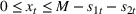
We consider an 


In any given year, crop planning for the next year starts immediately after the harvest in late fall (HGoA, 2018). Given the updated probability distributions for the yields of hops and the conventional crop, as well as the probability distribution representing the uncertain market demand, prior to the start of each year the farmer must make two sets of planning decisions: The farmer must determine how many acres of land to allocate to hops. This The farmer must determine the intended allotment level, that is, the maximum amount of hops production over the next year that will be contracted to brewers. In making this
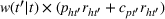
Once the allocation and allotment decisions are made for the next year, the farmer will advertise his hops to local brewers and start accepting orders (or signing forward contracts with potential buyers). The total demand for hops from brewers will be denoted by 


Actual crop planting (performed according to allocation decision made in the previous fall) and growing begins in late spring and continues until the fall harvest for both hops and conventional crops. During the harvest season, the farmer fills the brewers' orders for hops based on a first‐reserved, first‐served policy. The harvest season is typically fairly short. The hops, once harvested, need to be dried and well‐maintained, and wet hops can go bad within 1 or 2 days of the harvest. If there is an overage, that is, if the realized output is greater than the contracted orders, the farmer will sell the excess hops on the national spot market or to an agent who may possess better processing and storage capacity.
3
Given the small amount produced (and leftover after filling contracted orders) by the small farmers that motivate this research, it is unlikely that an individual farmer's production will affect the national spot market price. Thus, we model the spot market price as an exogenous random variable 


On the other hand, if there is an underage, that is, if the farmer cannot fill all of the contracted orders, the farmer will incur a penalty cost per pound, denoted by 


For conventional crops, we assume that the farmer can sell his entire output to the spot market at a price of 


Once the contract fulfillment process is complete, the farmer will move onto the next planning period, updating the probability distribution of the yield for each type of crop, and determining the additional hops acreage for the following year, as well as the allotment level.
Dynamic programming formulation
We next formulate a dynamic programming model for the farmer's problem, as described above.
System state
At the planning stage for the growing season in year 


Decision variables
The farmer must determine how many additional acres to allocate to growing hops, which we denote by 


State transition
The state transition is 


Profits per year
In year 


Given the realized demand (in pounds), denoted by If there is a underage, that is, if If there is an overage, that is, if 


For the conventional crop, without loss of generality, we assume there is no cost to prepare for planting. Therefore, the expected net revenue from the sale of the conventional crop in period 

The above cost and revenue expressions apply for years 
Dynamic programming formulation
The farmer's problem is to find the optimal allocation and allotment policies in each period to maximize the expected discounted profit over the 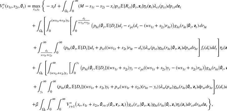


In this formulation, 


EXAMPLE OF LEARNING FRAMEWORKS
In this section, we introduce the KF as an example of a learning framework that can be used by farmers to update their knowledge of crop yields based on historical information and newly observed outputs. In Appendix A3 in the Supporting Information, we discuss another learning framework, the Bayesian linear model, and compare the two learning approaches.
The KF is a recursive procedure that iteratively uses observable outputs to obtain more accurate estimates of latent state variables. A KF consists of two types of equations, the measurement equations that describe how observed outputs are driven by latent state variables, and the state transition equations that describe the dynamic transition of state variables over time. Both the measurement and state transition noises are assumed to be normally distributed.
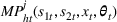
We use the model developed by Kaylen and Koroma (1991), where the crop yield follows a log‐normal distribution and the model parameters are the latent state variables that change over time. The measurement equation is equivalent to (1), but with 


The state transition equations can be written as 


The KF provides a way to dynamically estimate the state variables Suppose that the estimator


The predictive distribution of 


We only need to keep track of the most recent values, which can greatly reduce the state space. As 


The following corollary demonstrates that, for a setting in which the average annual weather condition stays the same between consecutive years, the dimension of the information state space can be greatly reduced. Although the average annual weather condition will typically change across years, the magnitude of this change is usually relatively small. Thus, Corollary 1 can be applied as a heuristic approach to simplify the state space and reduce the computational time. If the realized average annual weather conditions are the same for years 


Given Corollary 1, we can follow Farrell and Ioannou (2001) to develop a reduced‐order KF updating procedure, as shown below.


The information states for the above procedure are 


Finally, note that there is abundant literature discussing similar reduced‐order KF approaches. The approach used here, which follows Farrell and Ioannou (2001), is among the most highly cited. Further, as we demonstrate in Appendix A6.2 in the Supporting Information, this approach closely approximates the predictive crop yield estimates that are computed by the full KF procedure.
STRUCTURE OF THE OPTIMAL POLICIES
Next, we characterize the optimal acreage allocation and contract allotment policies. The optimal additional acreage to be allocated to hops production in year Given 


Proposition 2 implies that the optimal acreage allocation in a given year is a function determined by the total acreage currently allocated to hops, The optimal allocation decision, 


Corollary 2 supports the intuition that, if more acres have been previously allocated to hops, then less new acreage should be allocated to hops in current year. It also provides an upper bound on Consider a stationary setting, in which the probability distributions for the weather conditions and demand are constant over time. As the length of the planning horizon, 


Corollary 3 explores how farmers would behave in the long term when there is little opportunity to learn more about hops yield, that is, when they have obtained as much information as possible. In a stationary system, once the farmer becomes sufficiently experienced with hops yield, no additional acreage will be allocated and the total hops acreage in the long term will be constant.
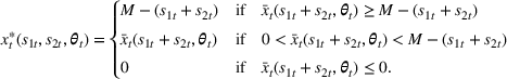
The following proposition characterizes the optimal intended allotment level decisions. The optimal hops contract intended allotment level for year 


The optimal allotment level is independent of acreage allocations, 


The following corollary indicates that a higher contracted price and a lower penalty cost for hops will encourage farmers to commit to provide a larger quantity of hops. The optimal intended allotment level, 


We next consider how the optimal allotment level varies as a function of the information state. Let 


Thus, the farmer should set a higher contract allotment level when the updated information state, as defined in Section 4, leads to a more preferable yield distribution.
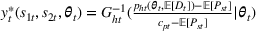
The following proposition implies that, as more acres are allocated to hops, the farmer will expect to see diminishing marginal profit per additional acre allocated to hops. The maximum profit‐to‐go in year 


Intuitively, when farmers sell hops to fulfill their contracted orders, the marginal profit per acre includes both the profit from selling the additional yield (generated by the additional acres) and the reduction in penalty costs from fulfilling more contracted orders, which is greater than the marginal profit of selling to the spot market. However, as more hops are grown, the chance that hops will be sold to the spot market in the future increases, leading to diminishing returns. When the marginal profit per acre allocated to hops becomes less than the marginal profit per acre of conventional crops, farmers will reserve the remaining acreage for conventional crop production. In Section 6, we present a heuristic solution procedure that makes use of Proposition 5.
The following corollary demonstrates that the farmer's profits will increase if the market has a higher hops contract price and decrease with a higher per‐unit penalty cost due to hops shortage. The maximum profit‐to‐go in year 


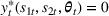
The following proposition demonstrates that, if a farmer has full knowledge of future crop yield distributions at the start of the planning horizon, that is, if the farmer does not need to update the crop yield distribution based on realized yields, then the optimal acreage allocation policy may allocate positive acreage to hops In the special case with no learning regarding crop yields, that is, when there is no need to track the historical data, 


Thus, it is the opportunity to learn about yields that may lead the farmer to increase his hops allocation over time. Intuitively, given that the acreage allocation to hops can only increase over time, it would seem that the only conditions under which it would be optimal to add hops acreage would be when the farmer becomes more optimistic regarding the yield of hops or more pessimistic regarding the yield of conventional crops. However, in Subsection 7.3.1, we will show that this is not always the case, that is, the farmer may allocate more acreage to hops when future yield observations are anticipated to be poor. Given these nonintuitive results, farmers need insights regarding the conditions that may lead to additional acreage allocation, which we present in Subsection 7.3.
LEARNING‐BASED MTP HEURISTIC
Proposition 5 demonstrates that, in any given year, as the number of acres allocated to hops increases, the MTP per additional acre allocated to hops decreases. Further, it is clear that additional acreage should not be allocated to hops if the MTP from doing so is less than the MTP associated with the last acre used to grow the conventional crop. Thus, the acreage allocation decision for a given year can be based on a comparison of the MTPs for the conventional crop and hops, where the MTP in a given year should be computed by considering the entirety of the
In contrast to the learning‐based monotone backward induction algorithm proposed in Appendix A4 in the Supporting Information, the learning‐based MTP heuristic uses a forward algorithm in which we obtain near‐optimal decisions starting with year 1 and moving forward (iteratively) to year 


For the conventional crop, for any future year 


For hops, the calculation of the MTP is more complicated due to the fact that the yield varies depending on the age of the hops, as well as the fact that the selling price depends on whether the hops are sold under the forward contract or on the spot market. We first calculate the total hops yields and contracted orders and determine whether any of the hops production will be sold on the spot market. In any given year For year Let For any future year, For any future year We can thus compute 


As more acreage is allocated to hops, that is, as 


When the decision‐making process moves from year 


To extend the heuristic to reflect uncertainty, we perform a simulation in which 


Finally, in Appendix A5 in the Supporting Information, we present an algorithm to implement the learning‐based MTP heuristic.
NUMERICAL STUDY
We next present a numerical study based on the case of a small farmer in Nebraska who recently started growing hops and who must plan the acreage allocation between hops and corn.
Experimental setup
We consider a 10‐year, 20‐acre farmland allocation problem given two crops, hops and corn, where the latter serves as an example of a conventional crop. In our experiments, we utilize two types of data, that is, crop data and weather data. In addition to the widely used USDA data and the weather data from the National Oceanic and Atmospheric Administration, we collected hops price, cost, and yield information from the small farmer in Nebraska. Also, following the practice of this farmer, we assume the hops contract price is constant over the planning horizon. We use the historical national market prices and nationwide weather conditions from 2008 to 2017 to calibrate the probability distributions of the hops spot market price and corn price. To model uncertainty in the growing season weather conditions, we used the county level weather data from 1960 to 2017 to fit empirical distributions for the temperature and precipitation. See Appendices A6.1 and A7 in the Supporting Information for details.
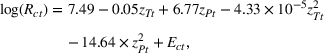
We use county‐level and national‐level data to fit the yield models for corn and hops, respectively. We obtain the following regression models, which we use as starting points for yield learning: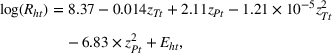


To reduce the computational complexity, we used the reduced‐order KF updating procedure introduced in Section 4 for all numerical experiments in Section 7. Numerical testing indicates that this reduced‐order KF closely approximates the full KF, as demonstrated in Appendix A6.2 in the Supporting Information.
Finally, for a detailed description of the parameter calibration, solution procedures and simulation setup used in our experiments, the reader is referred to Appendix A6 in the Supporting Information.
Performance of the learning‐based MTP heuristic
In this section, we evaluate the effectiveness and efficiency of the learning‐based MTP heuristic by comparing the decision policies generated through the heuristic and the learning‐based monotone backward induction algorithm in Appendix A4 in the Supporting Information. For comparison, we develop a decision policy using the heuristic to loop over the entire state space for all periods and then obtain the expected profit of the heuristic policy by inputting the heuristic policy into (2), which we denote as 


We perform 10 replications, where each replication has 1000 randomly generated scenarios. For each replication, we obtain the minimum, maximum and average optimality gaps over the discretized state space, as shown in Table 1 in Appendix A6.3 in the Supporting Information. As can be seen, the average and maximum optimality gaps are less than 2.12% and 3.74%, respectively, and the heuristic is a much more computationally efficient approach to finding the acreage allocation and contract allotment policies. The difference in computational time is primarily due to the fact that the heuristic solves the problem in a forward manner without the need to obtain the optimal solutions for all possible state values, as in the backward induction algorithm.
Given the results, we will use the heuristic to perform our numerical experiments for the remainder of Section 7. We let 

Impact of yield learning
In this section, we demonstrate the impact of yield learning by studying how the optimal decisions and profits are affected by learning due to changes in realized yields and weather conditions.
Impact of yield realizations
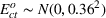
We first study how the farmer's decisions adapt to different yield realizations. In general, we find that a higher yield observation leads to a higher optimal allotment level. However, a higher yield realization does not always lead to a higher hops acreage allocation. In Figure 1, we demonstrate how the optimal decisions change for three different scenarios for the realized yields (as depicted in the top row of the figure). In the baseline scenario shown in Figure 1a, the realized yields are in the range of 1500–2000 pounds per acre per year. The low and high scenarios shown in Figure 1b,c have per acre realized yields that are 500 pounds lower and higher than the baseline scenario for each year. All other factors are the same for these three scenarios. The figure demonstrates that a higher realized yield leads to a higher optimal allotment level, which is consistent with the results in Proposition 4. For the acreage allocation decision, we see that the farmer will allocate 12 additional acres to hops at the start of year 1 under all three scenarios. Then, in year 2, the farmer allocates one additional acre under the baseline scenario, three additional acres under the low scenario, and four additional acres under the high scenario. These results may be due to the fact that the hops contract price is much higher than the hops spot market price. When the per acre hops yield is low, the per acre revenue earned from selling hops at the contract price could still be higher than the costs associated with the initial investment required for hops acreage, along with the opportunity cost of not growing corn. However, the same may not be true when selling at the (much lower) spot market price. Thus, the farmer may prefer to first fulfill the contracted hops demand and then grow corn with the remaining acreage. If a much lower‐than‐expected yield realization occurs, the farmer may not be able to meet all of the contracted demand. Thus, for the next year, he may choose to plant more hops in order to meet the more profitable contracted demand. However, when the per acre hops yield is sufficiently high, so that the per acre revenue from selling on the hops spot market can cover the investment and opportunity costs, the farmer will allocate more acreage to hops in order to meet both the contracted demand and spot market demand. Overall, these results demonstrate that, given the difference in prices for hops sold under contract versus the spot market, the differences in yield across maturity levels, and the uncertainty in both yield and demand, it is beneficial for farmers to use sophisticated decision‐making tools and yield learning, rather than intuition, to determine when to allocate more acreage to hops.
Optimal decisions for different yield observations. (a) Baseline. (b) Low yield observations. (c) High yield observations
Impact of weather changes
In Figure 2, we demonstrate how the acreage allocation and contract allotment decisions react to the changes in weather conditions. In Figure 2a, we show the baseline scenario in which the average growing season temperature and precipitation are fixed at 68.0°F and 0.10 inches, respectively, obtained based on historical weather data. Figure 2b,c incorporates a 3‐year temperature increase and precipitation drop, respectively, starting year 2, with all else remaining the same across the figures. Figure 2b suggests that, when the temperature increases, the farmer should allocate one more acre at the beginning of year 4, but allocate no additional acreage in years 2 and 3. In contrast, Figure 2c shows that, when the precipitation drops, the farmer should allocate one more acre in both years 3 and 4, while allocating no additional acreage in year 2. However, the farmer should decrease the contract allotment level immediately after either the temperature increase or precipitation decrease. Overall, the results demonstrate that, under yield learning and varying weather conditions, farmers should actively monitor and adapt to changes, adjusting their decisions based on realized conditions. In addition, we observe that the farmer adjusts the acreage allocation decision more cautiously than the contract allotment decision, due to the fact that the allocation decision has a more permanent and longer term impact on profits. For example, this figure indicates that the farmer should not change the allocation decision based on a one‐time change in the weather conditions, but should wait for more evidence of a permanent change. On the other hand, the farmer can use adjustments to the contract allotment level to cope with more short term changes to the weather conditions. Finally, note that while we demonstrate these insights through a single example, as shown in Figure 2, we explored a variety of other scenarios and observed consistent behavior.
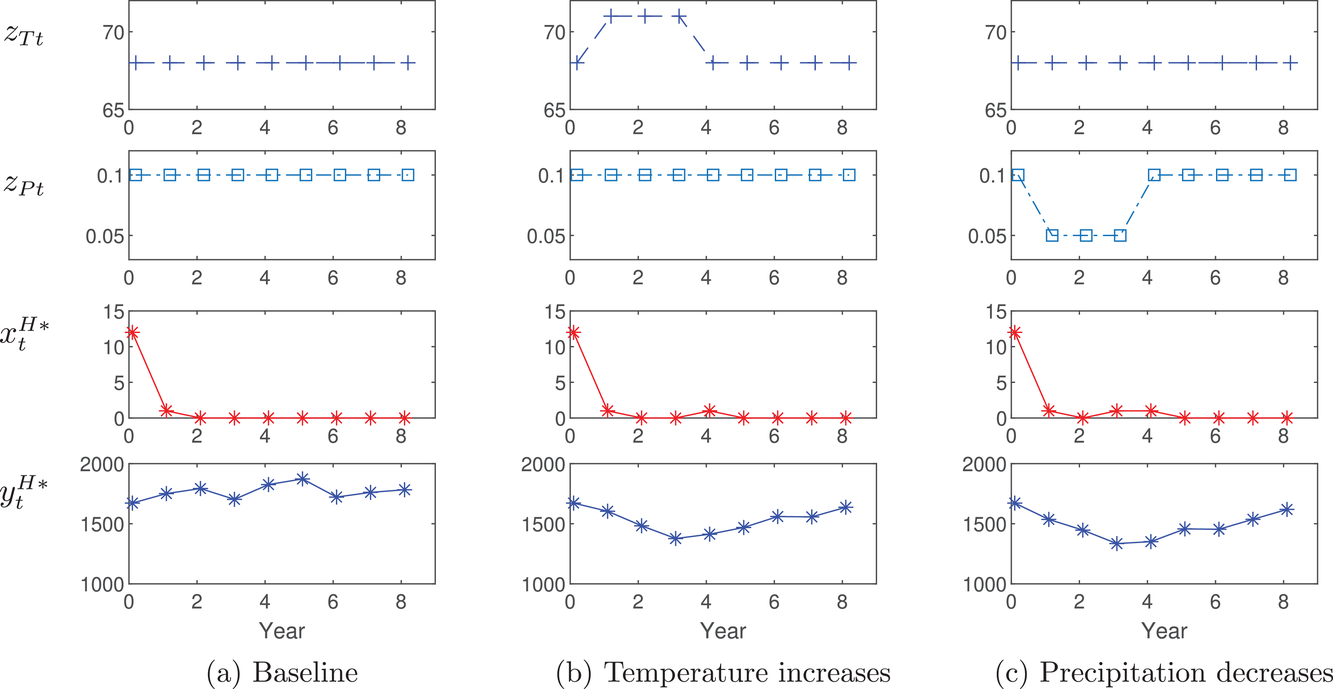
Impact of weather changes on allocation and allotment decisions. (a) Baseline. (b) Temperature increases. (c) Precipitation decreases
Impact of timing of a yield decrease
In Figure 3, we demonstrate how the learning framework reacts to a sudden decrease in the yield of hops, which may occur due to insect infestations and other natural phenomenon. In Figure 3a, we depict the baseline scenario in which the hops yield realizations are fixed at 1800 pounds per year. In Figure 3b,c, we show scenarios in which a sudden decrease in the realized yield occurs near the beginning of the planning horizon (year 2) and the end of the planning horizon (year 6), respectively, with all the other factors kept the same across the figures. The figure shows how the new hops acreage allocation and the optimal allotment levels react to the change in the yield realization. In Figure 3b, there is a sharp drop in the realized yield early in the planning horizon, resulting in one more acre allocated to hops in year 2. However, no additional acreage is allocated after year 2 since the realized yield returns to the baseline value, suggesting that it is important for the farmer to continuously monitor the realized yield. On the other hand, in Figure 3c, there is a sharp drop in the realized yield late in the planning horizon. In this case, by the time that the decreased yield realization occurs, substantial yield realizations have already been collected, and the model is less sensitive to a one‐time change in the realized yield. In terms of the farmer's actions, if a sharp decrease in the realized yield occurs early on, he will anticipate a lower future yield and will allocate more acres to hops than in the baseline scenario. However, if the farmer observes a sharp decrease in the realized yield later in the horizon, he may not react to this sudden change due to his experience with the historical yields. In addition, poor yield realizations that occur early in the planning horizon may lead the farmer to be more conservative and set a lower allotment level, while poor realizations later in the horizon have less impact on the allotment level. Finally, for the acreage allocation decisions, in contrast to Figure 2, which demonstrates that the farmer will have a delayed reaction to weather changes, the farmer should be more proactive in reacting to decreases in the yield.

Impact of a one‐time yield decrease on allocation and allotment decisions. (a) Baseline. (b) Early yield realization decrease. (c) Late yield realization decrease
Impact of prior distributions
This section investigates how the prior information used in the KF model will affect the farmer's decisions and profits. Specifically, we consider the means of parameters 


We first study the contract allotment decision 


Impact of prior mean on farmer decisions and profits. (a) Impact of mean of


The acreage allocation decisions 

Value of yield learning
In this section, we demonstrate the value of yield learning, which we define as the difference between the expected discounted net profits over the planning horizon obtained through the heuristic in Section 6 for the following two cases: the learning case, in which the model parameters are updated based on new yield realizations and weather observations, and the no‐learning case, in which the model parameters are assumed to be fixed at their prior values (i.e., their values at the start of the planning horizon). We find that, for the base parameter values, using the prior information obtained through historical data, as described in Subsection 7.1, the farmer can generate a total expected discounted profit of $857,420 over a 10‐year horizon for the learning case, which is a 75.7% increase over the no‐learning case. That increase is equivalent to a yearly profit increase of 6.4%, compounded annually. Further, the dollar value of yield learning for the base setting is $369,418.
We perform a sensitivity analysis to understand how the value of yield learning varies with respect to different prior distributions for the learning parameters, that is, with respect to the means and variances of the parameters 


Value of yield learning as functions of prior means. (a) Value of learning versus mean of


Value of yield learning as functions of prior variances. (a) Value of learning versus variance of


We also study the value of yield learning under different parameter settings to understand when yield learning will be most beneficial. In Figure 7, we demonstrate how the value of yield learning varies with respect to the mean of the hops contract demand, the hops contract price, the mean of the hops spot market price, and the mean of the corn price. We find that the value of learning is highest when the contracted demand is small. In particular, the value of learning decreases significantly, and then increases slightly, as the demand grows. Further, as the hops contract price increases, the value of learning increases. This indicates that yield learning can be particularly beneficial when the farmer is considering whether to take advantage of the opportunity to invest in a high margin, but potentially risky, new crop such as hops. In contrast, the value of learning decreases with respect to the means of the hops spot market price and the corn price, although the rate of decrease is substantially higher with respect to the mean of the corn price. The small impact of the hops spot market price on the value of learning could be due to the fact that the farmer can use the contract allotment decisions to adjust the amount sold to the hops spot market, thus mitigating the impact of the spot market price on the value of yield learning. The significant decrease in the value of learning with respect to the corn price is likely due to the fact that, when corn is highly profitable, the farmer will not allocate much acreage to hops, implying that the extent of his knowledge regarding the yield for hops becomes less important. Overall, the above results suggest that the farmer should make the effort to learn about the hops yield when the hops contract market is small and when the hops contract price is high. However, farmers may see less value from learning when alternative crops become more profitable.
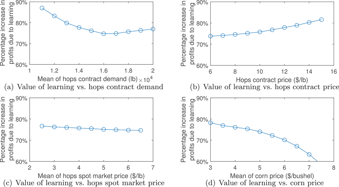
Value of yield learning under different demand and price settings. (a) Value of learning versus hops contract demand. (b) Value of learning versus hops contract price. (c) Value of learning versus hops spot market price. (d) Value of learning versus corn price
CONCLUSIONS
In this paper, we study the crop planning problem for a farmer who grows both specialty and conventional crops. This problem has become particularly important for farmers as they move to plant more valuable specialty crops to diversify their crop portfolio and hedge risks. However, planning for specialty crops can be challenging because they typically have distinctive characteristics (such as differing rates of maturity) and because farmers often have limited or no experience with these crops. Therefore, we investigate how a farmer should allocate the available acreage between hops (a type of specialty crop) and corn (a type of conventional crop), as well as how the farmer should set the contract terms (specifically, the intended allotment level) for hops under the commonly used forward contract for specialty crops. We develop a multi‐period stochastic dynamic programming framework, with the objective of maximizing the farmer's profit, which captures yield differences across maturity levels, yield correlations between hops and corn (through their dependence of common operating factors), and yield learning as farmers update their beliefs regarding future yields based on realized yields. We demonstrate our general model by discussing the KF learning framework, which is commonly used in the agricultural industry. We use our analytical results to develop a reduced‐form learning framework, which can significantly reduce the state space required for learning. Our analysis of the structure of the farmer's optimal allocation and allotment decisions suggests that the acreage allocation and allotment decisions can be separated, and that the allotment decisions can be determined using a closed‐form expression. In addition, we find that the acreage allocation decision depends only on the total hops acreage, rather than on the specific acreage of hops at the different maturity levels. Finally, we develop and implement a learning‐based heuristic that leverages the structural properties identified through our analysis. The proposed heuristic can significantly reduce the computational time, solving the entire problem quickly, which is critical for practical implementation.
Using data from the USDA and a local hops farmer, we performed a comprehensive numerical study. Our results demonstrate the importance of yield learning for specialty crop planning and provide practical insights to assist farmers in responding to varying weather and yield realizations. For a farmer with a 20‐acre farm and a 10‐year planning horizon, yield learning can contribute to a 6.4% yearly increase in profits compared to a setting with no learning. The value of yield learning is more substantial when the impact of temperature on crop yields is low, when the variances of a farmer's prior information are large, and when good initial estimates of the impact of precipitation on yield are not available. Farmers also benefit most from learning when the hops contract demand is low and when the hops contract price is high, but see less benefit when the hops spot market price and the corn price are high. We also find that farmers should use the acreage allocation decision to cope with long‐term weather changes and poor yield realizations early in the planning horizon, while they should use the contract allotment decision to handle more short‐term weather changes and poor yield realizations that occur later in the horizon. Finally, our results demonstrate that the optimal specialty crop planning policies are complex, indicating that more advanced decision support tools, such as the heuristic developed in this paper, are needed to assist farmers in improving their operations.
Finally, we discuss some limitations and potential extensions of our model and analysis. We assume that farmers are not able to convert acreage allocated to the specialty crop back to use for the conventional crop within the planning horizon due to the practical challenges associated with such conversion. However, there may exist situations, such as planning for other specialty crops, for which this conversion is less challenging. In such settings, our model would require significant modification, including the inclusion of a cost associated with acreage conversion, additional decision variables, and modified state transition dynamics. We believe that, if such acreage conversion is possible at a modest cost, the farmer would more aggressively invest in specialty crop production because it would be feasible to later convert the allocated acreage back to the conventional crop, if desired. On the other hand, if the conversion cost is sufficiently high, then our current results should hold. In general, we expect the conversion cost to be high due to the significant initial investment cost and the cost of removing the hops acreage. However, if the conversion cost is low, we would not recommend using our model. In addition, we do not consider the fact that the hops spot market price and the penalty cost due to hops shortage could be correlated with the focal farmer's hops yield. However, as we discuss in Appendix A9 in the Supporting Information, our structural results continue to hold when these correlations are considered, although a closed form solution for the contract allotment decision no longer exists. Practically, when there is a strong correlation between the hops spot market price (hops shortage penalty cost) and the focal farmer's hops yield, the farmer should consider increasing (decreasing) the hops acreage allocation and decreasing (decreasing) the hops contract allotment level if the farmer observes reduced hops production.
Footnotes
1
A number of other specialty crops, such as fruit trees, coffee, and cocoa beans, are also difficult and costly for farmers to remove once planted. For example, many types of fruit trees, including apple, cherry and pear, are difficult to remove, considering the significant investment required to plant them, the cost of removing the roots, and lost future revenues given that they have a life expectancy of several decades (Barth, ![]() ).
).
2
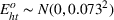
The notation ![]() ), and pears (Prengaman, 2022).
), and pears (Prengaman, 2022).
3
References
Supplementary Material
Please find the following supplemental material available below.
For Open Access articles published under a Creative Commons License, all supplemental material carries the same license as the article it is associated with.
For non-Open Access articles published, all supplemental material carries a non-exclusive license, and permission requests for re-use of supplemental material or any part of supplemental material shall be sent directly to the copyright owner as specified in the copyright notice associated with the article.