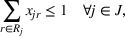
As the ongoing battle between brick‐and‐mortar stores and e‐commerce shops escalates, managers of the former are becoming more cautious regarding their strategic store site selection and decoration decisions, particularly if foreseeable competition from rival companies exists. This paper investigates a bilevel competitive facility location (BCFL) problem, where two companies, a leader and a follower, plan to enter a market sequentially. Each company has a budget to open and design facilities. The goal is to maximize expected revenue that is forecasted through a discrete choice model. To reflect a practical environment, we further consider a situation with elastic demand, explaining the market expansion effect when customers are offered better service due to the opening of new facilities. We formulate the problem as a nonlinear 0‐1 bilevel program. Because of the bilevel structure and the market expansion effect, this problem is so challenging that we are unaware of any exact algorithms in the literature. Motivated by this gap, we develop an exact framework that leverages the state‐of‐the‐art value‐function–based approach. However, this framework requires solving a mixed‐integer nonconvex optimization problem (MINOP) at each iteration, which is computationally prohibitive even for medium‐scale instances. To mitigate the intractability, we propose a new framework that avoids MINOP and tackles instances with hundreds of location variables. Finally, we conduct extensive computational studies to show the efficiency and effectiveness of our method as well as provide insightful guidance for managers to have win–win/dominate outcomes and choose an appropriate market size function when dealing with expansion decisions in chained business operations.
Market competition, under proper circumstances and regulations, has the power to make a business better serve its customers. Sportswear retailing brands, for example, Adidas and Nike, always have their stores sit closely to each other in order to satisfy customers' diverse requirements and, where possible, cannibalize the rival's market share. In fact, market competition is inevitably found in most business environments, whose occurrence has been partially explained by the median voter theorem from economists' lens (Downs, 1957). Essentially, any company that strays too far from customers at the business center will soon be out of business. Therefore, it is common to observe that the above sportswear twins keep their presence nearby at popular shopping malls.
Undoubtedly, the athleisure industry has boomed over the last few years, wherein the competitive store locations are certainly of strategic importance to determine the sales and operational costs. Consultants estimated that it costs approximately USD 107,500 on average to open a brick‐and‐mortar sportswear retailing store, in which the rental and decoration components account for over 80% in total (CostHack, 2021). As is commonly known, location plays a key role in attracting and retaining customers—a good location decision can significantly boost a store's long‐term sales performance while unwise decisions might result in loss of customers costing up to thousands of dollars. Retail store decoration, without a shadow of doubt, also has a tangible and far‐reaching impact on securing customers and, perhaps more importantly, allows differentiation from its competitors. Thus, executive board members are more than cautious to locate new physical stores and decorate them with different budget levels when planning to enter a new market. For example, in 2019, Adidas opened 147 new stores in total, among which, 142 were decorated as factory outlets and 5 as concession corners stores; meanwhile, it also closed 9 concept stores (Statista, 2021). A similar emphasis on physical stores' decisions was also identified in Nike's business practice (Emma, 2019). As large companies face site selection and decoration decisions, a natural question that arises concerns about how a company such as Adidas locates and designs its new store by anticipating the potential competition from its competitors (e.g., Nike) in the near future. In our opinion, this is an interesting topic that requires further contributive investigation.
Our study is motivated by the site location and design problem in the athleisure retailing industry, which is somewhat affiliated to the competitive facility location (CFL) problem. The CFL is a vibrant research field that studies an “entrant” company planning to enter a market with incumbent or prospective competitors. The company wishes to locate and design new facilities to maximize the expected market share (or revenue) that is characterized by discrete choice models (e.g., multinominal logit model and gravity model), given different competition types enforced by the competitors. Particularly, previous literature illustrates CFL models in terms of two streams, static versus foresight. The former assumes that the competitor's facilities location and design decisions are not affected as the company enters the market (Lin & Tian, 2021b; Ljubić & Moreno, 2018). The latter, on the contrary, takes the competitor's reaction into consideration. Such a problem, often termed as CFL with foresight, has been developed from a game‐theoretical perspective and is inherently more challenging than its static counterpart. We suggest interested readers to the book by Mallozzi et al. (2017) for a comprehensive discussion. Zooming on CFL with foresight, there are two main branches in terms of reaction timing, that is, simultaneous‐ and sequential‐entry CFL. According to the literature on simultaneous‐entry CFL, competition is embedded into a Nash game where companies simultaneously make the location and design decisions on their own facilities. Under Nash equilibrium, no company can improve the market share/revenue by unilaterally altering its own strategy. However, such an equilibrium is absent in many cases. In contrast, the sequential‐entry CFL problem assumes that there exists a “leader” that makes decisions at first and interprets the problem as a Stackelberg (leader–follower) game. More precisely, the leader needs to anticipate the reaction of the follower(s) so as to select the best strategy, thereby leading to a bilevel optimization program (Wu et al., 2016; Xiong et al., 2021).
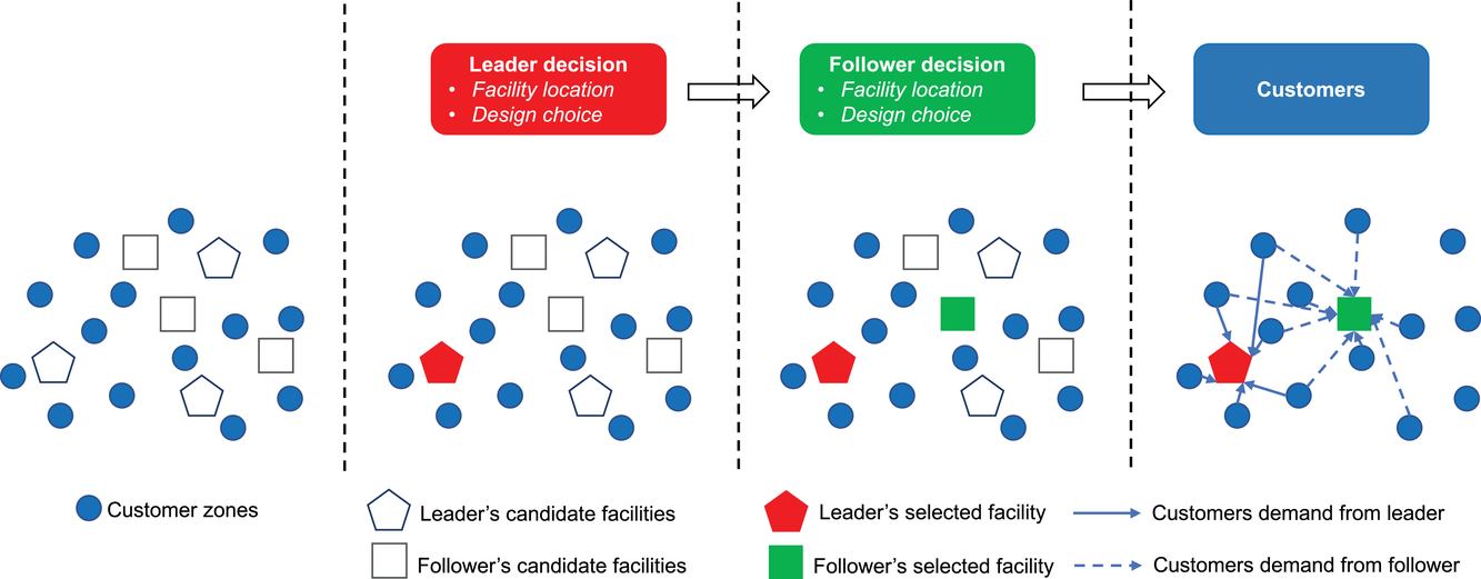
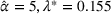
In this paper, we focus exclusively on the sequential‐entry setting and consider the bilevel competitive facility location (BCFL) problem with two competing companies, that is, a leader and a follower. Below, we describe the detailed BCFL decision process as shown in Figure 1. Suppose that each company has a fixed amount of budget to set up and design the facilities (i.e., rectangle and pentagon). In addition, each facility has several design options that exhibit different utility levels to the customers and incur different costs. Sequentially, the leader and then the follower are required to locate and design new facilities at candidate sites (i.e., filled rectangle and pentagon). The goal of each company is to attract as many customers as possible, that is, to maximize the expected revenue (sum of fractional weights on solid or dash arrows).
Illustration of a BCFL‐VM problem in discrete space
This paper further considers the market expansion effect, a concept that has been gaining considerable research attention in recent operational studies related to customer choices (Baloch & Gzara, 2020; Lin & Tian, 2021c; Wang, 2021). It is commonly assumed that the market size is influenced by the companies' decision, and empirical evidence has demonstrated that failure to account for the variable market size may result in substantial loss (Wang, 2021). In previous CFL studies, it has been reported that when companies open new facilities, customers will experience or perceive better service quality or utility, causing demand volume to increase (Berman et al., 2009). It is indeed a spillover phenomenon induced by the economies of scale and a direct consequence of the bandwagon effect (i.e., a popular trend attracts even greater popularity). However, most extant studies mainly focus on single‐level models (i.e., static competition) while the market expansion effect has not been fully investigated in a Stackelberg setting. Furthermore, an interesting question regarding how the leader and follower split the incremental market size, such as the situations of win–win or winner‐takes‐all, has not been answered in the literature yet. Motivated by these observations, we adopt that both the leader and the follower will take the market expansion effect into consideration when making their decisions and intend to address the open question with a more insightful analysis.
In essence, we formally introduce a nonlinear bilevel competitive facility location problem with variable market size (BCFL‐VM) and formulate it as a nonlinear 0‐1 bilevel program. Clearly, the following three distinct features of the BCFL‐VM render it rather challenging to address exactly: (i) First and foremost, given the bilevel decision structure, the leader knows ex ante that the follower observes its decision before reacting optimally. Therefore, if the leader aims to find out the best strategy, then it needs to anticipate the follower's response in advance. (ii) Due to the restricted choices in a discrete space, extensive efforts are required to satisfy the integrality conditions. (iii) Last but not least, the variable market size incorporates additional customer behavior factors and interactions into the nonlinear decision objectives, thereby leading to foreseeably extra computational iterations. To the best of our knowledge, we are unaware of any exact solution approach in the BCFL literature that can handle such a problem in possession of the aforementioned features in practical business environments. In light of these observations, this paper is dedicated to developing a high‐performance exact algorithm to search for solutions of proven optimality, which is also generalizable to address other industrial decisions.
Because the decisions related to location and design are strategically long‐lasting and economically prohibitive to alter for years, we identify a wide variety of applications for our proposed approach in business environments. For example, when the U.S. retail giant Walmart debuted its business in London, as an incumbent, it had to anticipate that other retailers (e.g., Tesco and Marks & Spencer) would enter the nearby regions and compete for market share soon. Another interesting application of the BCFL‐VM is in the context of chained business decisions among hotels (e.g., Hilton and Marriot) and shopping malls, in which the manager needs to make a strategic facility deployment and design plan with the foresight of its competitor's (enter)response.
Related literature
We briefly review related works regarding BCFL solution approaches to position the contributions of this paper. To date, many BCFL solution methods are heuristics, which rely on metaheuristic methods (e.g., tabu search, randomized local search, and evolutionary algorithm) to search for improved leader solutions. The quality of a leader's solution is evaluated by solving a follower problem (Biesinger et al., 2015; Drezner et al., 2015). However, these methods are not guaranteed to find an optimal solution and require solving the follower problem for a large number of iterations. Considering that the follower problem itself is possibly NP‐hard (in many cases, it is a static CFL), the effectiveness of these approaches is also limited. As a result, nonexact algorithms or metaheuristics have been adopted to solve the follower problem in a computationally efficient manner (Biesinger et al., 2016).
There exists a considerable number of works on linear BCFL, which assumes that customers only visit the most attractive facility. The resulting models are bilevel linear 0‐1 programs. This research stream is also called the discrete
‐centroid problem where several exact solution approaches exist. By representing the model as a maximization problem of a pseudo‐Boolean function, Beresnev (2013) proposed an exact branch‐and‐bound algorithm, which was later extended to solve the case where the facility capacity was considered (Beresnev & Melnikov, 2018). However, as shown in the study, such a method can only handle small‐scale instances with less than 35 possible locations in a reasonable time. Alekseeva et al. (2015) presented an integer linear reformulation using an exponential number of constraints. Based on this representation, they developed an iterative algorithm that combines with a local search procedure to search for a feasible solution given certain constraints. Gentile et al. (2018) also restated the model as an integer linear program. Different from Alekseeva et al. (2015), the formulation was solved via a branch‐and‐cut algorithm where the cuts were generated on‐the‐fly by solving some separation problems.
The exact methods mentioned above are dedicated to linear BCFL models, assuming that customers make deterministic choices. However, it is prevailing in the CFL literature that customer's choices are captured probabilistically (Berman et al., 2009; Ljubić & Moreno, 2018). This is because an individual may prefer a facility that is not necessarily the nearest according to their preferences. These preferences are typically unknown or hard to measure; therefore, the odds of a customer patronizing a facility should be estimated by some probabilistic choice models. This argument has been well supported by empirical evidence and validated through big‐data analysis (Lyu & Teo, 2022; Suhara et al., 2021). In this paper, we consider a BCFL model with a proportional choice rule based on Luce's choice axiom (Luce, 2012), leading to a nonlinear BCFL model that is fundamentally different from the linear case. Furthermore, we explicitly consider the market expansion effect, which is an important but usually neglected aspect, making the resultant model even more challenging than the linear BCFL models.
To the best of our knowledge, the only exact approach for nonlinear BCFL was proposed by Küçükaydin et al. (2011) for addressing a special case of the problem. They considered that the leader makes both discrete location decisions and continuous design decisions for the facilities, whereas the follower has already set up the facilities and the decision is to make continuous adjustments in the design of facilities. The follower problem was a convex optimization problem. With Karush‐Kuhn‐Tucker (KKT) conditions, the bilevel model was recast into a non‐convex mixed‐integer program (NMIP), which was subsequently solved to α‐optimality using the GMIN‐αBB algorithm (Adjiman et al., 2000). However, there are two main limitations. First, this approach cannot be used to solve the problem where both companies make location decisions. If the follower problem contains discrete variables, then the KKT conditions are not applicable. Second, the KKT‐based reformulation leads to an NMIP whose nonconvexity makes it computationally prohibitive even for small‐scale problems. In the numerical experiment, GMIN‐αBB can only solve problems with less than 20 leader facilities and 8 follower facilities.
To address the aforementioned gaps, we aim to develop an exact approach for large‐scale nonlinear BCFL problem. Our methodology certainly contributes to the research stream on (mixed‐)integer bilevel optimization. In particular, the majority of extant studies in this regard focus on linear problems, where both the objective functions and constraints are linear, and branch‐and‐cut algorithms are considered as state‐of‐the‐art techniques (Fischetti et al., 2017; Tahernejad et al., 2020). This situation aligns with the literature on linear BCFL where, indeed, efficient exact algorithms were implemented within branch‐and‐cut frameworks. We refer the readers to Kleinert et al. (2021) for a comprehensive survey on bilevel optimization. However, upon departing from the extant literature and incorporating nonlinearity, the corresponding bilevel problem becomes extremely challenging. Although several algorithms have been proposed—for example, the branch‐and‐sandwich approach by Kleniati and Adjiman (2015) and the iterative framework by Mitsos (2010)—due to extra efforts required to handle the nonlinearity (even nonconvexity), these algorithms were shown to be limitedly effective and only tested with small‐scale instances. Recently, Lozano and Smith (2017) proposed a powerful value‐function–based approach that can handle both optimistic and pessimistic versions of the bilevel problem. Motivated by this framework and underpinned by various acceleration procedures and reformulation techniques, we design a more powerful solution framework that substantially enhances the computational performance.
Our contributions
Our main contributions include the hierarchical problem definition, (enhanced) exact methods development, as well as insights from numerical experiments.
Hierarchically strategic decisions with distinct features. This paper investigates nonlinear BCFL with discrete location and design decisions for both the leader and the follower under variable market size. Such a BCFL‐VM problem is inherently more challenging than linear BCFL, nonlinear BCFL with continuous decision variables for the follower, and nonlinear BCFL without market expansion effect.
Exact methods and acceleration enhancement. To the best of our knowledge, although there exists a large body of research on nonlinear discrete BCFL, the exact solution approach to address nonlinear BCFL with variable market size is still absent. Motivated by this research gap, we develop the following two exact solution frameworks:
VF‐based algorithm. The algorithm is motivated by the state‐of‐the‐art value‐function reformulation approach. Specifically, we craft the framework of Lozano and Smith (2017) to align with our problem setting and derive an iterative algorithm that alternates between an upper bounding problem and a lower bounding problem.
EVF‐based algorithm. As the upper bounding problem is a mixed‐integer nonconvex optimization problem (MINOP), it becomes a key bottleneck to the solution procedure. We thus propose an enhanced version of the VF‐based framework, in which both bounding problems show convex structures and can be solved significantly faster. To efficiently solve the bounding problems, we develop branch‐and‐cut algorithms based on outer‐approximation (OA) cuts and customized conic approaches leveraging the second‐order conic representability of the problems.
Insights from experimental tests. We test the performance of the algorithms on a broad testbed. The results show that our enhanced algorithm is rather effective and that it can yield significant improvement with up to several orders of magnitude in terms of computational time compared to the original framework by Lozano and Smith (2017). Furthermore, when the market size is fixed, our algorithm can satisfactorily handle instances with hundreds of location variables in a reasonable computational time. Our tests also provide several managerial insights for chained business decisions in terms of typical design parameters such as budget, demand elasticity, and choice‐set characteristics. For example, we conclude that the unilateral raising budget activity will lead to a “win‐win” or “raiser dominates” outcome, depending on the trade‐off consequence between spillover and cannibalization effects in a concavely sized expanded market. In addition, we find that adopting a well‐fitted market size function can significantly reduce potential revenue loss and help managers achieve more desirable expansion results.
The rest of the paper is organized as follows. We present the problem description and the model for the BCFL‐VM in Section 2. Then, we develop an exact solution algorithm based on the value‐function reformulation approach in Section 3. Section 4 presents an enhanced algorithm that substantially speeds up computation time. We then conduct extensive computational studies and discussion in Sections 5 and 6, followed by a concluding remark in Section 7.
PROBLEM DESCRIPTION
Basic setting
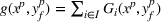
This section presents a detailed description of the problem. Two companies, a leader and a follower, are planning to enter a market. The leader and the follower will locate and design new facilities among a few candidate sites sequentially. For example, in Figure 1, the pentagons represent the candidate locations for the leader while rectangles denote potential locations of the follower. It is assumed that when a facility is open, it is able to attract a certain number of customers to visit (e.g., the opening of a new shopping mall). Moreover, each facility has several design options that exhibit different utility/attraction levels to the customers and incur different costs. With a fixed amount of budget, the goal of each company is to compete for attracting customers, that is, to maximize the expected revenue jointly determined by a market size function and a discrete choice model. More precisely, when customers are offered a set of open facilities from the leader and the follower, they first decide whether to use the service from one of the companies (which is predicted by a market size function). If yes, they subsequently choose a facility to patronize following the Luce's choice axiom (Luce, 2012). That is, the probability of a customer patronizing a facility is proportional to the utility/attraction provided by the facility to the customer. Notably, two popular models that exhibit such a proportional choice characteristic are the gravity model and the multinominal logit model, both of which have been widely adopted in the CFL literature (Aboolian et al., 2007; Drezner & Drezner, 2017; Freire et al., 2016; Ljubić & Moreno, 2018). Once the choice probabilities have been estimated, the expected revenue captured by a (leader or follower) company can be derived as a weighted sum of the market sizes among all demand zones multiplying the revenue produced by one unit of market size.
The market size at each customer zone is elastic, that is, we consider the market expansion effect, which states that when companies open new facilities, customers will experience or perceive better service quality or utility, and the demand volumes increase correspondingly. In the CFL models, this effect is typically defined as demand elasticity, and the demand volume or the market size at a customer zone is modeled by some expenditure function or market size function, which is assumed to be concave and nondecreasing over the total utilities that customers observe (Baloch & Gzara, 2020; Berman et al., 2009; Lin & Tian, 2021c).
Based on the above setup, we study a BCFL problem where the leader locates facilities first and the follower observes the leader's decision before responding in an optimal manner. Both companies make decisions considering the customer's choice behavior and the market expansion effect. We take the perspective of the leader and aim to find its best strategy for revenue maximization.
Model formulation
As indicated in Figure 1, we divide the region into several customer zones (circles) denoted by set I, and each zone aggregates the buying power
inside. The leader has a budget
that can be used to open the facilities, selecting from some candidate sites, that is, set J. When the leader opens facility j, there are
design options, and exactly one option will be chosen at the end. If an option
is selected, then the attractiveness of the facility j is denoted as
and, accordingly, the leader incurs a fixed cost
,
.
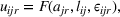
The utility of leader facility j under design option r to customer zone i is characterized by
where
is a nonnegative utility function that is assumed to depend on the attractiveness
of facility j with option r, the distance
between a facility j and a customer zone i, and an additional term
capturing the impact of other factors on the utility. On the one hand,
is an increasing function over
, meaning that when the leader invests more on facility j, the utility of the facility to customer zone i will increase. On the other hand,
is a decreasing function in
, suggesting that when the distance between the facility and the customer zone increases, the facility becomes less attractive.
Similarly, the follower has a budget
and its candidate facilities are denoted by a set K. There are
design options for facility k,
, and the attractiveness is
with a fixed cost
,
. We then describe the utility of follower facility k under design option r to customer zone i by
where
is a nonnegative utility function that depends on
, the distance
between facility k and customer zone i, and an additional term
.
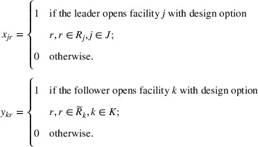
Now, we define two binary variables
and
that are required for model development:
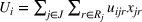
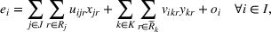
Given this, for a customer zone i, the total utility
from the leader facilities and the total utility
from the follower facilities are defined as
and
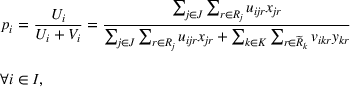
. According to the proportional choice rule, the probability of a customer at zone i patronizing one of the leader's facilities is given by
where the denominator stands for the total utility jointly provided by the leader and the follower to customer zone i. We define
to emphasize that such total utility is determined by the decisions of both companies, that is,
Similarly, the probability of a customer at zone i patronizing one of the follower's facilities is given by
.
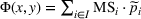
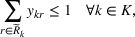
The market size at zone i is assumed to be elastic and represented by some expenditure function
over the total utility, that is,
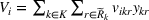
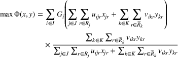
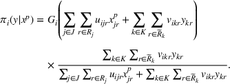
In this paper, MSi can be interpreted as the number of customers at zone i that will eventually patronize the facilities opened by the leader and the follower. For ease of exposition, we assume that one unit of market share leads to one unit of revenue. Given the market size, we estimate the revenue of the leader as
and that of the follower as
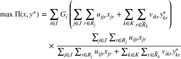
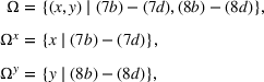
. With these notations, BCFL‐VM can be formulated as the following bilevel optimization problem:
where
is an optimal solution to the follower problem.
Objective functions (7a) and (8a) are the revenue of the leader and the follower, respectively. Constraints (7b) and (8b) are their budget restrictions. Constraints (7c) and (8c) ensure that only one design option can be selected if a facility is open. Finally, constraints (7d) and (8d) are the integrality restrictions on the decision variables. We refer to the above bilevel model as the nonlinear BCFL‐VM.
In the BCFL‐VM model, the utilities of the leader and the follower facilities are represented by (1) and (2). Both equations impose that the utility should increase with the attractiveness of the facility and decrease with the distance between the facility and the customer zone. Gravity‐based utilities exactly satisfy these requirements and have been validated in various empirical studies (Drezner, 2006; Suhara et al., 2021). We therefore adopt the gravity‐based utilities function in this paper. For simplicity, we also set
and
to 0 so that the utility only depends on the attractiveness of the facility at a specific design option and the distance, that is,
, where
is a distance decay function that reflects the decline in the probability of a customer patronizing a facility as a function of his/her distance away from the facility. We note that our model is not restricted to the gravity‐based utility. Instead, it can be extended to other types of utility functions as the utilities are input parameters (and not decision variables). In real‐world applications, the utility shall be estimated from a practical data set and its formulation depends on a specific business environment under investigation.
Market size function
With variable market size assumption, customers' choice behavior can be illustrated as follows. When companies open new facilities, customers are expected to determine whether to use the service from the companies at first. If not, the demand is lost from the companies' perspective; if yes, they subsequently select an open facility to patronize following the proportional choice rule.
Given the above procedure, the market size function comes into effect to specify the total number of customers that are attracted by the leader and the follower. In particular, it also reflects the “demand loss” scenario when a customer decides not to use the service from the companies. Following the common assumption on market expansion in the CFL literature, we represent the market size in (6) by concave expenditure functions that are nondecreasing in the total utility (Berman et al., 2009). Considering the variable market size assumption and the demand loss scenario, two types of expenditure functions arise for general purpose.
Fractional expenditure function (FEF), which takes the form
where
is the maximum possible demand at zone i and
is a nonnegative parameter that can be interpreted as the utility of “not‐use‐the‐service.” The demand loss is captured by a fractional term
. In the extreme case where
, the demand loss is zero. The demand becomes inelastic and thus attains its maximum level, that is,
.
Exponential expenditure function (EEF), which is represented by
where
is a parameter that reflects both the elasticity and the size of demand with respect to the total utility. The demand loss is given by an exponential term
. When the value of
is higher, the demand is larger. Specifically, when
, the demand becomes inelastic and attains its maximum level, that is,
. Such a function has been widely used in various static CFL models to capture the market expansion effect (Aboolian et al., 2007; Baloch & Gzara, 2020).
In general, under the above expenditure functions, the follower's objective
is either a convex or a concave function. Fortunately, the following lemma establishes the concavity and convexity of
when we fix the leader's decision and the follower's decision, respectively.
Under FEF and EEF, we have the following results. (i) If the leader's decision is fixed at
, then
is a concave function over the follower's decision space y. (ii) If the follower's decision is fixed at
, then
is a convex function over the leader's decision space x.
We present the proof in Supporting Infomation EC.1. Note that this lemma serves as a key component in developing the solution algorithms for BCFL‐VM in Sections 3 and 4.
Last but not least, it is worth noting that there is a possible variant of the BCFL‐VM, that is, we can further consider an explicit exit option to represent a scenario when customers do not select any facility from both companies. Specifically, let
denote the utility of this option for customers in zone i. We may redefine
and MSi as
and
, respectively. The exit option has been investigated in choice‐based operations management (Wang, 2021) under the static competition. However, in the BCFL literature where there exists Stackelberg competition between two companies, it is commonly assumed that when the market size is fixed, the demand is fully captured by the leader and the follower (Beresnev & Melnikov, 2018; Biesinger et al., 2016; Drezner et al., 2015; Gentile et al., 2018; Kochetov et al., 2013; Küçükaydin et al., 2011). Otherwise, it implies that there is a “third company,” implicitly competing with the leader and the follower in a static manner (because, oftentimes, the exit option can be interpreted as “seek‐the‐service‐from‐alternatives”). Essentially, the demand loss caused by the exit option has been captured by the aforementioned market size function. Hereafter, aligning with the mainstream among the BCFL literature, we do not consider the exit option explicitly. Nonetheless, we point out that when the market size function follows FEF, our proposed modeling framework and the subsequent solution algorithms can be directly applied to the problem with an explicit exit option after a slight modification of parameters definition. For the case of EEF, the model can also be extended at the expense of extra computational efforts. Both extension details have been discussed in Supporting Information EC.6.
VALUE‐FUNCTION–BASED ALGORITHM
Motivated by the recent development in solving bilevel programs, we develop an exact solution framework, leveraging the value‐function reformulation approach—see Fischetti et al. (2017) and Lozano and Smith (2017) for its recent applications. Overall, the framework reformulates the BCFL‐VM into a single‐level model with an exponential number of constraints that specify all possible follower solutions. However, solving the value‐function–based formulation can be computationally expensive due to its exponential constraint size. Therefore, we employ a relaxed formulation, consisting of a subset of follower solutions (called the recorded response set), to obtain a valid upper bound (UB). A valid lower bound (LB) is obtained by solving a follower subproblem, whose solution is used to enlarge the recorded response set and to potentially tighten UB. The algorithm proceeds until UB converges at LB or certain stopping criteria are met.
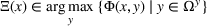
To facilitate our discussion, we define the following sets:
where Ω contains all possible decisions of the leader and the follower;
is the leader's decision space; and
is the follower's decision space. Next, we define
and
as the revenue of the leader and the follower, respectively. Furthermore, for each leader solution x, we define
as the follower rational response set, that is, the subset of follower solutions that maximize the follower's revenue given the leader solution x. In our problem, for every x, the follower's decision space is invariably
, that is, the leader solution does not make any follower decision infeasible, which is a common assumption in many nonlinear CFL models (Küçükaydin et al., 2011; Kochetov et al., 2013; Drezner et al., 2015). We call a solution
bilevel feasible if
and
. Note that if
is not a singleton, then y is chosen from
such that the market size is maximized. This is equivalent to indicating that if there exist multiple rational responses of the follower, then the follower will select the one that maximizes the market size.
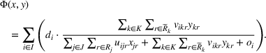
With the above notations, BCFL‐VM can be restated as
Note that the
in (13) is only known implicitly. Therefore, we reformulate (13) into an explicit optimization problem, supported by the following lemma.
A solution
is bilevel feasible if and only if
for every
.
This lemma is adapted from the established result in Ye (2006). The intuition is that for every
, if
, then y is optimal given the leader decision x and thus bilevel feasible.
Note that
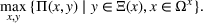
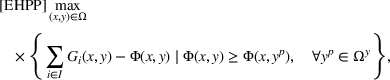
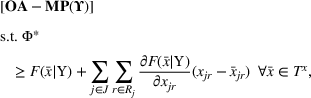
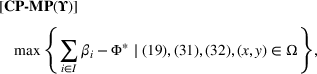
. Given Lemma 2, the bilevel problem (13) is reformulated as the following single‐level optimization problem:
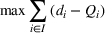
which is called the extended high‐point problem (EHPP). As the constraint of EHPP implies the optimality of the follower response given any leader decision x, that is, the constraint is equivalent to Equation (8a), the following result arises immediately.
EHPP is equivalent to BCFL‐VM.
Essentially, the formulation of EHPP suggests that if we can enumerate all feasible follower responses, then solving EHPP gives us an optimal solution of BCFL‐VM. However, the size of
could be exponentially large, and it is computationally unachievable to solve EHPP by fully enumerating all solutions in
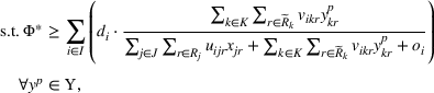
even for a moderate‐sized problem. Therefore, motivated by Lozano and Smith (2017), we consider a relaxation of EHPP, which only contains some (not all) feasible follower responses in the formulation. Specifically, we choose a response set Υ such that
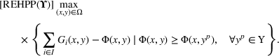
and use the following relaxed EHPP
Here, REHPP(Υ) stands for the relaxed extended high‐point problem. Let
be an optimal solution to REHPP(Υ). Because REHPP(Υ) is a relaxation of EHPP,
provides a UB to BCFL‐VM. In contrast, if a leader decision has been made at
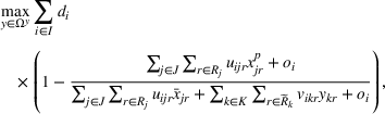
, then the follower will aim to maximize its revenue by solving the following problem:
Let
be an optimal solution to the follower subproblem, that is, FSP(
). As
is not necessarily optimal for the leader,
is of course an LB to BCFL‐VM.
To summarize, solving REHPP(Υ) and FSP(
) allows us to bound the best objective of BCFL‐VM from both upper and lower sides. Note that UB can be tightened if the response set Υ is enlarged. Therefore, through an appropriate way of generating new follower responses, it is possible to derive an exact algorithm that alternates between solving REHPP(Υ) and FSP(
) within finite iterations. This is exactly the procedure of Algorithm 1.
Value‐function–based algorithm for BCFL‐VM.
1:
Initialize ,
, and set counter
.
2:
Select a feasible leader solution x0. Solve FSP(x0) and obtain an optimal follower response
.
3:
Initialize the response set as
.
4:
while
do
5:
Set
6:
Solve REHPP(Υ). Obtain an optimal solution
. Set
.
7:
Solve FSP(
). Obtain an optimal follower response
. Set
.
8:
if
then
9:
The best solution
. STOP.
10:
else if
then
11:
Update
and the best solution
.
12:
Return
.
If REHPP(Υ) and FSP(
) can be solved optimally, then Algorithm 1 terminates in a finite number of iterations to an optimal solution of BCFL‐VM.
The proof is provided by Lozano and Smith (2017). Lemma 4 shows that this tailored value‐function–based algorithm can solve BCFL‐VM to the guaranteed optimality under finite iterations.
Despite having the finite convergence property, Algorithm 1 is computationally prohibitive for problems with a reasonable size.
is not concave over
in general; therefore, REHPP(Υ) is an MINOP, giving rise to a major bottleneck for the algorithm. In particular, when the market size is modeled by EEF, REHPP(Υ) cannot be solved efficiently using any existing approach, rendering Algorithm 1 practically ineffective for BCFL‐VM.
ENHANCED VALUE‐FUNCTION– BASED ALGORITHM
In this section, we develop another value‐function–based algorithm that subtly avoids handling REHPP(Υ) and instead solves a mixed‐integer convex master problem (20) to UB the objective. The new algorithm significantly improves computational efficiency. To complete the algorithm, we then propose both general and customized approaches for solving the follower subproblem (16) and the new upper bounding problem (20).
Overall framework
Due to the nonconcave term
, it is extremely challenging to solve REHPP(Υ). Observe that
appears both in the objective function and the constraint of REHPP(Υ). Moreover, in the objective, we seek to minimize
, whereas the constraint defines the lowest attainable value for
given the current response set Υ. This allows us to relax REHPP(Υ) by replacing
with a single variable
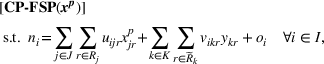
. Consider the following reformulated problem:
where the follower objective function
is replaced by
. We also define an intermediate variable
to represent the joint utility provided by the leader and the follower to customers at zone i, and write
in its hypograph form with the variable
representing the market size at zone i. Indeed, problem (17) is a convex problem because
Solving RP(Υ) provides a valid UB to BCFL‐VM. However, this UB may not be tightened to the optimal value. An intuitive explanation is presented as follows. Suppose that all
have been enumerated, an optimal solution of RP(Υ) is
in this setting. This is because, although the solution pair
is bilevel feasible and potentially optimal, the leader's objective in RP(Υ) could still be improved by choosing a
that leads to a larger market size, that is,
. In other words, due to the substitution of
by
, the linkage between the follower's response and the market size is lost. RP(Υ) thus may overestimate the market size in some scenarios because the follower's response is not explicitly considered in
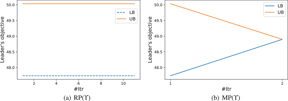
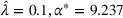
. Consequently, replacing REHPP(Υ) with RP(Υ) cannot ensure the convergence of the algorithm because the optimality gap may persist. As an example, Figure 2a shows the movement of LB and UB of a competitive facility location and design problem (CFLDP) instance (see the description in Section 5.1) with
. We can observe that starting from iteration 1, LB and UB do not change and the algorithm cannot converge.
LB and UB versus the number of iterations (# Itr) of a CLFDP instance when RP(Υ) or MP(Υ) is used as the upper bounding problem
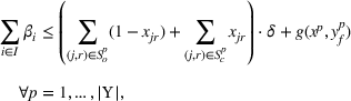
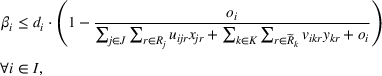
Therefore, we derive a simple but effective inequality to avoid the market size overestimation and remove the gap. Suppose that at iteration p, the leader's solution is
with an optimal response from the follower
. Then the true market size is given by
. Let
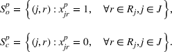
and
be the set of open‐design and not‐open facility decisions under solution
, that is,
We have the following linear constraint:
where δ is a large number. This constraint effectively imposes that the market size can be larger than
only if the leader's decision is not
. Otherwise, it will bound the market size at
, explicitly linking the market size with the follower response
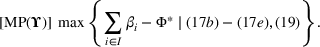
. With this bounding inequality, we propose the following master problem to derive the UB for BCFL‐VM:
Given MP(Υ), we design a new Algorithm 2, together with the proof of its finiteness, in Supporting Information EC.2. As reported in Figure 2b, Algorithm 2 (i.e., replacing REHPP(Υ) with MP(Υ)) requires only two iterations to verify the optimality of the solution.
In fact, Algorithm 2 is a modified version of Algorithm 1, and this modification yields significant enhancement (up to several orders of magnitude in terms of computational efficiency) as shown in Section 5. In brief, the merits of MP(Υ) are owing to its convex structure, which allows us to solve MP(Υ) much more efficiently than REHPP(Υ).
General branch‐and‐cut approach for MP(Υ) and FSP(
)
Note that Algorithm 2 terminates in a finite number of iterations to an optimal solution of BCFL‐VM, provided that MP(Υ) and FSP(
) can be solved optimally. However, both problems are not trivial. Hereafter, we will present their solution in detail.
Solving MP(Υ)
As MP(Υ) is a mixed‐integer convex optimization problem, we derive a branch‐and‐cut outer‐approximation (B&C‐OA) algorithm to solve it optimally. The fundamental idea of B&C‐OA is to maintain a single branch‐and‐cut tree and use first‐order OA cuts that are generated on‐the‐fly during the branch‐and‐cut searching tree to approximate the convex constraints (17b) and (17c).
We first generate OA cuts for constraint (17c). Given any solution
, because
is a concave function, we can UB it by its first‐order linear approximation, generated at
, that is,
Such a linear function will not eliminate any feasible region of MP(Υ) and further provides a valid cutting plane to cut off nonoptimal solutions.
We then continue to address constraint (17b). Note that during the iterations of Algorithm 2, new follower responses are added to set Υ, and they specify new nonlinear inequalities to constraint (17b), creating additional difficulties in modeling and solving MP(Υ). To derive a compact and unified OA cut, we first define a function
as
which expresses the right‐hand side of constraint (17b) under the current response set Υ into a single term. Note that
is a convex function, and thus function
is also convex as it is the maximum of
convex functions. For any solution
, we can then generate OA cuts at
as
where
is the partial derivative of
at
. More precisely, it can be computed as follows. Let
, then
, and we have
Now, given the OA cuts for constraints (17b) and (17c), we can describe MP(Υ) as the following mixed‐integer linear program (MILP) formulation:
where
and
are the sets of recorded
and
. These points define OA cuts that drive the solution to optimality. In this paper, we embed these OA cuts into the branch‐and‐cut procedure. Specifically, we use default branching rules and cutting planes in off‐the‐shelf MILP solvers and start by initializing problem (25) without OA cuts. While in the searching tree, once any integer nodes are identified, the corresponding solution
is retrieved. We then check if OA cuts (25b) and (25c) are violated by this solution up to a minimum relative violation of 10−5. If yes, we then expand
and/or
and add the corresponding OA cuts to the current LP relaxation as lazy cuts using the callback function within MILP solvers.
Solving FSP(Υ)
We proceed to introducing the solution approach for FSP(
) can now be solved using B&C‐OA following a philosophy similar to the one described to solve MP(Υ). That is, at the beginning, we solve the model (27) without constraint (27b). During the branch‐and‐cut searching tree, when an integer solution
that violates (27b) by a minimum relatively violation of 10−5 is identified, a cut (28) is added to the model.
Customized conic approach under FEF
In Section 4.2, we present B&C‐OA approaches to solve MP(Υ) and FSP
. These approaches are applicable to BCFL‐VM under both FEF and EEF and therefore provide a general framework for BCFL‐VM. Actually, when the market size is captured by the FEF, there exists a more efficient approach. That is, MP(Υ) and FSP
can be recast as mixed‐integer conic quadratic programs (MICQPs) and subsequently solved by modern MIP solvers. Conic program (CP) reformulation is an effective approach for solving fractional 0–1 programs and has been successfully applied to various facility location problems (Lin & Tian, 2021a; Lyu & Teo, 2022; Tiwari et al., 2021). Motivated by these studies, we present customized CP approaches for MP(Υ) and FSP
to expedite Algorithm 2 under FEF (a generic form of MICQP is provided in Supporting Information EC.3 for reference).
CP approach for MP(Υ)
Under FEF, the follower's objective is given by
As a result, the master problem can be written as
where we have two nonlinear constraints (30c) and (30b). We show that they can be reformulated as second‐order conic constraints.
Let us first study the reformulation of (30c). We define variable
To summarize, MP(Υ) is finally reformulated as the following program:
which has a linear objective function, and the constraints are either linear or conic quadratic. Therefore, it definitely is an MICQP.
CP approach for FSP(
)
Under FEF, the follower subproblem FSP(
) becomes
where we have a nonlinear objective function that is second‐order conic representable. Let us define variable
such that
. We can then rewrite the objective function as
. Let us then introduce a variable
such that
holds, and we can construct a rotated conic inequality
, meaning that FSP(
) is equivalent to the following MICQP:
In a nutshell, under FEF, we can replace the generic MP(Υ) and FSP(
) with respective reformulated problems (33) and (35) to accelerate the convergence process.
In Algorithm 2, when using the MICQP approach, we need to introduce additional constraints in the form of (32) to MP(Υ) to tighten UB at each iteration. This process is similar to the cutting‐plane algorithm where we can improve the efficiency of solving the problem by warm‐starting the solver with some feasible and/or high‐quality solution. In this paper, at iteration
, we warm‐start the MICQP model (33) with the bilevel feasible solution
. Through our preliminary computational test, we find that such a straightforward warm‐start strategy generally leads to substantial speed up compared to the case where warm‐start is not implemented.
COMPUTATIONAL EXPERIMENTS
This section presents the computational experiments and result analysis. The algorithms are programmed using Python on a 16 GB RAM macOS computer with a 2.6 GHz Intel Core i7 processor. The adopted solver is Gurobi 9.1.2. Without loss of generality, we assume that the number of design options for all facilities is the same, that is,
.
Throughout this section, we refer to the value‐function–based algorithm (i.e., Algorithm 1) as VF. When both REHPP(Υ) and FSP(
) are solved by B&C‐OA, the approach is named after VF‐OA. By contrast, when both REHPP(Υ) and FSP(
) are solved by the CP reformulation, the approach is called VF‐CP. Moreover, we refer to the enhanced value‐function–based algorithm (i.e., Algorithm 2) as EVF, and use EVF‐OA and EVF‐CP to denote the approaches employing B&C‐OA and the CP reformulation to solve MP(Υ) and FSP(
). We point out that under EEF, only EVF‐OA is applicable as REHPP(Υ) and MP(Υ) are not MICQP‐representable. However, under FEF, all approaches can be used to solve BCFL‐VM. The nonconvex term
in REHPP(Υ) can be reformulated exactly. We present the corresponding linear formulation for
in Supporting Information EC.4.
We now define the measurements that will be used in our later discussion:
denotes the computational time in seconds. By default, we impose a 1‐h time limit (i.e., 3600 s) for solving an instance.
stands for the relative exit gap in percentages when the whole solution process terminates, that is,
. In our default setting, an instance is considered to be solved to optimality if rgap is less than 0.01%.
is the number of iterations, which also specifies the number of times we successfully solve REHPP(Υ) or MP(Υ).
Testbed
Our testbed includes two data sets, both of which have been used in various CFL models.
CFLDP,1 which is a data set in the well‐known Discrete Location Problems benchmarks library. It consists of 50 points on a plane, that is,
. l and
are computed by the Euclidean distance. For each facility, there are three design options, that is,
. Therefore, the total number of location variables are 300. The values for a,
, d, c, and g are also provided. This data set was originally used by Kochetov et al. (2013), where the gravity‐based utilities are defined as
and
.
COMP,2 which has been used as a common testbed in the discrete
‐centroid problem formulated as a linear 0‐1 bilevel program (Alekseeva et al., 2015). This data set is considered to be one of the hardest data sets in the discrete
‐centroid problem, because the computational time for some instances can blow up to several hours. In this paper, we adopt 10 structured problem data with nonhomogeneous (weighted) demand. The reference numbers are 111w, 211w, 311w,…,1011w. For these problems,
,
. In addition,
, meaning that the budget constraints become
,
. To facilitate our discussion, we set
. Moreover, to adjust the data for our problem, we generate
and
from a uniform distribution between 1 and 5.
and
are measured by the Euclidean distance in 100 units. The gravity‐based utilities are characterized by power decay as
and
.
Result analysis under FEF
We start by discussing the computational results under FEF. To model the attraction of outside option
, we use the following equation:
where
and
are the average values of
and
, respectively. Parameter
controls the magnitude of the attraction of the outside option. If
, then
, such that the market size is inelastic and attains its maximum value
.
CFLDP results
By considering three values of α, that is,
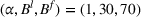
, we report the results of the generated 42 instances in Table 1. For each instance, the computational time for the approach that achieves the best performance (i.e., the smallest t[s] among VF‐OA, VF‐CP, EVF‐OA, and EVF‐CP) is highlighted in boldface. Given the table, we conclude the following observations.
Despite requiring additional iterations, the EVF‐based approaches are more efficient than the VF‐based ones in terms of computational time by orders of magnitude. All instances can be solved within 4 min by the EVF‐based approaches, whereas the VF‐based approaches typically require substantially long time and even fail to solve some instances optimally (i.e., reach the time limit of 3600 s). In particular, VF‐OA cannot finish even one single iteration for most unsolved instances (i.e., #Itr is 0). This result implies that solving the nonconvex REHPP(Υ) is so challenging that it renders Algorithm 1 computationally prohibitive to address these medium‐scale problem instances. By contrast, our proposed Algorithm 2 mitigates the challenging REHPP(Υ) and instead handles a convex master problem MP(Υ). Underpinned by the convexity, Algorithm 2 appears to be comparatively efficient for the CFLDP data set as one can observe shorter computational times for EVF‐OA and EVF‐CP.
Applying CP reformulation leads to faster computation than employing the branch‐and‐cut OA algorithm. In particular, when
, VF‐CP can solve all instances, whereas VF‐OA fails in 12 out of 14 instances. Moreover, EVF‐CP is the fastest approach for solving 31 instances (out of 42). Nevertheless, when the B&C‐OA algorithm is used in Algorithm 2, the resultant approach EVF‐OA is still rather powerful, as illustrated in Table 1.
When
, BCFL‐VM is the same as the model proposed by Kochetov et al. (2013). We observe that the leader's objectives Π in the last column of Table 1 match the best known objectives (provided in the benchmark library) because our algorithms are exact and can generate proven optimal solutions. The performance indicates that EVF‐based approaches work rather efficiently. For EVF‐CP the maximum computational time among these 14 instances is only 6.4 s. Therefore, Algorithm 2 significantly outperforms the metaheuristic approach reported in Kochetov et al. (2013), as the latter cannot verify the solution quality and also requires more than 1 h for some difficult instances.
Results of the 42 CFLDP instances under FEF
t[s]
#Itr
α
VF‐OA
VF‐CP
EVF‐OA
EVF‐CP
VF‐OA
VF‐CP
EVF‐OA
EVF‐CP
Π
0
20
40
115.1
47.1
4.3
3.3
2
2
2
2
78.9
30
60
3600.0
3229.8
7.3
4.3
0
3
3
3
78.6
30
70
3600.0
186.5
6.9
4.6
0
2
3
3
69.9
30
90
3600.0
138.4
4.1
3.6
0
2
2
2
57.6
40
20
337.0
135.5
3.8
2.9
2
2
2
2
174.9
40
50
3600.0
588.8
3.9
2.5
0
2
2
2
110.0
40
80
3600.0
199.0
6.5
3.9
0
2
2
2
80.8
40
90
3600.0
210.5
6.0
4.2
0
2
2
2
75.0
50
40
3600.0
320.1
7.5
5.4
0
2
3
3
143.7
60
30
3600.0
142.8
6.1
3.4
1
2
2
2
173.4
70
30
3600.0
340.7
8.9
3.2
0
2
2
2
183.8
80
40
3600.0
694.7
13.6
3.7
0
2
2
2
173.0
90
30
3600.0
605.6
37.6
5.6
0
3
3
3
195.0
90
40
3600.0
1641.5
36.2
6.4
0
3
3
3
178.4
1
20
40
18.8
29.9
3.8
2.3
1
1
1
1
45.3
30
60
146.4
172.1
10.9
14.6
1
1
3
3
51.4
30
70
164.0
184.8
14.1
6.9
1
1
2
2
48.9
30
90
457.3
215.7
18.3
11.0
1
1
2
2
43.5
40
20
72.6
56.2
2.7
1.9
2
2
1
1
97.4
40
50
375.7
239.8
45.7
100.0
1
1
7
7
71.4
40
80
784.9
228.0
21.7
24.3
1
1
2
2
59.8
40
90
3600.0
389.9
37.0
45.8
0
1
3
3
57.1
50
40
625.0
160.8
23.7
14.0
2
2
4
4
96.3
60
30
263.3
116.7
6.1
6.0
2
2
2
2
118.7
70
30
524.4
405.7
5.6
4.0
2
2
1
1
127.6
80
40
692.4
261.6
37.2
6.4
1
1
2
2
128.4
90
30
679.7
239.5
10.6
3.2
1
1
1
1
144.1
90
40
1055.0
265.8
105.8
53.7
1
1
3
3
135.3
3
20
40
16.2
24.7
3.3
2.4
1
1
1
1
26.4
30
60
641.2
54.9
9.9
7.7
1
1
3
3
32.9
30
70
339.6
141.0
9.6
8.3
1
1
3
3
32.2
30
90
414.5
276.2
10.7
11.4
1
1
3
3
30.0
40
20
28.2
29.0
2.3
1.3
1
1
1
1
58.2
40
50
164.0
151.2
6.1
6.3
1
1
2
2
45.7
40
80
523.9
184.1
31.2
99.7
1
1
4
4
41.4
40
90
1987.5
592.5
78.7
113.9
2
2
6
6
39.3
50
40
337.1
79.0
17.5
16.3
1
1
5
5
62.0
60
30
76.8
44.3
6.1
5.9
1
1
2
2
76.8
70
30
146.7
185.6
9.5
6.5
1
1
3
3
83.8
80
40
730.4
452.7
91.8
128.9
1
1
7
7
86.0
90
30
359.9
646.3
86.5
202.0
1
1
10
10
97.3
90
40
1001.2
452.9
108.0
159.0
1
1
6
6
92.8
COMP results
Next, we investigate the performance of the approaches on the COMP data set. Here, we use 10 structured problem data (i.e., 111w, 211w,…,1011w). For each data, we consider
and
. Therefore, the total number of instances are 60.
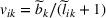
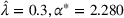
Figure 3 presents the computational results of the 60 COMP instances. Specifically, Figure 3a shows the percentage of instances that are solved optimally (the y‐axis) within a given time (the x‐axis). A point in Figure 3 with coordinates (
) thus indicates that for y% of the instances, t[s] is less than x s. The figure demonstrates that EVF‐CP outperforms the others: The red solid line is consistently above the others, meaning that given the same computational budget, EVF‐CP can solve more instances. In total, 95.0% of the instances can be solved optimally within the time limit using EVF‐CP, followed by EVF‐OA, which solves 83.3% of the instances. By contrast, the performance of VF‐based approaches is not satisfactory. In particular, VF‐OA can only manage to solve 33.3% of the instances. Similarly, Figure 3b depicts the percentage of instances solved within a given rgap with a time limit of 3600 s. A point in the figure with coordinates (
) thus indicates that for y% of the instances, rgap at termination is less than x%. The maximum rgap for EVF‐CP is only 0.33%, showing that all instances are solved within a small relative gap. Besides that, the EVF‐based approaches dominate the VF‐based approaches as we can observe major differences between them in Figure 3b.
Computational results of the 60 COMP instances under FEF
Through the above discussion, we can conclude that the proposed Algorithm 2 is very effective for BCFL‐VM under FEF. In particular, EVF‐CP is substantially more efficient than the VF‐based approaches. Thus, we recommend EVF‐CP as a primary methodology to solve such a problem.
Result analysis under EEF
We now proceed to the analysis of the results under EEF. Without loss of generality, we set
,
, that is, the elasticity parameter is identical for all customer zones. Note that under EEF (except that of the special case where
), only EVF‐OA is applicable. Therefore, we only test EVF‐OA here.
CFLDP results
Table 2 reports the computational results of the CFLDP instances. Here, we use MS[%] to denote the market size, computed by the summation of the leader's objective and the follower's objective and then divided by the maximum possible market size, that is,
. According to the table, the performance of EVF‐OA is impressive because all instances can be solved optimally, and the maximum computational time is only 416 s. However, compared to the FEF instances, the number of iterations seems to be more unstable. It turns out that #Itr can go up to more than 24. Nevertheless, thanks to the convexity and powerfulness of the proposed framework, it is indeed not computationally expensive to solve both MP(Υ) and FSP(
). Therefore, despite requiring a large number of iterations for some instances, the algorithm is still rather efficient.
Results of the 42 CFLDP instances under EEF
t[s]
#Itr
Π
Φ
MS[%]
t[s]
#Itr
Π
Φ
MS[%]
t[s]
#Itr
Π
Φ
MS[%]
20
40
2.9
1
30.8
67.0
38.5
6.4
2
45.3
97.9
56.4
4.0
1
64.9
132.0
77.5
30
60
10.1
3
39.0
91.8
51.5
9.9
3
54.6
122.7
69.8
18.7
4
72.0
153.3
88.7
30
70
6.4
2
38.5
99.8
54.4
7.1
2
52.5
136.4
74.4
18.2
4
63.9
167.0
90.9
30
90
11.1
3
36.3
118.1
60.8
21.2
3
47.6
156.2
80.2
56.0
5
55.1
184.1
94.2
40
20
1.6
1
67.1
30.7
38.5
1.7
1
97.9
45.3
56.4
2.3
1
131.2
62.3
76.2
40
50
14.9
5
53.9
75.3
50.9
63.4
11
74.7
100.7
69.1
416.0
29
94.9
131.7
89.3
40
80
28.0
4
49.8
102.4
59.9
56.9
4
65.3
136.8
79.6
71.4
5
76.3
161.9
93.8
40
90
91.5
9
47.4
114.0
63.5
59.7
4
62.7
145.7
82.0
53.2
4
72.2
169.5
95.2
50
40
16.5
5
73.7
53.8
50.2
13.0
4
103.3
76.7
70.9
4.9
1
130.6
97.8
89.9
60
30
2.3
1
91.8
39.0
51.5
19.2
6
124.3
53.9
70.2
2.9
1
157.3
71.1
89.9
70
30
12.1
4
99.8
38.5
54.4
3.1
1
137.7
51.2
74.4
5.8
1
164.8
66.1
90.9
80
40
358.3
24
103.4
46.8
59.1
25.6
2
141.2
63.5
80.6
307.5
7
163.1
77.8
94.8
90
30
61.9
10
118.1
36.3
60.8
11.0
1
158.4
46.3
80.6
18.9
1
181.6
57.2
94.0
90
40
107.3
9
111.9
48.0
63.0
54.4
3
149.3
59.8
82.3
315.3
4
170.9
71.1
95.3
COMP results
We then look at the COMP instances. Here, we use four structured problem data (i.e., 111w, 211w, 311w, and 411w). For each data, we consider
and
. The number of instances are 64. The results are reported in Table 3 where each row shows the summary statistics of the four structured problem data.
and
are the average leader's objective and market size.
Results of the 64 COMP instances under EEF using EVF‐OA
t[s]
rgap[%]
#Itr
λ
B
Avg
Max
Avg
Max
Avg
Max
0.1
3
1.6
1.7
0
0
1.0
1
670.4
14.6
5
1.8
2.1
0
0
1.0
1
1036.6
22.4
7
5.2
10.5
0
0
2.0
3
1362.6
29.2
10
3.0
5.8
0
0
1.4
3
1780.1
38.0
0.3
3
5.4
11.4
0
0
1.8
3
1618.5
34.7
5
60.5
155.5
0
0
5.8
11
2330.0
49.8
7
332.7
1208.8
0
0
8.3
26
2873.0
61.2
10
1080.4
2582.7
0
0
16.0
36
3446.6
73.2
0.5
3
26.8
83.7
0
0
4.3
11
2268.1
48.7
5
938.2
1515.3
0
0
19.5
29
3096.3
65.8
7
1575.4
3600.0
0.25
0.98
8.5
16
3634.8
77.0
10
1970.1
3600.0
0.60
1.56
4.3
11
4111.1
87.1
∞
3
4.0
6.9
0
0
1.3
2
4755.7
100.0
5
9.9
11.0
0
0
1.5
2
4734.4
100.0
7
21.7
31.7
0
0
1.5
2
4729.5
100.0
10
39.6
74.8
0
0
2.0
2
4736.9
100.0
We observe that the computational difficulty changes with λ: When λ is relatively small (i.e.,
and the demand is extremely elastic) or large (i.e.,
and the demand is inelastic), the instances are easy to handle and require limited iterations (the maximum #Itr is only 3). However, the instances become challenging when the demand elasticity is at medium levels (
and
). Despite that, the EVF‐OA still remains effective: when
, all instances are solved within 1 h; when
, except for the instances under
, we can reach an rgap that is less than 1% upon termination.
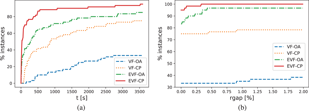
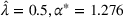
In fact, although some instances are not solved to their optimality within the time limit, the optimal solutions could have been found. This statement is based on the observation that, nearly for all instances, LB quickly grows to the true optimal value of the leader's objective in only a few iterations, and thus most of the computational budget is consumed on reducing UB to prove the optimality of the solution. Figure 4 shows the convergence curves of two instances that require a large number of iterations. It is clear that LB levels off starting from iteration 2‐3, and the large #Itr is owing to the slow movement of UB. In other words, the proposed Algorithm 2 provides an effective framework to generate an optimal leader solution. Therefore, despite the existence of exit gaps for some instances, it is reasonable to believe that high‐quality (even optimal) solutions have been found.
The convergence curves of two 111w instances that require a large number of iterations under EEF
In summary, through the previous computational tests, we conclude that the EVF‐OA is indeed effective to solve BCFL‐VM under EEF.
Table 1 and Table 3 reveal that the EVF‐based algorithms are extremely powerful to solve the instances with inelastic demand (i.e.,
and
). Actually, we have verified its efficiency on a larger scale data set and deferred the numerical results to Supporting Information EC.5.2.
MANAGERIAL IMPLICATIONS
This section conducts experiments to investigate the properties of the BCFL‐VM model and draw insightful observations. Throughout this section, the discussion is conducted on the CFLDP data set.
Win–win scenario
This subsection intends to elaborate on the adaptivity of optimal decisions to the changing business environments. In fact, Table 2 has presented that when one company unilaterally raises the budget, both companies may increase the revenue simultaneously. For example, under
and
, if the leader's budget
increases from 80 to 90, the leader's objective will increase from 103.4 to 119.9, and the follower's objective will increase from 46.8 to 48.0. Therefore, under the bilevel market expansion effect, it is possible that both companies can benefit from the one‐side raising budget activity. We refer to this phenomenon as a win–win scenario.
We now investigate how the win–win scenario occurs using the CFLDP data set under EEF. Based on “who raises the budget,” we classify the win–win scenarios into two types: Type I win–win, in which a win–win scenario happens when the leader raises the budget, and Type II win–win, in which a win–win scenario occurs as the follower raises the budget. By contrast, if the win–win scenario does not occur, that is, the revenue of the company that raises the budget increases but the competitor's decreases, we define such a scenario as raiser dominates, or win–lose (Zhang & Swaminathan, 2020).
We further present the competitive revenue changing details of different scenarios under
in Figure 5. In total, there are 180 unilateral budget‐raising cases (i.e., 180 arrows in the figure). Among them, we have identified six Type I win–win scenarios and five Type II win–win scenarios, indicating that the win–win scenario occurs at a probability of approximately 6%. In addition, we have the following detailed findings.
The Type I win–win occurs mainly when the follower's budget is at a low level (left side of the figure), while the Type II win–win occurs mainly when the leader's budget is at a low level (lower side of the figure). This observation states that when one company does not invest a lot in the market and only opens a small number of facilities, the unilateral budget‐raising activity of the other company will have a small cannibalization effect on its revenue and, to some extent, even lead to improvement in its revenue due to the overall market expansion effect. In other words, given a low budget level, the unilateral action will allow both companies to cannibalize customers from the outside options in the expanded market. The spillover effect is then more likely to dominate the cannibalization effect, thereby leading to the win–win outcomes.
When both the leader's and the follower's budgets are at high levels, the win–win scenarios rarely happen (i.e., all arrows in the upper right corner of the figure are blue). The reason can be traced back to the concavity of the market size function. If both companies set large budgets to offer services, the customers have already perceived high utilities. Given this, the market size has been developed to a rather high level, and the marginal incremental of market size induced by raising budget will be insignificant according to the concavity of the EEF. Consequently, the unilateral action will make the cannibalization effect dominate the spillover effect and, thus, the budget‐raising company will cannibalize customers from the rival in the almost unchanged market.
“Win–win” and “Raiser dominates” scenarios under
. The numbers in the parenthesis
indicate that the leader's budget is x and the follower's budget is y
The above findings suggest that win–win scenarios are more likely to happen in a market where there are imbalanced budgets (positions) between two competing companies (e.g., a large and a small company). Essentially, this result reflects the revenue trade‐off between cannibalization and spillover effects caused by raising budgets. Generally, when the spillover effect is significant, we have more chances to witness the win–win outcome, and vice versa. In the extreme case where the market size is fixed, a win–win scenario will never occur as the “gain” of one company means the cannibalized “loss” of the other.
Note that the significance of the spillover effect is also affected by the parameter λ. If λ is higher, then the market size shows lower elasticity, and win–win scenarios are expected to happen less often. Table 4 reports all win–win scenarios under one‐side budget expansion. We can observe that the number of win–win scenarios clearly decreases with λ. In particular, only one scenario is observed when
.
Seventeen win–win scenarios under one‐side budget raising
Type
λ
I
0.5
(10,10)
→
(20,10)
(17.9,17.9)
→
(33.5,18.5)
0.5
(50,20)
→
(60,20)
(83.5,26.2)
→
(92.4,27.2)
0.5
(60,10)
→
(70,10)
(98.1,14.0)
→
(107.3,14.6)
0.5
(80,40)
→
(90,40)
(103.4,46.8)
→
(111.9,48.0)
0.5
(90,10)
→
(100,10)
(126.2,12.6)
→
(134.1,13.5)
0.5
(90,20)
→
(100,20)
(122.3,22.3)
→
(130.4,24.0)
1.0
(50,20)
→
(60,20)
(117.1,38.5)
→
(126.1,39.5)
1.0
(60,10)
→
(70,10)
(138.2,20.9)
→
(151.4,21.3)
1.0
(80,20)
→
(90,20)
(156.1,34.1)
→
(163.7,34.5)
2.0
(80,20)
→
(90,20)
(190.2,41.4)
→
(191.7,44.2)
II
0.5
(10,10)
→
(10,20)
(17.9,17.9)
→
(18.5,33.5)
0.5
(10,60)
→
(10,70)
(14.0,98.1)
→
(14.6,117.2)
0.5
(10,90)
→
(10,100)
(12.6,126.2)
→
(13.5,134.1)
0.5
(20,60)
→
(20,70)
(24.9,94.6)
→
(26.1,104.7)
0.5
(50,90)
→
(50,100)
(59.1,106.8)
→
(59.3,111.3)
1.0
(10,60)
→
(10,70)
(20.9,138.2)
→
(21.3,151.4)
1.0
(20,90)
→
(20,100)
(30.9,164.5)
→
(31.2,172.3)
Opportunity revenue loss of market size function
We now discuss the choice of market size function and its impact on the leader's revenue loss to shed light on the value of unifying two types of market size functions into an integrated modeling framework. This is a key concern for the decision maker as the market size function is a fundamental input for the BCFL‐VM model. To address the concern, we assume that the leader is provided with real data points about the market size and utility from marketing department. Moreover, the leader is facing two possible choices, FEF and EEF, but she is not sure which one is true when only relying on the given data set. Therefore, she has to gamble by choosing one type of function according to her experience, either FEF or EEF, estimating the relevant parameters from the data, and then adopting the selected function for the BCFL‐VM model. If the leader's choice is correct, the company will not incur revenue loss; otherwise, a revenue loss may arise due to her fault.
Obviously, there are four possible combinations between the true market size function and the leader's choice: (FEF, FEF), (FEF, EEF), (EEF, FEF), and (EEF, EEF), where the first element in each bracket pair represents the true market size function and the second element indicates the leader's choice. Among the four pairs, only the scenarios (FEF, EEF) and (EEF, FEF) would lead to leader's revenue loss as she has chosen the wrong function, whose loss will be analyzed in this subsection.
Scenario (FEF, EEF)
The true market size function follows FEF but the leader chooses to use EEF. Thus, EEF is going to be estimated with a few data points sampled from the true function FEF. Note that both market size functions only have one distinct parameter: α for FEF in (36) and λ for EEF. Therefore, given a true value of
, we can sample a set of data points following FEF and then estimate the value of
for EEF with the generated data set. For conciseness, we discuss the details of sampling data points and estimating parameters in Supporting Information EC.7. Moreover, we denote the leader's revenue obtained by solving BCFL‐VM under the true market size function as optimal revenue Π. Similarly, we denote that revenue under the estimated market size function as estimated revenue
and the leader's solution as
. Given
, we solve FSP(
) under FEF to derive the actual response of the follower
. Then, the actual revenue of the leader
can be evaluated based on the solution
under FEF. Therefore, the opportunity revenue loss is defined as
, which reflects the relative loss of revenue caused by an incorrect choice of the leader.
Given the case (FEF, EEF), Table 5 reveals the opportunity revenue loss under different
values and the corresponding estimated
values. We have the following observations from the table: (i) Revenue loss indeed exists due to the incorrect choice of market size function and, for some instances, such a loss can be substantial. The maximum Δ reaches 9.24%, indicating that when EEF is mistakenly adopted, the decision could significantly deviate from that employing the correct FEF. (ii) On average, such deviation becomes more significant (
) as the demand elasticity increases. Moreover, the revenue estimation error
also increases in
, which can be explained by the error of the market size function estimation as shown in Supporting Information EC.7; that is, the error shows a positive relationship with the demand elasticity. (iii) Surprisingly, the revenue estimation error will be rather significant for certain cases. For example, given
, the average values of
and Π are 33.0 and 43.8, respectively, indicating that the leader underestimates the revenue by as much as 24.66%. Consequently, if the leader misinterpreted the true market size function FEF as EFF, the decisions would be overconservative when planning the budget level required for facility open and decoration decisions in the initial stage, thereby dampening the company's incentive to invest on expansion.
The leader's revenue and opportunity loss under the scenario (FEF, EEF)
Π
Π
Π
Π
20
40
53.7
55.6
55.6
0
36.9
45.3
45.3
0
20.0
26.4
26.4
0
14.7
19.9
19.9
0
30
60
61.7
62.2
62.2
0
46.2
51.4
51.4
0
25.4
32.8
32.9
0.30
19.3
25.2
25.2
0
30
70
58.7
57.2
57.2
0
45.4
48.9
48.9
0
24.8
32.2
32.2
0
18.3
24.7
24.7
0
30
90
52.1
49.8
49.8
0
42.0
43.5
43.5
0
23.6
28.5
30.0
5.00
18.0
21.8
22.6
3.54
40
20
114.5
121.9
121.9
0
81.5
97.4
97.4
0
41.5
58.2
58.2
0
30.1
42.8
42.8
0
40
50
84.8
84.7
85.5
0.94
63.5
64.8
71.4
9.24
34.8
45.7
45.7
0
26.0
34.8
34.8
0
40
80
71.5
68.4
68.4
0
57.6
59.8
59.8
0
32.4
41.4
41.4
0
25.2
31.5
31.5
0
40
90
68.1
64.7
64.7
0
55.9
57.1
57.1
0
31.9
38.7
39.3
1.53
25.0
30.6
30.6
0
50
40
121.4
113.1
116.1
2.58
87.2
96.2
96.3
0.10
47.7
62.0
62.0
0
35.4
46.9
47.4
1.05
60
30
143.9
139.9
140.9
0.71
107.8
117.2
118.7
1.26
56.6
72.3
76.8
5.86
41.3
55.3
56.1
1.43
70
30
152.5
147.9
147.9
0
118.5
125.5
127.6
1.65
64.9
82.2
83.8
1.91
45.5
58.5
63.5
7.87
80
40
153.5
145.9
146.0
0.07
120.9
124.6
128.4
2.96
68.6
85.5
86.0
0.58
51.1
66.5
67.2
1.04
90
30
172.5
163.9
163.9
0
140.7
144.1
144.1
0
75.6
93.6
97.3
3.80
56.2
70.4
74.8
5.88
90
40
162.4
151.0
152.8
1.18
129.9
129.0
135.3
4.66
75.3
92.8
92.8
0
56.3
71.9
72.7
1.10
Average
105.1
101.9
102.4
0.47
81.0
86.1
87.5
1.67
44.5
56.6
57.5
1.55
33.0
42.9
43.8
2.12
Scenario (EEF, FEF)
The true market size function follows EEF but the leader chooses FEF. The leader will estimate
given true
to obtain the estimated FEF for the BCFL‐VM model (also see Supporting Information EC.7). Table 6 reports the revenue and opportunity loss under different
and corresponding estimated
. We conclude similar findings as the previous scenario: The maximum loss Δ can reach 6.35% when
and
. Besides, Δ increases as
decreases, showing that the opportunity loss becomes larger when customers' demand is more elastic. In addition, the revenue estimation error could also be significant. Specifically, under
, the average values
and Π are 65.0 and 51.4, respectively, given which, the revenue is overestimated by 26.46%. Therefore, if the leader misinterpreted the true market size functions EEF as FEF, the decisions would be over aggressive when determining the expansion plan, thereby amplifying the investment risk.
The leader's revenue and opportunity loss under the scenario (EEF, FEF)
Π
Π
Π
Π
20
40
13.5
10.4
10.4
0
30.4
23.1
23.1
0
40.8
29.7
30.8
3.57
52.5
45.3
45.3
0
30
60
17.6
14.3
14.3
0
37.5
29.1
29.1
0
47.4
39.0
39.0
0
59.3
53.1
54.6
2.75
30
70
16.8
13.1
13.9
5.76
36.5
28.6
28.6
0
45.4
38.5
38.5
0
55.1
52.5
52.5
0
30
90
16.2
13.9
13.9
0
33.6
25.6
26.5
3.40
40.8
36.3
36.3
0
48.3
47.6
47.6
0
40
20
28.3
21.3
21.3
0
67.6
48.5
48.5
0
88.3
67.1
67.1
0
115.4
97.9
97.9
0
40
50
23.9
18.9
18.9
0
52.1
40.1
40.1
0
65.8
53.8
53.9
0.19
81.9
74.7
74.7
0
40
80
22.2
18.5
18.5
0
46.3
36.9
36.9
0
56.1
49.8
49.8
0
66.3
65.3
65.3
0
40
90
21.9
18.4
18.4
0
43.2
33.9
36.2
6.35
53.7
46.5
47.4
1.90
62.8
62.7
62.7
0
50
40
32.8
25.1
25.5
1.57
70.6
54.5
55.2
1.27
88.8
73.1
73.7
0.81
111.7
101.7
103.3
1.55
60
30
38.6
29.8
30.3
1.65
87.0
65.1
65.4
0.46
108.6
91.8
91.8
0
135.7
124.3
124.3
0
70
30
42.5
33.3
34.3
2.92
95.0
70.9
75.0
5.47
119.1
97.6
99.8
2.20
142.9
137.7
137.7
0
80
40
46.3
36.7
38.3
4.18
96.0
78.8
78.8
0
120.7
103.4
103.4
0
141.7
140.7
141.2
0.35
90
30
51.2
41.1
42.4
3.07
109.9
86.0
89.4
3.80
135.4
114.8
118.1
2.79
158.3
157.4
158.4
0.63
90
40
50.9
40.7
42.1
3.33
103.7
86.3
86.3
0
126.6
110.5
111.9
1.25
148.5
149.3
149.3
0
Average
30.2
24.0
24.5
2.04
65.0
50.5
51.4
1.63
81.3
68.0
68.7
1.00
98.6
93.6
93.9
0.35
To summarize, if an inappropriate market size function is selected for the BCFL‐VM problem, it is risky to incur substantial revenue loss. Meanwhile, the company may be misled to overaggressiveness/conservativeness in its expansion plan and may put itself in a dilemma. In practice, the market size function is going to be estimated from industrial/business data. It is, of course, not possible to find a type of function that perfectly fits all scenarios given different business environment, but it is indeed meaningful to provide alternatives in response to various practical applications. Our methodology exactly unifies two types of market size functions into an integrated framework, allowing the company to select the one that yields a better estimation performance, thereby boosting the chance to achieve optimal decisions and reducing the risk/magnitude of revenue loss.
DISCUSSION AND CONCLUSION
We studied a BCFL‐VM where two companies (a leader and a follower) open and design facilities sequentially to maximize their own revenue. The total market size is elastic and depends on the utility jointly provided by the leader's and the follower's facilities. Given the facilities, customers determine which one to patronize following the proportional choice rule. The problem is to search for the best location and design strategy for the leader upon anticipating the follower's reaction. We formulated the problem as a nonlinear 0‐1 bilevel program. To date, there exists no exact algorithm for BCFL‐VM. Motivated by this gap, we proposed two exact frameworks. The first one is based on the value‐function–based approach, where we first restated the bilevel model into a single‐level model and then developed an iterative algorithm that alternates between an upper bounding problem and a lower bounding problem. However, the upper bounding problem is in general nonconvex, which causes a significant inefficiency in the framework. To avoid handling such a complicated problem, we proposed a new bounding problem that possesses a convex structure. We then designed general and customized approaches to solve both bounding problems. Through extensive computational studies, we demonstrated that the solution approaches are effective in addressing BCFL‐VM. In particular, our proposed algorithm can tackle instances with hundreds of location variables.
By leveraging the design parameters in computational tests, our research leads to several important insights for (chained) business management. First of all, we know that if either company (leader or follower) raises the budget level, intuitively, the overall market size would get expanded such that both companies will benefit from a larger market size. However, numerical tests show that such a “win–win” outcome rarely happens. On the contrary, it is rather common to observe that the budget‐raising company indeed not only acquires additional new market size but also slightly cannibalizes the original market size from the competitor. We intend to provide a reasonable explanation for this phenomenon: When the leader and follower are in imbalanced positions (i.e., a large and a small company, respectively), raising the budget has more opportunities to reach the win–win outcome as the spillover effect would dominate the cannibalization effect in the expanded market. By contrast, if both companies are in similar positions, the budget‐raising action would cause the cannibalization effect over the spillover effect, thereby resulting in the “raiser dominates” consequence. If so, the leader's manager should squeeze the potential budget improvement space of the follower when they make the initial decisions. Moreover, depending on the different types of market size function, the optimal decisions seem more challenging to achieve under EEF than FEF as the FEF‐based model can possibly be reformulated into a model with the standard proportional rule (see Supporting Information EC.5.1). Therefore, in practice, if both EEF and FEF present similar fitting performance on real data sets, then we recommend managers to adopt FEF for customer preference description as it shows better computationally adaptivity. However, if both functions exhibit different fitting behaviors, then we also show that the misapplication of the market size function would result in substantial revenue loss and may further mislead the expansion plan in an overaggressive/conservative way. Finally, apart from the location and design decisions, our proposed approaches are easily generalizable to address broader choice‐set decisions. For example, regarding decisions on new product development, in 2015, Apple Inc. first introduced the Apple Watch into the wearable devices market and it quickly became the best selling product of the year (Paul, 2016). Witnessing the success, several months later, other companies such as Samsung and Huawei immediately joined this competition and unveiled their own wearable products to capture the growing market share. By defining the utility appropriately, for example, incorporating the features of product design, quality, and price, our approach can support the leader company (i.e., Apple) in acquiring more revenue when launching new products with certain advanced demand information.
There are also limitations and potential future directions regarding the current work. We assumed that customers follow the proportional choice rule. Although the usage of such a rule is prevailing, it is often argued that not all facilities will be considered by customers. In other words, given a set of open facilities, customers will only show interest in a subset of the open facilities. They form a “consideration set” subject to certain conditions. Only facilities in the set will be chosen with positive probability. We point out that when customers are forming the consideration set, there might be an embedded optimization problem. BCFL‐VM may then become a trilevel model, where the leader makes the location decision in the first level, the follower reacts accordingly in the second level, and customers form the consideration set and select which facility to visit in the third level. Naturally, the trilevel problem is extremely challenging, and we would like to leave this aspect for future research.
Footnotes
ACKNOWLEDGMENTS
The authors thank the departmental editor, senior editor, and two anonymous reviewers for their helpful and constructive comments that helped improve this paper significantly.
AboolianR.BermanO.KrassD. (2007). Competitive facility location model with concave demand. European Journal of Operational Research, 181(2), 598–619.
2.
AdjimanC. S.AndroulakisI. P.FloudasC. A. (2000). Global optimization of mixed‐integer nonlinear problems. AIChE Journal, 46(9), 1769–1797.
3.
AlekseevaE.KochetovY.PlyasunovA. (2015). An exact method for the discrete ‐centroid problem. Journal of Global Optimization, 63(3), 445–460.
4.
BalochG.GzaraF. (2020). Strategic network design for parcel delivery with drones under competition. Transportation Science, 54(1), 204–228.
5.
BeresnevV. (2013). Branch‐and‐bound algorithm for a competitive facility location problem. Computers & Operations Research, 40(8), 2062–2070.
6.
BeresnevV.MelnikovA. (2018). Exact method for the capacitated competitive facility location problem. Computers & Operations Research, 95(6), 73–82.
7.
BermanO.DreznerT.DreznerZ.KrassD. (2009). Modeling competitive facility location problems: New approaches and results. In OskoorouchiM. R.GrayP. (Eds.), Decision technologies and applications (pp. 156–181). INFORMS.
8.
BiesingerB.HuB.RaidlG. (2015). A hybrid genetic algorithm with solution archive for the discrete ‐centroid problem. Journal of Heuristics, 21(3), 391–431.
9.
BiesingerB.HuB.RaidlG. (2016). Models and algorithms for competitive facility location problems with different customer behavior. Annals of Mathematics and Artificial Intelligence, 76(1‐2), 93–119.
10.
CostHack (2021). How much does Nike franchise costs?https://costhack.com/nike‐franchise‐cost/
11.
DownsA. (1957). An economic theory of democracy. New York: Harper.
12.
DreznerT. (2006). Derived attractiveness of shopping malls. IMA Journal of Management Mathematics, 17(4), 349–358.
13.
DreznerT.DreznerZ. (2017). Leader‐follower models in facility location. In PardalosP.ThaiM. T. (Eds.), Spatial interaction models (pp. 73–104). Springer.
14.
DreznerT.DreznerZ.KalczynskiP. (2015). A leader–follower model for discrete competitive facility location. Computers & Operations Research, 64, 51–59.
15.
EmmaT. (2019). Nike town: On the road. https://www.pivotalretailmarketing.co.uk/index.php/2019/07/04/nike‐town‐on‐the‐road/
16.
FischettiM.LjubićI.MonaciM.SinnlM. (2017). A new general‐purpose algorithm for mixed‐integer bilevel linear programs. Operations Research, 65(6), 1615–1637.
17.
FreireA. S.MorenoE.YushimitoW. F. (2016). A branch‐and‐bound algorithm for the maximum capture problem with random utilities. European Journal of Operational Research, 252(1), 204–212.
18.
GentileJ.PessoaA. A.PossM.RoboredoM. C. (2018). Integer programming formulations for three sequential discrete competitive location problems with foresight. European Journal of Operational Research, 265(3), 872–881.
19.
KleinertT.LabbéM.LjubićI.SchmidtM. (2021). A survey on mixed‐integer programming techniques in bilevel optimization. EURO Journal on Computational Optimization, 9, 100007.
20.
KleniatiP. M.AdjimanC. S. (2015). A generalization of the branch‐and‐sandwich algorithm: From continuous to mixed‐integer nonlinear bilevel problems. Computers & Chemical Engineering, 72, 373–386.
21.
KochetovY.KochetovaN.PlyasunovA. (2013). A matheuristic for the leader‐follower facility location and design problem. In Proceedings of the 10th metaheuristics international conference (MIC 2013) (Vol. 32, p. 3). Citeseer.
22.
KüçükaydinH.ArasN.AltınelI. K. (2011). Competitive facility location problem with attractiveness adjustment of the follower: A bilevel programming model and its solution. European Journal of Operational Research, 208(3), 206–220.
23.
LinY.TianQ. (2021a). Exact approaches for competitive facility location with discrete attractiveness. Optimization Letters, 15(2), 377–389.
24.
LinY. H.TianQ. (2021b). Branch‐and‐cut approach based on generalized benders decomposition for facility location with limited choice rule. European Journal of Operational Research, 293(1), 109–119.
25.
LinY. H.TianQ. (2021c). Generalized benders decomposition for competitive facility location with concave demand and zone‐specialized variable attractiveness. Computers & Operations Research, 130, 105236.
26.
LjubićI.MorenoE. (2018). Outer approximation and submodular cuts for maximum capture facility location problems with random utilities. European Journal of Operational Research, 266(1), 46–56.
27.
LozanoL.SmithJ. C. (2017). A value‐function‐based exact approach for the bilevel mixed‐integer programming problem. Operations Research, 65(3), 768–786.
28.
LuceR. D. (2012). Individual choice behavior: A theoretical analysis. Courier Corporation.
29.
LyuG.TeoC. P. (2022). Last mile innovation: The case of the locker alliance network. Manufacturing & Service Operations Management, Forthcoming.
30.
MallozziL.D'AmatoE.PardalosP. M. (2017). Spatial interaction models. Springer.
31.
MitsosA. (2010). Global solution of nonlinear mixed‐integer bilevel programs. Journal of Global Optimization, 47(4), 557–582.
32.
PaulL. (2016). Apple watch sales hit 12 million in 2015. https://www.wareable.com/smartwatches/apple‐watch‐sales‐hit‐12‐million‐in‐2015‐2279
33.
Statista. (2021). Number of retail stores of the Adidas group worldwide from 2008 to 2020, by store type. https://www.statista.com/statistics/268442/
34.
SuharaY.BahramiM.BozkayaB.PentlandA. S. (2021). Validating gravity‐based market share models using large‐scale transactional data. Big Data, 9(3), 188–202.
35.
TahernejadS.RalphsT.DeNegreS. (2020). A branch‐and‐cut algorithm for mixed integer bilevel linear optimization problems and its implementation. Mathematical Programming Computation, 12(4), 529–568.
36.
TiwariR.JayaswalS.SinhaA. (2021). Alternate solution approaches for competitive hub location problems. European Journal of Operational Research, 290(1), 68–80.
37.
WangR. (2021). Consumer choice and market expansion: Modeling, optimization, and estimation. Operations Research, 69(4), 1044–1056.
38.
WuD.LuoC.WangH.BirgeJ. R. (2016). Bi‐level programing merger evaluation and application to banking operations. Production and Operations Management, 25(3), 498–515.
39.
XiongJ.WangS.NgT. S. (2021). Robust bilevel resource recovery planning. Production and Operations Management, 30(9), 2962–2992.
40.
YeJ. J. (2006). Constraint qualifications and KKT conditions for bilevel programming problems. Mathematics of Operations Research, 31(4), 811–824.
41.
ZhangY.SwaminathanJ. M. (2020). Warehouse location in an emerging country: A win–win proposition?Production and Operations Management, 29(6), 1487–1505.