Fulfillment scheduling for buy‐online‐pickup‐in‐store orders

Abstract

One of the most popular ways of shopping in an omnichannel retailing environment is buy‐online‐pickup‐in‐store (BOPS). Retailers often promise BOPS shoppers short in‐store pickup ready times. We study fulfillment scheduling decisions of BOPS orders destined for a single store of a retailer. There are two fulfillment options for BOPS orders: they can be either processed at a fulfillment center (FC) and delivered to the store or processed at the store without needing delivery. There are two types of trucks available to deliver the BOPS orders fulfilled at the FC: prescheduled trucks that are already committed to replenishing store inventory and have some spare capacity that can be utilized, and additional trucks that can be hired from third‐party logistics providers. There is a fixed cost for using each truck; the cost for using a prescheduled truck is lower than that for using an additional truck. If an order is fulfilled at the store, it incurs a processing cost and a processing time, whereas the processing cost and time are negligible if an order is fulfilled at the FC. The problem is to determine where to fulfill each order (FC vs. the store), how to assign the orders fulfilled at the FC to trucks for delivery, and how to schedule the orders fulfilled at the store for store processing, so as to minimize the total fulfillment cost, including the delivery cost from the FC to the store incurred by the orders processed at the FC, and the processing cost for fulfilling the rest of the orders at the store, subject to the constraint that each order is ready for pickup at the store by its promised pickup ready time. We consider various cases of the problem by clarifying their computational complexity, developing optimal algorithms and heuristics, and analyzing theoretical performance of the heuristics. We also conduct computational experiments to validate the effectiveness of the proposed heuristics in both static and dynamic settings and derive important insights about how the presence of prescheduled trucks and the presence of store fulfillment option impact the fulfillment cost and decisions.

INTRODUCTION

Recent advances in information technologies such as smartphones, high‐speed Internet, and social media have empowered consumers to use both online and off‐line retail channels to shop and demand a consistently good buying experience across all channels. As a response, a growing number of retailers have adopted or are transitioning to omnichannel retailing (OCR; Bell et al., 2014; Brynjolfsson et al., 2013; Cai & Lo, 2020; Verhoef et al., 2015). OCR seamlessly integrates off‐line and online retailing and provides shoppers with more flexibility and convenience, compared to traditional multichannel retailing in which different channels are often operated in silos. In an OCR environment, a shopper can place an order online from a computer at home, from her cell phone while working at office, or from a kiosk while shopping in a brick‐and‐mortar store, and have the product delivered to her home. The same shopper can also, if she prefers, have her online order delivered to a store or a locker near her home and pick it up later. Whichever ordering and delivery option a customer chooses, OCR is supposed to provide the customer with a cohesive user experience at every touchpoint, including showing the same user‐friendly online interface, displaying the same product availability and pricing information, and offering the same return policy and after‐sales service support.

One of the most popular ways of shopping in an OCR‐enabled environment is buy‐online‐pickup‐in‐store (BOPS; Gallino & Moreno, 2014; Gao & Su, 2017; Song et al., 2020). BOPS allows customers to make an order online and pick up the fulfilled order from a store near their homes, which provides customers with the best of both online and off‐line worlds. On the one hand, they can use the online channel to do research, read reviews, compare prices, make payments, and enjoy the convenience of hassle‐free shopping. On the other hand, they do not need to pay a shipping fee because their orders are not shipped to their homes, and usually wait much less time to get their orders compared to home delivery because the lead time promised by the retailer for store pickup is often much shorter than that for orders delivered to customers’ homes. JDA's 2016 consumer survey shows that 46% of respondents have used BOPS in the 12 months prior to the survey (JDA, 2016). A more recent consumer survey (Cassidy, 2019) shows that 85% of consumers have shopped both online and in a physical store in the 6 months prior to this survey, with 73% of these shoppers using BOPS. Data points linked to some individual retailers show a similar trend. Forty percent of Best Buy's and more than 50% of Walmart's online sales involve in‐store pickups (Evans, 2018; Roose, 2017). From retailers’ point of view, allowing online shoppers to pick up orders in store increases traffic in the store, thus bringing more potential sales (Clifford, 2011; UPS, 2015). Accordingly, a growing number of retailers offer the BOPS option to their customers. Retail Systems Research report that 64% of retailers in the United States have implemented BOPS (Rosenblum & Kilcourse, 2013). A similar percentage of Europe's top 500 retailers offer such an option (Jindal, 2017).

However, retailers that provide BOPS services to their customers are faced with a whole host of new operational challenges and have to make a new set of decisions, including the following, among others:

product offering decisions, for example, which products should be included in the BOPS services?

store decisions, for example, which stores should offer such services?

pricing decisions, for example, should the BOPS products be priced differently from the same products sold through different channels?

inventory decisions, for example, how much inventory should be kept for a BOPS product?

fulfillment decisions, for example, where should the BOPS orders be processed, at the store, at a fulfillment center (FC), or at a dedicated warehouse? How should the BOPS orders be delivered to the store?

A variety of these and related issues have been addressed in several studies that have appeared in recent years. Gao and Su (2017) use a stylized model to investigate what types of products are suitable for BOPS, and how BOPS impacts the store operations. Several studies (e.g., Kong et al., 2020; Lin et al., 2020; Xu et al., 2021) look into pricing decisions and related issues in settings where the BOPS option is available. Some other studies (e.g., Hu et al., 2022; Saha & Bhattacharya, 2020; Xu et al., 2017) investigate inventory‐related decisions in similar settings. There are also papers (e.g., Harsha et al., 2019; Lei et al., 2018) that consider pricing and inventory decisions in other omnichannel or e‐commerce settings where BOPS services may not be available.

In this paper, we study fulfillment scheduling decisions faced by an omnichannel retailer for the BOPS orders destined to a particular store of the retailer, from which the customers who made these orders are going to pick up their orders. The retailer has two fulfillment options available for each BOPS order: Either it is first processed (i.e., picked and packed) at a FC and then delivered to the store, or it is processed directly at the store. Some prescheduled trucks, each with some spare capacity, and an infinite number of additional trucks, each with a full capacity, can be dispatched to deliver the BOPS orders processed at the FC to the store. The retailer needs to determine (i) which BOPS orders are to be fulfilled through the FC and which are fulfilled at the store directly, (ii) how to assign the orders processed at the FC to available trucks for delivery, and (iii) how to schedule the processing operations of the orders fulfilled at the store, so as to minimize the total order fulfillment cost for the BOPS orders. Section 1.1 describes the problem in detail.

Research on order processing and order delivery decisions in omnichannel environments is relatively new. Our review of related literature in Section 2 shows that most existing studies in this area deal with delivery routing and other distribution‐related issues alone, or order picking and scheduling issues alone. None of them have considered the three main issues involved in our problem jointly: fulfillment location issue (i.e., where to fulfill orders, FC vs. the store), scheduling issue (i.e., how to process orders in the store, and how to assign orders to prescheduled trucks which have fixed departure times), and delivery issue (i.e., how to pack and deliver orders from the FC to the store). Mathematically, our problem is also somewhat related to several other classes of problems, including bin packing, knapsack, and machine scheduling. Our literature review in Section 2 shows that our problem differs from these existing problems significantly in several major aspects.

Problem description

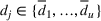
We now describe our problem and introduce the necessary notation. At the beginning of a planning horizon, a retailer has received a set of n BOPS orders N = {1, 2, …, n} destined to a particular store of the retailer, where the orders are picked up by customers. Each order j ∈ N has a size (e.g., weight or volume) of w_j, meaning that it occupies w_j units of capacity when it is loaded into a delivery truck. Retailers almost always promise a certain pickup ready time for a BOPS order. For example, Office Depot, Men's Warehouse, Macy's, and some other retailers promise a pickup ready time of 2 hours from the time of order placement if it is placed certain hours before the store closing time, while CVS, JCPenney, and many others promise same‐day in‐store pickup for orders placed before a certain time of the day (Dwyer, 2020). Thus, in our problem each order j ∈ N has a promised pickup ready time d_j, by which it must be ready at the store for customer pickup. The retailer has two fulfillment options available for each BOPS order:

the order can be first processed at a FC that serves this particular store and then delivered to the store, or

the order can be processed at the store directly, and in this case, no delivery is needed.

Due to the high volume of orders it processes, a FC is often highly automated, has a large order‐processing capacity, and is cost‐efficient. By contrast, a retail store usually has limited space and is not equipped with automated order picking systems. Consequently, order picking and packing operations performed at a store are much more time consuming and much more costly. Thus, it is reasonable to assume that, in our problem, the processing time and cost of any order handled at the FC are negligible, compared to the truck delivery time and cost from the FC to the store and order processing time and cost at the store, and hence are assumed to be 0. However, if an order j ∈ N is fulfilled at the store, then it takes a nonzero processing time p_j and incurs a nonzero processing cost of γ_j for processing the order at the store. Order fulfillment at a store can usually be done sequentially or in parallel. If there are many store personnel dedicated to order fulfillment, then they can be divided into multiple small teams such that multiple orders can be processed in parallel, one at a time by each team. However, if there are few store personnel working on order fulfillment, it is more efficient that they work together to process orders one by one sequentially. We assume that the store in our problem processes the assigned BOPS orders sequentially.

For any BOPS order processed at the store, the fulfillment operation for this order is completed as soon as it is picked and packed. However, for orders processed at the FC, they must be delivered to the store as the last step of the fulfillment operation. The role of FCs is changing due to the ever‐disappearing boundary between online and off‐line retailing. FCs were mainly used to fulfill online orders in the past, but now an increasing number of them may also serve the role of traditional distribution centers so that they handle both business‐to‐business (B2B) and business‐to‐consumer (B2C) orders. In fact, more and more retailers now either convert their existing distribution centers or FCs to hybrid or integrated multifunctional centers, or build such new facilities, to take advantage of inventory and transportation pooling of B2B and B2C orders (Hubner et al., 2016). Urban Outfitters and IKEA are two such examples (Andel, 2014; IKEA, 2018). Thus, we assume that the FC in our problem can not only process BOPS orders but also serve as the source for store inventory replenishment. This means that BOPS orders and store orders can share delivery shipments whenever possible to save transportation cost, which is a part of the total cost considered in our problem.

In practice, retailers often rely on third‐party logistics (3PL) service providers to take care of most of their transportation needs, including those for store inventory replenishment, and for delivery of online orders. Since the inventory of a store has to be replenished on a regular basis, there are delivery trucks going from the FC to the store on a regular basis. Since these trucks are prescheduled and already committed to a given shipment calendar, both their arrival times at the store and their shipment quantities are all known in advance. BOPS orders processed at the FC can get a free ride on these trucks from the FC to the store if these trucks have some spare capacity. We thus assume that in our problem there is a set of prescheduled trucks, each with some spare capacity, going from the FC to the store during the planning horizon that is available to deliver some BOPS orders. No additional transportation cost is incurred by the BOPS orders riding on a prescheduled truck because the truck is going to the store regardless of whether it delivers any BOPS orders or not. However, there is a fixed cost α for using a prescheduled truck to transport some BOPS orders, which represents additional paperwork and loading and unloading operations incurred by the BOPS orders. This fixed cost is expected to be much lower than the transportation cost of the scheduled trip itself.

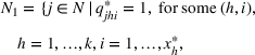
For ease of presentation, we divide the prescheduled trucks in our problem by their arrival times at the store into k subsets, B₁, …, B_k, such that the prescheduled trucks in each subset B_h have the same arrival time at the store τ_h, where without loss of generality it is assumed that τ₁ < τ₂ < ⋅⋅⋅ < τ_k. Let b_h = |B_h| denote the number of prescheduled trucks in B_h, and

$m={\sum }_{h=1}^k{b}_h$

the total number of the prescheduled trucks. Let (h, i) be the index of the ith truck in B_h, where h = 1, …, k and i = 1, …, b_h. Let c_hi denote the spare capacity of prescheduled truck (h, i) that is available to carry orders in N. Without loss of generality, the indices of the prescheduled trucks in each B_h are in a nonincreasing order of their spare capacity, that is, c_h1 ≥ c_h2 ≥ ⋅⋅⋅ ≥

$c_{h,b_h}.$

We say that a prescheduled truck (h₁, i₁) has a smaller index than another prescheduled truck (h₂, i₂) if (h₁, i₁) is lexicographically smaller than (h₂, i₂), that is, h₁ < h₂, or h₁ = h₂ and i₁ < i₂. Furthermore, we assume that the spare capacity of each prescheduled truck c_hi is at least w_max = max _{j ∈N} w_j. Without this assumption, all the results derived in the paper still hold after some minor modifications.

It is unlikely that the prescheduled trucks alone have enough capacity to deliver all the BOPS orders processed at the FC, especially when the BOPS order volume is large. Even if they together do have enough capacity, their scheduled arrival times at the store may be later than the promised pickup ready times of some BOPS orders processed at the FC, and hence they are unable to deliver those orders. Therefore, the retailer may need to use additional trucks to deliver the BOPS orders processed at the FC to the store. Since 3PL providers often have enough reserve transportation capacity to respond to additional service requests, it is reasonable to assume that the retailer in our problem can pay 3PL providers to use as many additional trucks as needed to deliver the BOPS orders that are processed at the FC but are not covered by the prescheduled trucks. Clearly, each additional truck to be used is a dedicated truck for BOPS orders and can depart from the FC at any desired time. Thus, we assume that each additional truck has a full truckload capacity c₀ available, where c₀ > c_hi for any h = 1, …, k and i = 1, …, b_h. Since the processing times of the orders at the FC are assumed to be 0, without loss of generality, we assume that each additional truck used departs from the FC at time 0 and arrives at the store at a time τ₀ that is no later than the arrival time of any prescheduled truck, i.e., τ₀ ≤ τ₁, and no later than any BOPS order's pickup ready time, i.e., d_j ≥ τ₀ for all j ∈ N. It incurs a fixed cost of β if an additional truck is used. This fixed cost includes both the transportation cost from the FC to the store and the order handling cost. Thus, it is reasonable to assume that β > α because α does not include a transportation cost, as discussed earlier. Although the number of additional trucks to be used needs to be determined, for ease of presentation, we let B₀ denote the set of additional trucks used with an unknown number of elements in it initially, and index them as 1, 2, …, such that in any algorithm they are used as needed in this sequence.

Figure 1 illustrates the available trucks that can be used to deliver the BOPS orders processed at the FC to the store. Each vertical bar corresponds to a truck with the available capacity represented by the height of the bar. The trucks are divided into subsets B₀, B₁, …, B_k such that those in each subset have the same arrival time at the store.

FIGURE 1

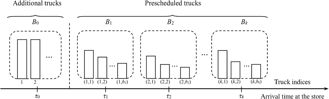
Available trucks with arrival times at the store

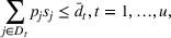
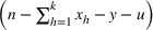
Let u be the number of distinct order pickup ready times, and let these distinct pickup ready times be denoted as

${\overline{d}}_1,\text{…},{\overline{d}}_u$

, where

${\overline{d}}_1<\cdots <{\overline{d}}_u$

. Thus,

$d_j\in \{{\overline{d}}_1,\text{…},{\overline{d}}_u\}$

for j ∈ N. Without loss of generality, we assume that the number of distinct arrival times of the prescheduled trucks at the store (or, simply the number of prescheduled truck sets) k is less than or equal to u. This is because if k > u, then there must exit some h ∈ {1, …, k − 1} such that there is no order j ∈ N with τ_h ≤ d_j < τ_h+1. In this case, we can redefine the arrival time of each truck in B_h at the store to be τ_h+1 and merge the trucks from B_h into B_h+1. This reduces the number of prescheduled truck sets from k to k – 1. We can repeat this process until the number of prescheduled truck sets is reduced to u.

Given the set of BOPS orders N and the various aspects of the fulfillment process, as described above, the retailer needs to determine:

a subset S of the orders in N to be processed at the store (and hence those in

$N\setminus S$

are processed at the FC),

a schedule for processing the orders in S at the store,

a subset X of the prescheduled trucks, and the number of additional trucks, denoted as y, that are used to transport the orders processed at the FC (i.e., those in

$N\setminus S$

), and

a way to assign the orders processed at the FC to the selected trucks,

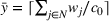
so as to minimize the total fulfillment cost of the BOPS orders, including the total transportation cost of the orders processed at the FC and the total processing cost of the orders processed at the store, that is, F = α|X| + βy +

${\sum }_{j\in S}{\gamma }_j$

, while respecting the truck capacity constraints, the fixed departure times of the prescheduled trucks, and the promised pickup ready times of the orders.

We call this problem fulfillment scheduling problem as the underlying hard constraint of satisfying the promised pickup ready times of the BOPS orders means that scheduling is a critical decision for both order delivery from the FC to the store and order processing at the store. It should be noted that since different orders have different sizes and each truck has a capacity limit, there is a packing decision involved whenever assigning a set of orders to a truck. In addition to the general version of this problem, we also consider a special case where all the BOPS orders are fulfilled through the FC. This special case of the problem involves decisions (iii) and (iv) only. This special case represents settings where stores do not have order fulfillment capability, or even if they have such capability, the retailer decides not to process online orders in stores for the possible negative impact such operations can have on the stores, for example, raising store operational cost, interfering main store operations, and complicating store inventory management, etc. For ease of presentation, we denote the special case as Problem P1 and the general case as Problem P2.

• Problem P1.

Orders in N can only be processed at the FC.

Problem P2.

Orders in N can be processed either at the FC or at the store.

We consider both the splittable case of these problems, denoted as P1S and P2S, respectively, and the nonsplittable case of these problems, denoted as P1N and P2N, respectively. The underlying assumptions associated with each of these problems are as follows:

In problem P1S, an order is allowed to be divided into multiple suborders, each delivered by a separate truck from the FC to the store.

In problem P2S, an order is allowed to be divided into two suborders such that one suborder is fulfilled at the FC and the other at the store, and the suborder fulfilled at the FC is allowed to be divided further into multiple smaller suborders, each delivered by a separate truck to the store, as in problem P1S.

In problem P1N, each order is only allowed to be delivered by one truck from the FC to the store.

In problem P2N, each order is only allowed to be fulfilled at one place, the FC or the store, and each order fulfilled at the FC is only allowed to be delivered by one truck, as in problem P1N.

In the case of P1S and P2S, we allow any possible ways of dividing an order j, as long as the total size of the resulting suborders is equal to w_j. For P2S, if a suborder of order j with size v_j (v_j < w_j) is fulfilled at the store, then the required processing time of this suborder at the store is proportional to its size, i.e.,

$p_j{v}_j/w_j,$

and the processing cost incurred is also proportional to the size, i.e.,

${\gamma }_j{v}_j/w_j.$

Without loss of generality, we assume that parameters w_j and p_j satisfy that p_j = ϕ_jw_j, where ϕ_j is an integer, for j ∈ N. This is a reasonable assumption because p_j and w_j measure different dimensions of an order (i.e., time and size, respectively), we can always properly scale the unit of time while fixing that of order size to achieve the above condition. We note that under this assumption, the processing time of any suborder of order j ∈ N with integer size v_j (v_j ≤ w_j) at the store (i.e.,

$p_j{v}_j/w_j$

) is also an integer. As shown later, for P1S, there exists an optimal solution such that if an order is divided, it is divided into at most two suborders and delivered by two trucks. For P2S, there exists an optimal solution such that if an order is divided, it is divided into at most three suborders with one processed at the store and the other two fulfilled at the FC and delivered by two trucks.

We observe that both problems P1N and P2N are strongly NP‐hard because they contain the strongly NP‐hard bin packing problem (Garey & Johnson, 1979) as a special case. As we show in Section 4, from a theoretical point of view, these problems are much more difficult than the bin packing problem.

Contributions and organization of the paper

We make the following contributions. First, the problem studied is new and motivated by the most recent OCR practices. Hence, our research will inspire more research in this area. Second, we clarify the computational complexity of most cases of the problem, develop exact algorithms and efficient heuristics, and analyze their worst‐case and asymptotic performances. Third, we conduct computational tests to evaluate the performance of the heuristics and derive important managerial insights about BOPS order fulfillment.

The remainder of this paper is organized as follows. In Section 2, we review related literature. In Section 3, we provide some preliminary results to be used in later sections. In Sections 4 and 5, we derive a number of theoretical results, as follows:

In Section 4, we show that (1) problem P1S can be solved in polynomial time, and (2) there is no polynomial time algorithm for problem P1N with a constant worst‐case performance ratio unless P = NP. Furthermore, we develop a fast heuristic H1 for problem P1N and show that its worst‐case performance ratio is bounded by 1 + β/α, and its asymptotic worst‐case performance ratio is bounded by 2.

In Section 5, we show that (1) problem P2S with a fixed number of distinct prescheduled truck arrival times at the stores (i.e., fixed k) can be solved in polynomial time, and (2) problem P2S with a general k is at most ordinarily NP‐hard by giving a pseudo‐polynomial time algorithm. The exact complexity of this problem remains open. In addition, we develop two heuristics H2 and H3 for problem P2N, one for the case with a fixed k, and the other for the case with a general k, and show that their worst‐case performance ratios are bounded by 1 + β (u + 1)/α and 1 + β/α, respectively, and their asymptotic worst‐case performance ratios are both bounded by 2.

In Section 6, we conduct computational experiments. We show that these heuristics perform well, particularly on large‐scale test instances, and derive several important managerial insights about several key elements of the BOPS fulfillment operations. We also demonstrate the effectiveness of applying our heuristics in a rolling horizon fashion to solve a dynamic version of the problems with random order arrivals. Finally, we conclude the paper and discuss several extensions in Section 7. The proofs of all the lemmas and theorems are given in Appendix A1 (Supporting Information), and the technical details for solving the extensions are provided in Appendices A3–A6 (Supporting Information).

LITERATURE REVIEW

In this section, we review the literature on four classes of problems that are related to the problems studied in this paper: order processing and order delivery problems in e‐commerce and OCR, bin packing and knapsack problems, and machine scheduling problems.

Fulfillment operations in e‐commerce and OCR

In recent years, the literature on order fulfillment in the context of e‐commerce and OCR has been growing rapidly. The main issues studied include the trade‐offs between the shipping cost and product availability in different warehouses, and economies of scale resulting from order consolidation, among others. For example, Xu et al. (2009) study the problem of assigning online orders among multiple warehouses and/or drop‐shippers. Acimovic and Graves (2015), and Jasin and Sinha (2015) extend the model of Xu et al. (2009) by considering multiple warehouses, multiple customer locations, and distance‐dependent shipping costs, and develop new near‐optimal fulfillment heuristics. In an OCR setting, Bayram and Cesaret (2020) study order fulfillment decisions under ship‐from‐store business mode. Wei et al. (2021) investigate the benefits of consolidating current orders with future ones. However, none of these papers address detailed scheduling and packing decisions for order processing and order delivery, which are involved in most order fulfillment processes and are the core issues studied in our paper.

Another set of papers study delivery of online orders to individual customers, mostly involving routing decisions. For example, Abdulkader et al. (2018) consider a joint order assignment and routing problem in an omnichannel retail network to simultaneously replenish store demands and deliver customer orders. Schubert et al. (2020) study an integrated order picking and vehicle routing problem with order time windows. Bergmann et al. (2020) investigate the benefits of combining first‐mile pickup and last‐mile delivery in an e‐commerce distribution system. Ulmer (2020) proposes an anticipatory pricing and routing policy to improve the operational efficiency of e‐commerce retailers offering same‐day delivery services. Archetti and Bertazzi (2020) discuss recent challenges arising from e‐commerce routing and last‐mile delivery. Compared with these studies, our paper differs in the following aspects. First, we focus on the fulfillment and delivery of BOPS orders arising from OCR with a set of prescheduled trucks having variable spare capacities that can be used, while these existing papers consider delivery of non‐BOPS orders and do not involve prescheduled trucks. Second, in the general problem considered in our paper, we study the trade‐off between fulfilling BOPS orders at a FC, which incurs transportation cost, and fulfilling them at the store, which incurs extra order processing cost, while none of the above papers consider such trade‐offs.

All the above‐reviewed papers deal with fulfillment issues for online orders that are destined for individual consumers’ homes. There are also papers that focus on issues related to BOPS orders. MacCarthy et al. (2019) study in‐store picking operations for same‐day BOPS orders to determine the minimum picking rate, the starting times of picking activities, and the number of picking waves so as to satisfy a prespecified service level. Clearly, our problems differ from theirs because in our problems orders can also be processed in a FC, and there are order‐packing and delivery issues. Paul et al. (2019a) study a problem with two warehouses and multiple stores, where there is a truck traversing a fixed route from the first warehouse to replenish store inventory, and the BOPS orders are fulfilled at the second warehouse. The truck traversing the fixed route has some spare capacity that can be used to deliver the BOPS orders. The problem seeks to determine a single route departing from the second warehouse for delivering the BOPS orders, as well as where and how to transfer some BOPS orders to the vehicle traversing the fixed route, so as to minimize the total transportation cost. Paul et al. (2019b) consider a problem under a similar setting, where BOPS orders can either be delivered directly to the stores by an infinite number of vehicles or transferred from the second warehouse to the first one and delivered by the trucks following the fixed routes. The order transfer can be conducted by an infinite number of transfer vehicles in a splittable fashion. The problem is to determine: (i) a subset of orders to be delivered directly from the second warehouse to the stores, (ii) a routing schedule for delivering these orders, and (iii) how to transfer the remaining orders from the second warehouse to the first one via the transfer vehicles, so as to minimize the sum of the routing cost and the transfer cost. Our problems differ from those studied in the above two papers in the following major aspects. First, they do not consider time constraints of BOPS orders, whereas we explicitly consider order pickup ready times in our paper. Second, in their setting, BOPS orders can only be fulfilled at the warehouse and delivered to the stores, while in our general problem, BOPS orders can also be fulfilled at the store. Third, the cost incurred by orders delivered by the prescheduled trucks replenishing store inventory in our paper is modeled differently from theirs.

Bin packing and knapsack

If we consider order‐packing decisions alone in our problems without considering scheduling decisions (for satisfying orders’ pickup ready times), our problems are somewhat similar to the variable‐sized bin packing (VSBP) problem, where there are an infinite number of different sizes of bins available that can be used to pack a given set of items with the objective of minimizing the total size of the used bins. In our problems, trucks have variable capacities and hence are somewhat similar to variable sized bins in the VSBP. However, there are two major differences between the trucks in our problems and the bins in the VSBP. First, in our problem, there is a limited number of prescheduled trucks available, whereas in the VSBP, for each bin size, there is an infinite number of bins available. Second, in our problems orders have time constraints and prescheduled trucks have specific departure times, which means that not every order can be delivered by every prescheduled truck (i.e., there is an eligibility constraint between orders and prescheduled trucks). However, the VSBP does not have such constraint. In addition, our general problem involves fulfillment location choice (FC vs. store) and scheduling decisions, which do not exist in the VSBP. Because of these differences, as shown later, our problems are much more difficult to solve than the VSBP or the regular bin packing problem.

We now provide a brief review of some representative papers on the VSBP. Friesen and Langston (1986) propose three approximation algorithms for the VSBP with asymptotic worst‐case performance ratios of 2, 3/2, and 4/3, respectively. Murgolo (1987) develop an asymptotic fully polynomial time approximation scheme. Chu and La (2001) propose four approximation algorithms with tight absolute worst‐case performance ratios of 2, 2, 3, and 2 + ln 2, respectively. Epstein and Levin (2008) consider a generalized cost VSBP problem, where each bin size is associated with a fixed cost independent of the bin size. They develop an asymptotic polynomial time approximation scheme for the problem. For this same problem, Epstein and Levin (2017) develop another asymptotic polynomial time approximation scheme based on new reduction and separation techniques. Several extensions and online versions of the VSBP are also studied in the literature, see, for example, Kinnerseley and Langston (1988), Dawande et al. (2001), Seiden et al. (2003), and Kang and Park (2003).

The order‐packing decision alone in our problems may also be viewed as somewhat related to knapsack problems with eligibility constraints studied in the following papers. Dawande et al. (2000) consider the multiple knapsack problem with eligibility constraints, where the knapsacks have different capacities. To solve the problem, they propose a greedy heuristic with a worst‐case performance ratio of 1/3 and two different 1/2‐approximation algorithms. Kellerer et al. (2011) consider the multiple subset sum problem with inclusive assignment restrictions, meaning that the eligible set of an item must be a subset or superset of that of another item. They propose an efficient 0.6492‐approximation algorithm and a polynomial time approximation scheme for the problem. Compared with these problems, our problems differ significantly in four major aspects: (1) all the orders involved in the packing decision of our problems must be packed into one of the trucks, whereas not all items need to be packed in a knapsack problem; (2) there is an infinite number of additional trucks that can be used in our problems, whereas in a knapsack problem, the number of available knapsacks is limited; (3) the objective function in our problems is different from that of a knapsack problem; (4) in our general problem, there are fulfillment location choice and scheduling decisions involved in addition to packing.

Machine scheduling

Our problems are also somewhat related to machine scheduling problems with job delivery, and machine scheduling problems with subcontracting options (SPSO). See Chen (2010), for a survey on scheduling problems involving job delivery. Such problems involve first processing jobs in a plant and then delivering finished jobs from the plant to customer sites. Although like in our problems, these problems involve both order processing and order delivery elements, our problems are different in two major ways: (i) our general problem involves fulfillment choice decision (FC or store) and (ii) order delivery in our problems involve packing and order‐truck eligibility issues. Scheduling problems with job delivery do not involve such issues.

In SPSO, jobs can be either processed on in‐house machines or subcontracted to subcontractors for processing with possibly higher costs but shorter completion times. Our problems have a similar structure if we view the FC and the store in our problem as a subcontractor and an in‐house machine, respectively. However, our problems differ from SPSO in two major ways. First, our problems involve order‐packing decisions, which are not considered in any existing SPSO. Second, our problems involve order delivery decisions, whereas only a few existing SPSO contain such decisions, and those existing problems that do involve delivery decisions assume much simpler transportation characteristics in their problems, for example, unlimited capacity for each shipment, and no packing issues.

In the following, we review the papers on SPSO that are most relevant to our paper. Chen and Li (2008) consider a problem with in‐house parallel machines and multiple subcontractors to minimize the total production and subcontracting cost subject to the constraint that all the orders must be completed by a common deadline. Choi and Chung (2011), and Chung and Choi (2013) study problems with an in‐house production environment being a flow shop where if a job is subcontracted, then all of its flow shop operations are subcontracted. The objective is to minimize the sum of the makespan of the in‐house jobs and the total subcontracting cost. None of the above‐reviewed papers consider transportation‐related decisions between the in‐house facility and subcontractors. Qi (2008) considers several problems with a single in‐house machine and a single subcontractor's machine, where the outsourced jobs need to be delivered in batches to the in‐house facility subject to a transportation delay. The objective is to minimize the sum of the total subcontracting and transportation cost and a job completion time‐related measure. For each of the studied problem, they either provide a polynomial time optimal algorithm or show that it is NP‐hard. Qi (2009, 2011) study two‐machine flow show scheduling problems, where the first‐stage operations can be subcontracted at certain costs and need to be transported back to the in‐house facility in a single batch or multiple batches after a constant time delay. The objective is to balance the maximum completion time of the jobs and the total subcontracting and transportation cost. Although Qi (2008, 2009, 2011) consider transportation cost and time between the in‐house facility and the subcontractor, they simplify transportation issues by assuming that the capacity of each shipment is unlimited and hence no packing decisions are involved, and all shipments can depart at any time.

PRELIMINARY RESULTS

We present some optimality properties of our problems. These properties are used in later sections when we develop algorithms and heuristics. For ease of presentation, when dealing with problems P1S and P2S, we do not distinguish suborders from whole orders and continue to use the term orders to mean both orders and suborders. We use the term suborders only when it would cause ambiguity otherwise. Lemma 1

There exists an optimal solution for all the four problems that satisfy the following properties:

If x_h ≥ 1 prescheduled trucks in B_h, for h = 1, …, k, are used, then these are the x_h trucks in B_h with the largest available capacities, that is, they are trucks (h, 1), (h, 2), …, (h, x_h).

The available capacity of any used prescheduled truck in B_h is larger than that of any unused prescheduled truck in B_h′, where 1 ≤ h′ < h ≤ k.

Lemma 2

There exists an optimal solution for problems P2S and P2N where orders fulfilled at the store are processed consecutively in a nondecreasing sequence of their pickup ready times.

For ease of presentation, given a set of orders, a nondecreasing sequence of their pickup ready times is called an NDPRT sequence. Lemma 3

For problems P1S and P2S, there exists an optimal solution that satisfies the following properties:

If at least one additional truck is used, but no prescheduled trucks are used, then all the additional trucks used, except possibly one, are fully loaded.

If at least one additional truck and at least one prescheduled truck are used, then all the additional trucks used are fully loaded.

If at least one prescheduled truck is used, then all the prescheduled trucks used, except possibly one, are fully loaded. Furthermore, in the case, if one prescheduled truck is partially loaded, this is the truck that has the largest index among the ones used.

Any order packed into trucks in

$B_h$

has a pickup ready time no later than that of any order packed into trucks in

$B_{h+1}$

, for

$h=0,1,\text{…},k$

.

SOLVING PROBLEMS P1S AND P1N

Recall that in problems P1S and P1N, orders in N can only be fulfilled through the FC and delivered to the store by trucks. Their objective is to minimize the total shipment cost of the orders, that is, F_P1 = α|X| + βy, where X is the set of prescheduled trucks used and y is the number of additional trucks used.

In Section 4.1, we show that problem P1S can be solved optimally in polynomial time. In Section 4.2, for problem P1N, which is strongly NP‐hard, as discussed in Section 3, we first show that there is no polynomial time algorithm with a constant worst‐case performance ratio and then propose a heuristic for this problem and analyze its worst‐case and asymptotic performance.

Solving problem P1S

We propose an exact algorithm for problem P1S. Let

$\overline{y}=\lceil {\sum }_{j\in N}{w}_j/c_0\rceil$

denote the maximum number of additional trucks used in any feasible solution to problem P1S. In our algorithm, we enumerate the number of additional trucks used y, from 0 to

$\overline{y}$

. For each case of y additional trucks used, based on Lemma 3, we can conclude that if c₀y < 

${\sum }_{j\in N}{w}_j,$

then the orders with the earliest pickup ready times worth a total quantity of c₀y units are packed into the y additional trucks, and the remaining orders, together denoted as set P(y), must be packed into the prescheduled trucks. Given P(y), we can find the minimum number of prescheduled trucks f(y) that is required to pack the orders in P(y) by considering the orders in P(y) in their NDPRT sequence and assigning them in this order to the eligible prescheduled truck with the largest capacities. It is clear that the optimal objective value of problem P1S is equal to min{αf(y) + βy | y = 0, 1, …,

$\overline{y}$

}. We now formally describe our algorithm for solving problem P1S as follows.

Algorithm A1 for Problem P1 S :

• Step 1.

(Pack the additional trucks). Reindex the orders in N in the NDPRT sequence. Assign the orders in this sequence one by one to additional trucks 1, 2, … such that the next additional truck is used only after the current one is fully loaded. In this process, split orders as necessary in order to fully load a truck. Let D_y be the set of orders that are packed into additional truck y in this process, where y = 1, 2, …,

$\overline{y}$

. Clearly, the orders packed into an additional truck with a smaller index have pickup ready times no later than those packed into an additional truck with a larger index.

Step 2.

(Calculate f(y) for each y). For each y = 0, 1, …,

$\overline{y}$

, calculate the number of prescheduled trucks used, f(y), through the following procedure:

• Step 2.1.

  Determine the set of orders P(y) to be packed into prescheduled trucks by setting P(y) =

  ${\cup }_{l=y+1}^{\overline{y}}{D}_l$
  if y ∈ {0, 1, …,
  $\overline{y}$
  − 1}, and P(y) = ∅ if y =
  $\overline{y}$
  . Let Q denote the set of prescheduled trucks used to pack the orders in P(y). Initialize Q as ∅.

• Step 2.2.

  If P(y) = ∅, set f(y) = |Q|, and work on next y by going back to Step 2.1. Otherwise, determine the earliest pickup ready time d_min of the orders in P(y), that is, d_min = min _j∈P(y) d _j . It is clear that at least one unused prescheduled truck in

  $T={\bigcup }_{l=1}^h{B}_l$
  , where h = max{h′ | τ_h′ ≤ d_min, h′ = 1, 2, …, k}, is needed to deliver the orders in P(y).

• Step 2.3.

  If all the prescheduled trucks in T ∖ Q are used, then orders in P(y) cannot be packed into the prescheduled trucks. In this case, we set f(y) = +∞, and work on next y by going back to Step 2.1. Otherwise, select prescheduled truck (u, v) in T ∖ Q with the largest capacity. Assign the orders in P(y) in the increasing sequence of their indices into this truck one by one until the truck is fully loaded, or all the orders in P(y) are packed into this truck. Split the last order packed if necessary in order to fully pack the truck. Update P(y) by removing the orders and the portion of the last order if it is split that is packed into this truck, and set Q = Q ∪ {(u, v)}. Go to Step 2.2.

Step 3.

(Find an optimal solution). Find y′ from {0, 1, …,

$\overline{y}$

} such that αf(y′) + βy′ is the minimum. Output the solution obtained in Step 2 with exactly y′ additional trucks and f(y′) prescheduled trucks used as the solution for problem P1S.

Theorem 1

Algorithm A1 finds an optimal solution for problem P1S in O(mn²) time, and the optimal solution found contains no more than f(y′) + y′ − 1 split orders, where f(y′) (respectively y′) is the number of prescheduled (respectively additional) trucks used in this solution.

Solving problem P1N

We show that the strongly NP‐hard problem P1N is inapproximable, that is, there is no polynomial‐time algorithm for this problem with a constant worst‐case performance ratio unless P = NP. This implies that problem P1N is much more difficult than the VSBP problem and the regular bin packing problem because the latter problems are approximable (e.g., Chu & La, 2001, reviewed in Section 2.2; Coffman et al., 1997). Theorem 2

There is no polynomial‐time algorithm for problem P1N with a constant worst‐case performance ratio unless P = NP.

Let

$F_{P1N}^{\ast }$

and

$F_{P1S}^{\ast }$

denote the optimal objective values of problems P1N and P1S, respectively. In the following, we first show the relationship between

$F_{P1N}^{\ast }$

and

$F_{P1S}^{\ast }$

. Lemma 4

$F_{P1N}^{\ast }\ge F_{P1S}^{\ast }$

.

Next, we propose a heuristic for problem P1N. The heuristic constructs a feasible solution for problem P1N based on the solution obtained by algorithm A1 for problem P1S. We define θ_j = max{h | d_j ≥ τ_h, h = 1, …, k}, for j = 1, …, n, such that order j can only be delivered by the trucks in set

${\bigcup }_{h=0}^{{\theta }_j}{B}_h$

, that is, the additional trucks, and prescheduled trucks (h, i) with h ≤ θ_j.

Heuristic H1 for Problem P1N

• Step 1.

Solve problem P1S by Algorithm A1 and obtain solution σ. Let N₁ be the set of orders that are not split (i.e., packed into one truck only) in solution σ, and N₂ the set of orders that are split (i.e., packed into multiple trucks) in solution σ.

Step 2.

Construct a feasible solution π for problem P1N based on σ as follows: For each order in N₁, pack it into the same truck as in σ. Let Ψ be the set of the trucks used after all the orders in N₁ have been considered. We then sort all the orders in N₂ in the nonincreasing sequence of their sizes w_j. For each order j ∈ N₂ in this sequence, we first try to pack it into any truck whose arrival time at the store is no later than d_j. If no such truck in Ψ can carry order j, then we select a prescheduled truck (h, i) with h ≤ θ_j that has not been used so far, pack this order to this truck and add the truck into Ψ. If no such prescheduled truck exists, then pack this order into a new additional truck and add this truck to Ψ.

We observe that in the above heuristic, the computation time of Step 1 dominates that of Step 2. Thus, Heuristic H1 has the same running time as Algorithm A1, which is O(mn²). The following theorems show the worst‐case and asymptotic performance of this heuristic. Theorem 3

The worst‐case performance ratio of Heuristic H1 for problem P1N is bounded by 1 + β/α.

Theorem 4

The asymptotic worst‐case performance ratio of H1 for problem P1N is bounded by 2 when the given number of prescheduled trucks m is fixed.

To enhance heuristic H1, we propose in Appendix A2 (Supporting Information) a fast local search procedure, denoted as H1‐LS, which takes the solution from H1 for problem P1N and improves it by simple local search schemes.

SOLVING PROBLEMS P2S AND P2N

Recall that in problems P2S and P2N, orders in N can be either processed at the FC and transported to the store or fulfilled at the store. Their objective is to minimize the total fulfillment cost including the shipment cost of the orders fulfilled at the FC and the processing cost of those fulfilled at the store, that is, F_P2 = α|X| + βy +

${\sum }_{j\in S}{\gamma }_j$

, where X is the set of prescheduled trucks used, y is the number of additional trucks used, and S is the set of orders fulfilled at the store.

In Section 5.1, we show that problem P2S can be solved optimally in polynomial time when the number of distinct arrival times of the prescheduled trucks at the store, k, is fixed. In Section 5.2, we show that problem P2S with an arbitrary k can be solved by a pseudo‐polynomial time algorithm. In Section 5.3, we propose a heuristic for P2N with fixed k and analyze its worst‐case and asymptotic performance. In Section 5.4, we propose a different heuristic for P2N with an arbitrary k and analyze its worst‐case and asymptotic performance.

Solving problem P2S with fixed k

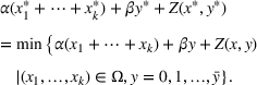
We propose an exact solution algorithm for problem P2S with a polynomial running time when the number of distinct arrival times of the prescheduled trucks at the store, k, is fixed. The idea of the algorithm is that we enumerate every possible number x_h of prescheduled trucks in B_h, for h = 1, …, k, and every possible number y of additional trucks that are used in a solution, and formulate the problem with every possible combination of the numbers of trucks used (x₁, …, x_k, y) as a linear program. We introduce some new notations and describe the algorithm in detail below.

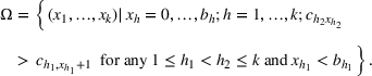
For h = 1, …, k and x_h = 0, …, b_h, we denote the subset of the x_h trucks in B_h with the largest spare capacities as B_h(x_h) = {(h, i) | i = 1, …, x_h}, where B_h(0) = ∅. By property (1) of Lemma 1, we know that if x_h prescheduled trucks in B_h are used in a solution for problem P2S, then they must be the trucks in B_h(x_h). In addition, by property (2) of Lemma 1, we know that the spare capacity of any used prescheduled truck is larger than that of any other unused prescheduled truck with an earlier arrival time at the store. Let Ω denote the set of all possible combinations of the numbers of prescheduled trucks used, denoted as (x₁,…, x_k). By Lemma 1, Ω can be calculated as follows:

Let

$\overline{y}=\lceil {\sum }_{j\in N}{w}_j/c_0\rceil$

denote the maximum number of additional trucks used in any feasible solution to problem P2S.

For every possible combination of (x₁, …, x_k, y), where (x₁, …, x_k) ∈ Ω and y ∈ {0, 1, …,

$\overline{y}$

}, we define a subproblem of P2S, denoted as P2S(x, y), where y additional trucks and the prescheduled trucks in B₁(x₁)

$\cup$

⋅⋅⋅

$\cup$

B_k(x_k) are used to transport the orders fulfilled at the FC. It is clear that the transportation cost of the orders fulfilled at the FC under (x₁, …, x_k, y) is fixed, which is α(x₁ + ⋅⋅⋅ + x_k) + βy. Hence, the objective of subproblem P2S(x, y) is to minimize the total processing cost of the orders fulfilled at the store. In the following, we show that each subproblem P2S(x, y) can be solved as a linear program. As described later, the overall problem P2S can be solved by first solving the subproblems P2S(x, y) under all possible combinations of (x₁, …, x_k, y), and then selecting the solution with the least total fulfillment cost.

We now show that each subproblem P2S(x, y) with given (x₁, …, x_k, y) can be formulated as a linear program. To start, for each j ∈ N, let θ_j = max{h | d_j ≥ τ_h, h = 1, …, k} such that order j can only be delivered by the trucks in set

$B_0\cup \cdots \cup B_{{\theta }_j}$

. For each h = 1, …, k, let A_h denote the set of orders that can be delivered by the prescheduled trucks in B_h, that is, A_h = {j ∈ N | d_j ≥ τ_h}. Let D_t denote the set of orders whose pickup ready times are no later than

${\overline{d}}_t$

, that is, D_t = {j ∈ N | d_j ≤

${\overline{d}}_t$

}, for t = 1, …, u. To formulate subproblem P2S(x, y), we introduce the following three sets of decision variables:

• q_jhi: The proportion of order j delivered by prescheduled truck (h, i) for j ∈ N, h = 1, …, θ_j, i = 1, …, x_h.

• r_jl: The proportion of order j delivered by additional truck l, for j ∈ N, l = 1, …, y.

• s_j: The proportion of order j fulfilled at the store, for j ∈ N.

Subproblem P2S(x, y) can be formulated as the following linear program:

$$\left[\mathrm{LP}-\mathrm{P}2\mathrm{S}\right]\min \sum _{j\in N}{\gamma }_j{s}_j,$$

1

$$\mathrm{s}.\mathrm{t}.\sum _{j\in A_h}{w}_j{q}_{\mathrm{jhi}}\le c_{\mathrm{hi}},h=1,\text{…},k;i=1,\text{…},x_h,$$

2

$$\sum _{j\in N}{w}_j{r}_{jl}\le c_0,l=1,\text{…},y,$$

3

$$\sum _{j\in D_t}{p}_j{s}_j\le {\overline{d}}_t,t=1,\text{…},u,$$

4

$$\sum _{h=1}^{{\theta }_j}\sum _{i=1}^{x_h}{q}_{\mathrm{jhi}}+\sum _{l=1}^y{r}_{\mathrm{jl}}+s_j=1,j\in N,$$

5

6

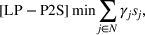
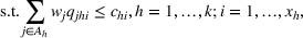
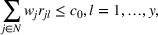
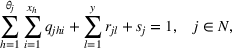
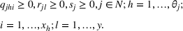
The objective of the above formulation (1) is to minimize the total processing cost of the orders fulfilled at the store. Constraints (2) and (3) restrict that the total size of orders assigned to each prescheduled truck and each additional truck does not exceed its capacity, respectively. Constraints (4) ensure that processing the orders assigned to the store in their NDPRT sequence will not violate their pickup ready times. Constraints (5) guarantee that each order in N is fulfilled. It is clear that the above formulation contains O(n²) variables and O(n) constraints.

Now, we describe the algorithm for solving problem P2S.

Algorithm A2 for Problem P2S :

• Step 1:

For every possible combination of (x₁, …, x_k, y), where (x₁, …, x_k) ∈ Ω and y ∈ {0, 1, …,

$\overline{y}$

}, solve subproblem P2S(x, y) by solving the LP problem [LP‐P2S]. Denote the optimal objective value of subproblem P2S(x, y) as Z(x, y).

Step 2:

Find optimal solution

$(x_1^{\ast },\text{…},x_k^{\ast },y^{\ast })$

such that

Adopt the following solution for P2S: use all the prescheduled trucks in

$B_h(x_h^{\ast })$

, for h = 1, …, k, and y^* additional trucks, and assign the orders to the trucks and the store following the optimal solution of the subproblem P2S(x^*, y^*).

Theorem 5

Algorithm A2 finds an optimal solution for problem P2S in

$O(n{(m/k)}^k{T}_{LP})$

time, where T_LP is the running time of the LP problem [LP‐P2S].

Theorem 5 indicates that when the number of distinct arrival times of the prescheduled trucks at the store, k, is fixed, problem P2S can be solved to optimality in polynomial time by Algorithm A2.

Before we end this section, we show a property about the LP formulation [LP‐P2S], which is used in Section 5.3 when we design a heuristic for problem P2N. Lemma 5

In any optimal basic solution of [LP‐P2S] for subproblem P2S(x, y), there are at least

$\left(n-{\sum }_{h=1}^k{x}_h-y-u\right)$

q_jhi, r_jl, and s_j variables taking the value 1.

Solving problem P2S with arbitrary k

We propose a pseudo‐polynomial time dynamic programming algorithm for solving problem P2S with an arbitrary k. The algorithm is comprised of three stages, each of which solves a different special case of problem P2S, respectively. In Stage 1, we solve the special case of P2S where all the orders are fulfilled at the store. In Stage 2, we solve the special case of P2S where at least one unit of an order is fulfilled at the FC, and the orders and suborders fulfilled at the FC are all delivered by additional trucks only. In Stage 3, we solve the special case of P2S, where at least one unit of an order is fulfilled at the FC and delivered by a prescheduled truck, and the orders and suborders fulfilled at the FC can be delivered by both the prescheduled trucks and additional trucks. Clearly, the lowest cost one of the three schedules generated in the three stages is optimal for P2S.

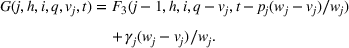
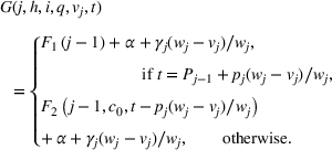
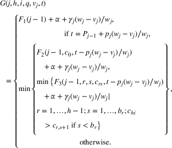
The Stage 1 problem is trivial, since, from Lemma 2 we know that processing all the orders in N at the store in the NDPRT sequence is optimal for this problem, provided that this schedule is feasible. For the problems in Stages 2 and 3, the idea of the algorithm is the following. Based on Lemmas 1–3, we can consider orders in the NDPRT sequence one by one. When an order is considered, all three possible fulfillment options are compared: (i) it is fully fulfilled at the FC, (ii) it is fully fulfilled at the store, and (iii) it is partially fulfilled at the FC and partially fulfilled at the store. For Stage 2, we use additional trucks to deliver all the orders and suborders that are fulfilled at the FC, and an order fulfilled at the FC must be delivered by the last additional truck used if it has enough remaining capacity, and by the last additional truck used and a new additional truck if the last additional truck used does not have enough capacity. For Stage 3, we use both the prescheduled trucks and additional trucks, which are considered one by one in the following sequence: additional trucks first, followed by prescheduled trucks in B₁, B₂, …, B_k in this order. Delivery of an order fulfilled at the FC has three options: (a) if no prescheduled truck is used yet, then the order can be delivered entirely by one or two additional trucks, or partly by an additional truck and partly by a prescheduled truck; (b) if some prescheduled trucks have already been used, then the order must be delivered by one or two prescheduled trucks.

Algorithm DP1 for Problem P2S :

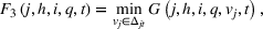
Reindex the orders in N in the NDPRT sequence. Let

$P_j={\sum }_{l=1}^j{p}_j$

, and θ_j = max{h | d_j ≥ τ_h, h = 0, …, k}, for j = 1, …, n. Thus, order j can only be delivered by the trucks in set

$B_0\cup \cdots \cup B_{{\theta }_j}$

.

Stage 1 :

Define F₁(j) as the minimum fulfillment cost of a partial schedule comprised of orders 1, …, j, where all these orders are fulfilled at the store, for j ∈ N. To calculate F₁(j) for each j, we generate a schedule where orders 1, …, j, are processed at the store in the NDPRT sequence. If under this schedule, the pickup ready times of all the orders are satisfied, then let F₁(j)

$={\sum }_{l=1}^j{\gamma }_l$

; otherwise, let F₁(j) = ∞. The optimal schedule of Stage 1 is that corresponds to F₁(n).

Stage 2 :

Value functions: Define F₂(j, q, t) as the minimum total cost of a partial schedule where (i) the first j orders, 1, …, j, have been fulfilled at the FC and loaded to some additional trucks, or fulfilled at the store, (ii) the last additional truck used is loaded with q units of orders, where 1 ≤ q ≤ c₀, and (iii) the completion time of the last order processed at the store is t.

Boundary conditions:

Recursive relations: For j = 2, …, n; q = 1, …, c₀; t = 0, 1, …, min{d_j, P_j}:

where Δ _jt = {e | p_j(w_j − e) / w_j ≤ t, e = 0, 1, …, w_j} is the set of all values of e such that processing (w_j − e) units of order j at the store takes no longer than t time units.

Optimal objective value:

$\min \{F_2(n,q,t)|q=1,\text{…},c_0;t=0,\text{…},\min \{d_n,P_n\}\}$

.

Stage 3 :

Value function: Define F₃(j, h, i, q, t) as the minimum total cost of a partial schedule where (i) the first j orders, 1, …, j, have been fulfilled at the FC and loaded to some additional trucks and some prescheduled trucks, or fulfilled at the store; (ii) the last truck used is prescheduled truck (h, i), and it is loaded with q units of orders, where 1 ≤ q ≤ c_hi, and (iii) the completion time of the last order processed at the store is t.

Boundary conditions:

Recursive relations: For j = 1, …, n; h = 1, …, θ_j; i = 1, …, b_h; q = 1, …, c_hi; t = 0, 1, …, min{d_j, P_j}:

$$F_3\left(j,h,i,q,t\right)=\underset{v_j\in {\mathrm{\Delta }}_{jt}}{\min }G\left(j,h,i,q,v_j,t\right),$$

where Δ _jt is defined the same way as in Stage 2, and there are three cases for calculating

$G(h,i,j,q,v_j,t)$

:

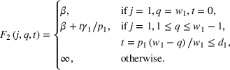
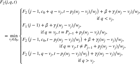
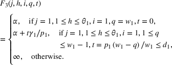
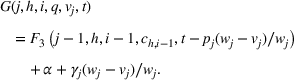
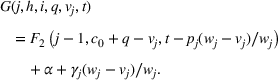
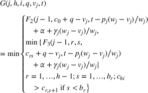
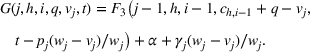
• If q > v_j, then

  

• If q = v_j, then we further distinguish three subcases:

• b.2

  If h ≥ 2 and i = 1, then

  

• b.3

  If i ≥ 2, then

  

If q < v_j, we also distinguish three subcases:

• c.1

If h = 1 and i = 1, then

c.2

If h ≥ 2 and i = 1, then

c.3

If i ≥ 2, then

Optimal objective value:

$\min \{F_2(n,h,i,q,t)|h=1,\text{…},k;i=1,\text{…},b_h;q=1,\text{…},c_{hi};t=0,\text{…},\min \{d_n,P_n\}\}$

. Theorem 6

Algorithm DP1 solves problem P2S in O(m²nc₀Pw_max) time, where

$P={\sum }_{j\in N}{p}_j$

and w_max = max_j∈N w_j.

From this theorem, we observe that problem P2S with an arbitrary k is at most ordinarily NP‐hard. It is open whether this problem is exactly ordinarily NP‐hard or polynomially solvable.

Solving problem P2N with fixed k

We propose a polynomial‐time heuristic for solving problem P2N with a fixed k. The heuristic constructs a feasible solution for P2N based on the optimal solution of problem P2S obtained by Algorithm A2.

Heuristic H2 for Problem P2N :

Step 1: Solve problem P2S by Algorithm A2 to obtain an optimal solution

$(x_1^{\ast },\text{…},x_k^{\ast },y^{\ast })$

for the trucks used from B₁, …, B_k and B₀, respectively, and a corresponding optimal basic solution (q^*, r^*, s^*) obtained for the subproblem P2S (x^*, y^*). Under this optimal basic solution, let N₁ denote the set of orders entirely assigned to a prescheduled truck, N₂ the set of orders entirely assigned to an additional truck, and N₃ the set of orders entirely assigned to the store, that is,

$$N_2=\{j\in N|r_{\mathrm{jl}}^{*}=1,\mathrm{for}\mathrm{some}l=1,\text{…},y^{*},$$

$$N_3=\{j\in N|s_j^{\ast }=1\}.$$

Let N₄ = N ∖ (N₁

$\cup$

N₂

$\cup$

N₃) denote the set of orders that are split (i.e., assigned among multiple trucks or among some trucks and the store).

Step 2: Construct a feasible solution π₁ for the jobs in N₁

$\cup$

N₂

$\cup$

N₃ based on (q^*, r^*, s^*) as follows. Pack each order j ∈ N₁ into prescheduled truck (h, i) with

$q_{jhi}^{\ast }=1$

, and pack each order j ∈ N₂ into additional truck l with

$r_{jl}^{\ast }=1$

. Fulfill the orders in N₃ at the store by processing them in the NDPRT sequence. Let Ψ denote the set of the prescheduled trucks and additional trucks currently used.

Step 3: Construct a feasible solution π for problem P2N by assigning the jobs in N₄ to the trucks in Ψ and possibly new trucks as follows. We consider the orders in N₄ in the nonincreasing sequence of their sizes w_j. For each order j ∈ N₄ in this sequence, we first try to pack it into any truck in Ψ whose arrival time at the store is no later than d_j. If no such truck in Ψ can carry order j, we then first select a prescheduled truck (h, i) with h ≤ θ_j that has not been used so far, pack this order to it and add this new prescheduled truck to Ψ. If no such prescheduled truck exists, then use a new additional truck, pack this order into it, and add this new additional truck to Ψ.

Clearly, Step 1 of Heuristic H2 is the most time‐consuming step. Hence, the overall time complexity of Heuristic H2 is the same as that of Algorithm A2, which is

$O(n{(m/k)}^k{T}_{LP})$

. Thus, when k is fixed, this heuristic has a polynomial running time. Theorem 7

The worst‐case performance ratio of Heuristic H2 for problem P2N is bounded by 1 + β (u + 1)/α.

Remark 1

For a special case of P2N where all the orders have a common pickup ready time, that is, u = 1, the worst‐case performance ratio of Heuristic H2 is bounded by 1 + 2β/α.

Theorem 8

The asymptotic worst‐case performance ratio of H2 for problem P2N is bounded by 2 when the number of prescheduled trucks

$m$

and the number of distinct order pickup ready times

$u$

are both fixed.

To enhance Heuristic H2, we propose in Appendix A2 (Supporting Information) an efficient local search procedure, denoted as H2‐LS, which takes the solution from H2 for problem P2N and improves it by simple local search schemes.

Solving problem P2N with arbitrary k

In this section, we propose a pseudo‐polynomial time heuristic for problem P2N where k is arbitrary. The idea of the heuristic is that we first solve a relaxed version of problem P2N by a pseudo‐polynomial time algorithm, and then construct a feasible solution for problem P2N based on the optimal solution for this relaxed problem.

Consider a relaxed version of problem P2N, where order delivery is splittable, that is, it can be delivered by multiple prescheduled trucks or multiple additional trucks, but not by a mixture of prescheduled and additional trucks. All the other characteristics of the relaxed problem are exactly the same as in problem P2N. Denote this problem as P2N′. We note that problem P2N′ is more restrictive than problem P2S and differs from the latter in two major ways. Unlike in problem P2S, in problem P2N′, (i) order processing is not splittable, that is, an order must be processed either at the store or at the FC, (ii) an order cannot be delivered by a mixture of prescheduled and additional trucks.

Let

$F_{P2N^{\prime }}^{\ast }$

denote the optimal objective value of P2N′. We have the following result. Lemma 6

$F_{P2N}^{\ast }\ge F_{P2N^{\prime }}^{\ast }$

.

Lemma 6 can be proved in a similar way as Lemma 4. To solve problem P2N′, we propose a pseudo‐polynomial time DP algorithm, denoted as DP2, which is comprised of four stages. Each stage considers a different special case of problem P2N′. The optimal solution for problem P2N′ is the one among the four schedules generated from these four stages, whose total cost is the lowest. The details of DP2 are provided in Appendix A2 (Supporting Information). In the following, we first show a result about DP2. Lemma 7

Algorithm DP2 finds an optimal solution for Problem P2N′ in

$O(n{m}^2{c}_0^2{P}_n)$

time, where if K ≥ 1 prescheduled trucks are used, then at most K − 1 orders are delivered by multiple prescheduled trucks.

Next, we propose a heuristic for problem P2N, which constructs a feasible solution for problem P2N based on the optimal solution obtained by algorithm DP2 for problem P2N′.

Heuristic H3 for Problem P2N :

Step 1: Solve problem P2N′ by Algorithm DP2 and obtain solution σ. In solution σ, let N₁ denote the set of orders, each of which is assigned to a single prescheduled truck, N₂ the set of orders assigned to additional trucks, N₃ the set of orders fulfilled at the store, and N₄ the set of orders, each of which is assigned to multiple prescheduled trucks. Let L denote the number of additional trucks and K the number of prescheduled trucks used in σ.

Step 2: Create a solution π for problem P2N based on σ as follows. For the orders in N₁

$\cup$

N₃, use the same solution for them as in σ. For the orders in N₂, the use of the first fit decreasing or best fit decreasing heuristic for the bin packing problem (e.g., Coffman et al., 1997) to assign these orders to additional trucks. Let Ψ denote the set of trucks packed with orders in N₁

$\cup$

N₂ so far. Finally, for the orders in N₄, we first sort them in the nonincreasing sequence of their sizes w_j. For each order j ∈ N₄ in this sequence, we first try to pack it into any truck (h, i) ∈ Ψ whose arrival time at the store is no later than d_j. If no such truck in Ψ can carry order j, then we first select a prescheduled truck (h, i) with h_j ≤ θ_j that has not been used so far, pack this order into this truck and add this truck to Ψ. If no such prescheduled truck exists, we pack order j into a new additional truck and add this truck to Ψ. Theorem 9

The worst‐case performance ratio of heuristic H3 for problem P2N is bounded by 1 + β /α.

Theorem 10

The asymptotic worst‐case performance ratio of heuristic H3 for problem P2N is bounded by 2 when the number of prescheduled trucks m is fixed.

We note that the local search procedure H2‐LS developed for improving the solution from H2 (given in Appendix A2, Supporting Information) can also be used to improve the solution from H3 for problem P2N. The resulting local search is denoted as H3‐LS.

COMPUTATIONAL EXPERIMENTS

In this section, we conduct computational experiments to evaluate the performance of the proposed heuristics and derive managerial insights. We first describe in Section 6.1 how the test instances are generated based on real‐world practices. In Section 6.2, we evaluate the performance of the heuristics for problems P1N and P2N by comparing their solutions with the lower bounds obtained by solving the corresponding splittable version of the problems, P1S and P2S. The effectiveness of the local search procedures described in Appendix A2 (Supporting Information) is also evaluated. In Sections 6.3 and 6.4, we derive several managerial insights regarding the impact of the prescheduled trucks and the impact of the order processing costs at the store, respectively. In Section 6.5, we consider a dynamic version of the studied problems where orders arrive randomly over time and demonstrate how our proposed algorithms can be implemented to solve such dynamic problems using a rolling horizon strategy. All the algorithms are implemented in C++, where the linear programs involved in H2 are solved by Gurobi 9.0.2 under the default setting. The experiments are conducted on a PC with 16 GB RAM and an Intel(R) Core(TM) i7‐8565U CPU operating at 1.8 GHz.

Test instances

We generate test instances following widely adopted practices for fulfilling BOPS orders in OCR. The decisions in such a setting are usually made on a rolling horizon basis (e.g., MacCarthy et al., 2019). As discussed in Section 1, many retailers promise a short pickup ready time, varying from 2 hours to 1 day, from the time when an order is placed. Thus, it is reasonable to assume that in an average setting, the promised pickup ready time of each order is 4 hours from the time it is placed. Accordingly, we assume that the decisions are made every 3 hours in order to have enough time to generate a solution that meets the pickup ready time of every order received in the last 3 hours. Thus, we consider the problems defined in a 3‐hour time horizon. Let the current time be 0. Considering the orders received in the last 3 hours, given the above‐discussed 4‐hour window within which an order must be ready for pickup, we can see that orders received 3 − x hours earlier have a pickup ready time of 4 − (3 − x) = 1 + x hours from now, where 0 ≤ x ≤ 3 and the number of different x values correspond to the number of distinct order pickup ready times u. Following this basic setting, we generate the test instances as follows.

The number of orders n ∈ {50, 100, 200}. The size w_j of each order j is randomly drawn from U[1, 10], where

$U[\underline{a},\overline{a}]$

denotes the uniform distribution over interval

$[\underline{a},\overline{a}]$

. The processing time p_j of order j at the store is randomly generated from U[1, 10] minutes, while its fulfillment cost at the store γ_j is set as δw_j, where δ is a parameter randomly generated from U[0.5, 1.5] unless otherwise specified.

The number of distinct order pickup ready times u ∈ {1, 3, 5}. For each u, we set the pickup ready time d_j of each order j as 1 + x hours from the current time 0, where x is randomly selected from {3} when u = 1, from {0, 1, 2} when u = 3, and from {0.5, 1, 1.5, 2, 2.5} when u = 5.

The number of prescheduled truck sets k depends on the value of u. Recall from Section 3 that without loss of generality, it can be assumed that k ≤ u. Thus, we test k ∈ {1} when u = 1, test k ∈ {1, 3} when u = 3, and test k ∈ {1, 3, 5} when u = 5. For each pair of (u, k) considered, we first determine the latest order pickup ready time, denoted as d_max. We then randomly sample k distinct time points τ₁, …, τ_k from interval [0, d_max] as the arrival times of prescheduled trucks in B₁, …, B_k, respectively, where τ₁ < ⋅⋅⋅ < τ_k. For each h (1 ≤ h ≤ k), we randomly generate the number of prescheduled trucks in B_h from U[1, 2].

The capacity of each additional truck c₀ is set as 100, and the cost for using each additional truck β as 100. We observe that given the values of c₀ and β, as specified here, if δ < 1, then it is generally less costly to fulfill an order at the store, and if δ > 1, then it is generally less costly to fulfill an order at the FC.

The spare capacity of a prescheduled truck c_hi is randomly generated from U[10, 30]. This represents the reality that a prescheduled truck usually has a spare capacity of 10–30%. Paul et al. (2019b) make a similar assumption. We consider two cases of the fixed cost of using a prescheduled truck α, that is, α ∈ {5, 10}. We observe that given the ranges of α and c_hi and the values of β and c₀, it is much less costly to use a prescheduled truck than an additional truck, which is often the case in practice, as discussed in Section 1.

Performance of the heuristics

In this section, we report the computational results of heuristics H1 and H1‐LS for solving problem P1N, and heuristics H2, H2‐LS, H3, and H3‐LS for solving problem P2N, in Tables 1, 2, and 3, respectively. For each problem, we randomly generate 10 test instances for each combination of (n, u, k) and α and report under column “G_avg” (respectively “G_max”) the average (respectively maximum) optimality gap (%) of each tested heuristic H, that is, (F^H − F^LB)/ F^LB × 100%, where F^H is the total cost of the solution generated by heuristic H and F^LB is the lower bound of the optimal objective value of the instance obtained by solving the corresponding splittable problem. We note that the computational time of H1 for solving every instance is less than 0.01 s, thus is not reported. We also note that the local search procedures take less than 0.01 s for all the test instances. Hence, we only report under column “Time” the average computational times (in seconds) of H2 and H3 in Tables 2 and 3, respectively.

TABLE 1

Computational results of H1 for problem P1N

	α = 5				α = 10
	H1		H1‐LS		H1		H1‐LS
(n, u, k)	G avg	G max	G avg	G max	G avg	G max	G avg	G max
(50, 1, 1)	3.61	32.79	0.33	1.67	3.89	32.26	0.67	3.33
(50, 3, 1)	3.45	32.79	0.17	1.67	3.56	32.26	0.33	3.33
(50, 3, 3)	5.17	45.45	0.62	2.33	5.33	41.67	1.17	4.35
(50, 5, 1)	3.61	32.79	0.33	1.67	3.89	32.26	0.67	3.33
(50, 5, 3)	4.82	46.51	0.17	1.67	4.68	43.48	0.33	3.33
(50, 5, 5)	24.62	68.97	5.97	48.28	22.09	52.63	4.22	21.05
(100, 1, 1)	1.74	17.36	0.00	0.00	1.80	18.03	0.00	0.00
(100, 3, 1)	0.08	0.83	0.08	0.83	0.16	1.64	0.16	1.64
(100, 3, 3)	4.74	23.26	0.39	0.98	4.98	21.74	0.76	1.92
(100, 5, 1)	0.08	0.83	0.08	0.83	0.16	1.64	0.16	1.64
(100, 5, 3)	6.39	23.26	0.20	0.98	6.30	21.74	0.38	1.92
(100, 5, 5)	5.07	24.14	2.20	18.18	5.16	23.40	1.98	12.50
(200, 1, 1)	1.95	9.05	0.14	0.45	2.07	9.01	0.27	0.91
(200, 3, 1)	3.67	9.09	0.09	0.45	3.71	9.09	0.18	0.91
(200, 3, 3)	2.33	9.80	0.32	0.91	2.65	9.62	0.64	1.80
(200, 5, 1)	2.95	9.55	0.18	0.91	3.17	10.00	0.36	1.82
(200, 5, 3)	5.16	10.78	0.42	0.91	5.49	11.54	0.82	1.82
(200, 5, 5)	3.78	10.64	1.54	8.51	4.42	11.22	1.95	6.12
Average	4.62	22.66	0.73	5.07	4.64	21.29	0.84	3.99

TABLE 2

Computational results of H2 for problem P2N

	α = 5					α = 10
	H2			H2‐LS		H2			H2‐LS
(n, u, k)	G avg	G max	Time	G avg	G max	G avg	G max	Time	G avg	G max
(50, 1, 1)	45.22	49.73	0.01	0.96	3.98	39.61	47.18	0.01	0.98	3.88
(50, 3, 1)	44.20	49.73	0.01	5.20	24.26	39.56	48.31	0.01	4.52	21.26
(50, 3, 3)	54.68	62.50	0.03	10.07	46.01	44.67	55.15	0.04	6.64	29.26
(50, 5, 1)	44.84	50.00	0.01	5.80	21.21	39.06	47.55	0.01	4.85	18.64
(50, 5, 3)	58.62	85.47	0.03	18.15	47.22	46.91	68.03	0.03	7.84	28.40
(50, 5, 5)	77.99	98.02	0.14	19.81	54.01	48.62	72.18	0.12	11.33	28.82
(100, 1, 1)	21.67	23.92	0.03	2.91	11.80	19.29	23.42	0.02	2.34	9.37
(100, 3, 1)	20.96	24.13	0.02	2.96	11.22	20.63	23.54	0.02	2.46	8.68
(100, 3, 3)	23.10	26.18	0.12	8.42	19.22	19.98	24.83	0.11	4.79	11.31
(100, 5, 1)	21.17	23.50	0.02	0.97	2.14	21.00	23.31	0.02	0.75	1.95
(100, 5, 3)	23.92	27.92	0.12	2.74	14.29	22.38	24.81	0.12	2.29	9.40
(100, 5, 5)	27.34	30.95	0.46	12.23	23.62	25.73	30.08	0.44	4.01	16.77
(200, 1, 1)	9.85	10.20	0.14	0.59	1.06	9.95	11.37	0.14	0.53	0.98
(200, 3, 1)	9.61	10.47	0.12	1.56	6.02	9.61	10.50	0.12	1.30	4.97
(200, 3, 3)	9.95	10.83	0.56	3.00	7.02	9.95	11.00	0.53	1.77	5.33
(200, 5, 1)	9.79	10.76	0.12	0.88	5.78	9.75	10.64	0.13	0.40	1.04
(200, 5, 3)	10.14	10.65	0.59	3.89	8.52	10.05	11.13	0.58	2.31	6.26
(200, 5, 5)	10.68	12.00	4.59	5.75	9.24	10.39	12.27	4.39	2.67	5.24
Average	29.10	34.28	0.40	5.88	17.59	24.84	30.85	0.38	3.43	11.75

TABLE 3

Computational results of H3 for problem P2N

	α = 5					α = 10
	H3			H3‐LS		H3			H3‐LS
(n, u, k)	G avg	G max	Time	G avg	G max	G avg	G max	Time	G avg	G max
(50, 1, 1)	4.31	43.10	1.35	0.17	1.72	4.60	41.32	0.94	0.17	1.65
(50, 3, 1)	5.08	50.76	1.02	2.34	23.35	5.23	48.31	0.74	1.74	17.39
(50, 3, 3)	40.73	65.79	3.18	12.86	44.79	26.88	56.50	3.60	7.78	28.19
(50, 5, 1)	4.31	43.10	1.00	0.09	0.86	4.60	41.32	1.00	0.08	0.83
(50, 5, 3)	45.32	85.47	3.87	11.56	44.71	34.90	68.03	3.80	8.28	28.72
(50, 5, 5)	81.60	102.04	5.77	20.45	56.93	58.44	75.19	5.60	12.08	32.18
(100, 1, 1)	0.00	0.00	3.50	0.00	0.00	0.24	2.35	3.11	0.00	0.00
(100, 3, 1)	0.00	0.00	2.09	0.00	0.00	0.00	0.00	2.01	0.00	0.00
(100, 3, 3)	0.00	0.00	5.47	0.00	0.00	0.48	2.52	5.22	0.00	0.00
(100, 5, 1)	0.00	0.00	2.13	0.00	0.00	0.23	2.33	2.03	0.00	0.00
(100, 5, 3)	2.45	24.51	6.54	0.07	0.74	2.80	23.09	6.08	0.07	0.69
(100, 5, 5)	8.34	30.30	17.92	2.18	20.93	4.41	26.67	18.57	0.16	1.11
(200, 1, 1)	0.00	0.00	10.05	0.00	0.00	0.21	1.05	10.01	0.00	0.00
(200, 3, 1)	0.00	0.00	6.73	0.00	0.00	0.10	1.00	6.54	0.00	0.00
(200, 3, 3)	0.00	0.00	66.79	0.00	0.00	0.11	1.08	66.35	0.00	0.00
(200, 5, 1)	0.00	0.00	6.81	0.00	0.00	0.20	1.04	7.22	0.00	0.00
(200, 5, 3)	0.00	0.00	77.45	0.00	0.00	0.31	1.05	73.62	0.08	0.83
(200, 5, 5)	0.00	0.00	220.73	0.00	0.00	0.23	1.15	217.82	0.05	0.45
Average	10.67	24.73	24.58	2.76	10.78	8.00	21.89	24.12	1.69	6.22

From Tables 1–3, we can observe the following findings. First, heuristics H1, H2 and H3 without the added local search procedures already perform reasonably well, especially for large test instances. H1 and H3 are capable of generating solutions with a small optimality gap for most test instances of any size in short computational time, and H2 performs well for most test instances with 200 orders. Second, by comparing the results of H1, H2, and H3 with those of H1‐LS, H2‐LS, and H3‐LS, respectively, we can see that the local search procedures significantly improve the quality of the solutions generated by the heuristics H1, H2 and H3. In fact, the average optimality gaps of the solutions generated by H1‐LS, H2‐LS, and H3‐LS across all combinations of (n, u, k) and α are no more than 5.88%. Third, for problem P2N, heuristics H3 and H3‐LS generate much higher quality solutions than H2 and H2‐LS, respectively, with slightly more computational time. For almost all the instances with 200 orders, the solutions generated by H3 and H3‐LS are optimal. Fourth, as the number of orders n gets larger, all the heuristics perform generally better. However, as the number of order pickup ready times u and the number of prescheduled truck sets k to become larger, all the heuristics perform generally worse, although their overall performances are still very good. This implies that the more diverse the order pickup ready times or the prescheduled trucks are, the more challenging the problems are. Finally, the optimality gaps of H2 and H3 decrease generally with the fixed cost of using a prescheduled truck α, which is consistent with the fact that their worst‐case performance ratios (see Theorems 7 and 9) decrease with α. However, in the case of H1, we do not observe a similar result. This is not surprising because the worst‐case behavior of an algorithm does not necessarily represent the overall performance of the algorithm over a large number of test instances.

Impact of the prescheduled trucks

In this section, we study the impact of the presence of prescheduled trucks on the total fulfillment cost by comparing the total cost of a problem with the prescheduled trucks and the total cost of the same problem but without the prescheduled trucks. In our experiments, we fix u = 5 and test k ∈ {1, 3, 5} to reflect the situations with different numbers of available prescheduled trucks. We generate 10 random instances for each combination of (n, k) and α. For each generated instance, we calculate the relative cost reduction R due to the use of prescheduled trucks (or, the benefit brought by the prescheduled trucks), defined as R = (F − F′)/F′ × 100%, where F is the total cost of the solution generated by heuristic H1‐LS (respectively H3‐LS) for problem P1N (respectively P2N) with the prescheduled trucks, and F′ is that of the solution generated by H1‐LS (respectively H3‐LS) when no prescheduled trucks are available. In the latter case, the solution and F′ are generated by first setting b_h = 0, for h = 1, …, k, and then rerunning the corresponding heuristic. The results are reported in Table 4, where for each combination of (n, k) and α, we report under columns “#pre” and “#add” the average numbers of prescheduled trucks and additional trucks used, respectively, for the problem with the prescheduled trucks, under column “#add′” the average number of additional trucks used for the problem without the prescheduled trucks, under column “R_avg” the average relative cost reduction (%) brought by using prescheduled trucks over the 10 tested instances.

TABLE 4

Impact of the prescheduled trucks on the solutions for problems P1N and P2N

		α = 5				α = 10
	(n, k)	#pre	#add	#add′	R avg	#pre	#add	#add′	R avg
P1N	(50, 1)	0.3	3.0	3.1	2.38	0.3	3.0	3.1	2.25
	(50, 3)	2.4	2.4	3.1	18.71	2.4	2.4	3.1	14.92
	(50, 5)	4.9	1.9	3.1	30.37	4.9	1.9	3.1	22.42
	(100, 1)	0.3	5.9	6.1	2.87	0.3	5.9	6.1	2.64
	(100, 3)	2.7	5.1	6.1	14.19	2.7	5.1	6.1	11.95
	(100, 5)	4.7	4.7	6.1	19.02	4.7	4.7	6.1	15.19
	(200, 1)	0.6	11.2	11.5	2.33	0.6	11.2	11.5	2.17
	(200, 3)	3.1	10.6	11.5	6.52	3.1	10.6	11.5	5.30
	(200, 5)	6.1	10.0	11.5	10.24	6.1	10.0	11.5	7.60
	Average	2.8	6.1	6.9	11.85	2.8	6.1	6.9	9.38
P2N	(50, 1)	1.4	1.0	1.2	10.39	1.3	1.0	1.2	7.42
	(50, 3)	3.8	0.6	1.2	22.59	3.5	0.6	1.2	14.20
	(50, 5)	6.1	0.3	1.2	34.76	5.5	0.3	1.2	22.01
	(100, 1)	1.4	3.2	3.7	5.40	1.3	3.2	3.7	3.93
	(100, 3)	4.5	2.6	3.7	14.95	4.3	2.6	3.7	10.19
	(100, 5)	7.2	2.2	3.7	23.97	7.1	2.1	3.7	17.50
	(200, 1)	1.5	8.3	8.5	2.23	1.3	8.4	8.5	1.47
	(200, 3)	4.1	7.9	8.5	5.82	3.8	7.9	8.5	3.71
	(200, 5)	7.7	7.1	8.5	11.35	7.5	7.1	8.5	7.48
	Average	4.2	3.7	4.5	14.61	4.0	3.7	4.5	9.77

We can make several observations from Table 4. First, there is a significant cost reduction (varying from 9.38% to 14.61% on average basis) due to the use of prescheduled trucks in both problems P1N and P2N. This means that if there are prescheduled trucks available, retailers should take advantage of them to reduce total fulfillment cost when dealing with BOPS orders. Second, as the fixed cost of using a prescheduled truck α decreases, the average relative cost reduction due to the prescheduled trucks increases in all cases of (n, k) of both problems. This is simply because the total cost for using the prescheduled trucks is lower when α decreases. Similarly, as the number of available prescheduled trucks (reflected by k) increases, the cost reduction generally increases. This is because the more the available prescheduled trucks, the more potential cost reduction they can bring. Finally, by comparing the cost reductions between problems P1N and P2N, we can see that the existence of the store fulfillment option (as in problem P2N) increases the number of prescheduled trucks used and hence amplifies the cost reduction that can be brought by the prescheduled trucks.

Impact of the order fulfillment costs at the store

In this section, we study the impact of the order fulfillment costs γ_j at the store in problem P2N. To this end, we fix α as 10 and consider three different values of δ, that is, δ ∈ {0.5, 1, 1.5}, where, as defined in Section 7.1, a larger value of δ represents higher order fulfillment costs γ_j at the store. For each combination of (n, u, k) and δ, we generate 10 random instances and solve each instance using H3‐LS. The results are reported in Table 5, where column “#store” is the average number of orders fulfilled at the store, and column “C_store” is the average total cost of the orders fulfilled at the store. We also report under column “R_avg” the average relative cost reduction R due to the presence of the store fulfillment option (or, the benefit of having the store fulfillment option), defined as R = (F^{P1 N} − F^{P2 N} )/F^{P1 N}  × 100%, where F^{P1 N} (respectively F^{P2 N} ) is the total cost of the solution generated by heuristic H1‐LS (respectively H3‐LS) for each instance where orders cannot (respectively can) be fulfilled at the store. The average optimality gaps of both H1‐LS and H3‐LS across all problem scales (n, u, k) are less than 2% for all three δ values. The average computational time of H1‐LS across all problem scales for each δ is no more than 0.01 second, while that of H3‐LS is no more than 32 seconds.

TABLE 5

Impact of the fulfillment costs at the store on the solutions of problem P2N

	δ = 0.5			δ = 1			δ = 1.5
(n, u, k)	#store	C store	R avg	#store	C store	R avg	#store	C store	R avg
(50, 1, 1)	26.4	74.8	45.6	17.5	126.6	16.43	11.9	48.1	12.63
(50, 3, 1)	22.9	62.3	42.43	8.4	65.9	16.67	9.2	39.1	12.62
(50, 3, 3)	21.7	61.8	37.46	14.7	107.1	10.01	5	30.2	5.52
(50, 5, 1)	23.4	61.2	42.8	5.9	46.1	16.6	11.7	51	12
(50, 5, 3)	26.9	81.2	43.1	20.9	147.7	10.41	6.5	36.7	6.39
(50, 5, 5)	26.4	75.9	47.68	18.6	141	13.05	3.8	23.1	12.07
(100, 1, 1)	39	123.5	32.45	6.3	56	6.11	14.7	57	3.33
(100, 3, 1)	30	91.1	25.68	6.3	56	5.93	12.2	44.9	3.46
(100, 3, 3)	29.9	90.2	24.97	7.8	67	4.62	8.3	30	2.75
(100, 5, 1)	34.9	105.1	28.47	6.3	56	5.93	14.5	55.5	3.2
(100, 5, 3)	35.5	112.2	29.65	7.5	65.8	4.3	8.6	30.5	2.28
(100, 5, 5)	35.4	115.2	31.98	8.5	67.7	6.76	8.7	32.4	4.68
(200, 1, 1)	47.4	152.1	20.06	6	53.8	3.33	10	21.7	2.91
(200, 3, 1)	35.6	111.2	15.83	6	53.8	3.42	10.6	21.4	3.02
(200, 3, 3)	35.8	119.9	17.55	4.7	43	4.42	13.6	31.5	3.89
(200, 5, 1)	42	140.7	18.49	6	53.8	3.33	10.2	21.6	2.92
(200, 5, 3)	41.9	143.8	19.12	4.7	43	4.07	12.6	32.1	3.48
(200, 5, 5)	41.8	140.1	18.86	8.4	77.9	3.31	13.8	52.5	2.09
Average	33.16	103.46	30.12	9.14	73.79	7.71	10.33	36.63	5.51

There are several observations that can be made from Table 5. First, we can see from column “R_avg” that the option of store fulfillment can significantly reduce the total fulfillment cost of BOPS orders, especially when the order fulfillment costs at the store γ_j are relatively low. For example, when δ = 0.5, the store fulfillment option can reduce the total cost by 30.12% on average. Even when δ = 1.5 (which represents the case where the average fulfillment cost at the store for an order is higher than that at the FC), the presence of the store fulfillment option can still reduce the total cost by 5.51% on average. Second, the cost reduction brought by the store fulfillment option is more significant for problems with fewer orders. This can be explained as follows. If δ < 1, it is generally cheaper to fulfill an order at the store. In this case, due to the limited store fulfillment capacity, when there are fewer orders, the relative cost reduction brought by the store fulfillment option becomes more significant. If δ ≥ 1, it is generally cheaper to fulfill an order at the FC. In this case, it is desirable to fully load a truck whenever possible, and fulfill the remaining few orders at the store. For example, we can see from columns “#store” and “C_store” under δ = 1.5 that the number of orders fulfilled at the store as well as their fulfillment costs is generally stable for all problem scales, thus making the cost reduction more significant for problems with fewer orders.

Applying our algorithms in a dynamic setting

In this section, we first describe a dynamic version of the static problems P1N and P2N studied above and then discuss how our algorithms developed for P1N and P2N can be applied in such a dynamic setting. Let P1N‐D and P2N‐D denote the dynamic version of problems P1N and P2N, respectively. In these dynamic problems, each order j ∈ N arrives over time during a given planning horizon with a known arrival time a_j. Let T denote the length of the planning horizon, which is set as 12 hours in our experiments. Following the setup given in Section 6.1, we assume that each order is promised an identical lead time L (i.e., 4 hours) for pickup at the store upon its arrival, which means that the pickup ready time of order j is d_j = a_j + L. In the dynamic setting, we need to explicitly consider the transportation time for a truck to travel from the FC to the store, which is denoted as Δ and set as 1 hour in our experiments. The additional trucks can depart from the FC at any desired time, whereas the prescheduled trucks can only depart at their specific departure times, as in the static version of the problems. We observe that in both P1N‐D and P2N‐D if an order j is fulfilled at the FC, it must be transported by a truck with departure time in interval [a_j, d_j − Δ], and in P2N‐D, if an order j is processed at the store, its starting time must be in interval [a_j, d_j − p_j]. The remaining elements of P1N‐D and P2N‐D are the same as in P1N and P2N, respectively.

In Appendix A7 (Supporting Information), we show some optimality properties for P1N‐D and P2N‐D and propose two algorithms (i.e., Algorithms A‐D and DP‐D) to obtain lower bounds of their optimal objective values, which are used to evaluate the performance of our algorithms when applied to handle the dynamic problems.

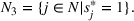
We now describe how our algorithms can be applied to solve the dynamic problems P1N‐D and P2N‐D using a rolling horizon strategy. In reality, the decision‐maker only knows the orders that have arrived and has no information about future order arrivals. Thus, to apply our algorithms in a dynamic setting, the problem we solve in each rolling horizon consists of the orders that have arrived only. Specifically, we first partition the planning horizon T into E equal‐length decision epochs, each represented by a time interval [(e − 1)δ, eδ], for e = 1, …, E, where δ = T/E denotes the length of each epoch. Let N_e denote the set of orders to be fulfilled in epoch e, that is, N_e = {j ∈ N | (e − 1)δ < d_j ≤ eδ}. The static problem to be solved for each epoch e (1 ≤ e ≤ E) consists of the orders in N_e, and this problem is solved in interval [(e − 1)δ – ρ, (e − 1)δ], where ρ is the allowed computational time. We note that ρ is a relatively small value compared to δ, and E is chosen such that ρ + δ ≤ L. Clearly, all the orders in N_e have arrived by the time (e − 1)δ – ρ and hence are known to the decision‐maker before the static problem for epoch e is solved. In fact, in addition to the orders in N_e, there are possibly some other orders that have arrived by the time (e − 1)δ – ρ. Those orders are not included in N_e because their pickup ready times are later than eδ and hence do not need to be considered in epoch e. Let

$N_e^{\prime }$

denote the set of such orders, that is,

$N_e^{\prime }$

= {j ∈ N | a_j ≤ (e − 1)δ – ρ, d_j > eδ}. The orders in

$N_e^{\prime }$

will be considered in the next decision epoch, along with some other orders. Figure 2 illustrates how the rolling horizon strategy works. Let P1N‐D(e) denote the fulfillment scheduling problem for epoch e when store fulfillment is not allowed, and P2N‐D(e) that when store fulfillment is allowed. We note that, different from P2N‐D, we restrict that in P2N‐D(e) orders fulfilled at the store must be processed within epoch e (i.e., within interval [(e − 1)δ, eδ]). It is clear that each problem P1N‐D(e) (respectively P2N‐D(e)) can be easily transformed into problem P1N (respectively P2N).

FIGURE 2

The rolling horizon strategy

In our experiments, we set u = 6 and randomly select d_j ∈ {2, 4, 6, 8, 10, 12} hours from time 0 for each j ∈ N. When implementing the rolling horizon strategy, we set δ = 3 hours (i.e., E = 4), ρ = 10 minutes, and solve each P1N‐D(e) and P2N‐D(e) using heuristics H1‐LS and H3‐LS, respectively. For each problem of P1N‐D and P2N‐D, we test n ∈ {200, 300, 500}, k ∈ {2, 4, 6}, and α ∈ {5, 10}. The remaining parameters are generated the same way as in Section 6.1. We generate 10 random instances for each combination of (n, k) and α. For each instance, we calculate the relative cost gap R of our algorithms applied with the above described rolling‐horizon strategy compared to the lower bound, defined as R = (F^H − F^LB)/F^LB × 100%, where F^H is the total fulfillment cost of the schedule obtained by H1 (respectively H3) for P1N‐D (respectively P2N‐D) conducted under the rolling‐horizon strategy, and F^LB the lower bound of the optimal objective value of P1N‐D and P2N‐D obtained by Algorithm A‐D (respectively DP‐D) given in Appendix A7 (Supporting Information). We note that Algorithms A‐D and DP‐D are designed under the assumption that all the future orders are known in advance at time 0. Thus, the lower bounds F^LB used here are generally not tight. We report in Table 6 the average (respectively maximum) value of R for each (n, k) and α under columns “R_avg” (respectively “R_max”) for both problems P1N‐D and P2N‐D.

TABLE 6

The performance of our algorithms under the dynamic setting

	P1N‐D				P2N‐D
	α = 5		α = 10		α = 5		α = 10
(n, k)	R avg	R max	R avg	R max	R avg	R max	R avg	R max
(200, 2)	15.5	26.13	14.65	25	5.17	8.81	5.49	8.72
(200, 4)	12.26	18.4	11.45	17.14	7.87	18.25	7.09	15.03
(200, 6)	13.75	18.54	11.65	17.4	6.98	18.46	6.38	14.53
(300, 2)	8.5	12.2	8.47	12.3	2.04	4.02	2.56	4.01
(300, 4)	8.37	12.42	7.84	12.35	4.33	7.77	4.18	5.45
(300, 6)	11.61	16.5	10.19	13.21	5.53	8.38	4.96	6.6
(500, 2)	4.51	7.1	4.61	7.01	1.24	3.17	1.56	2.9
(500, 4)	5.76	7.21	5.54	7.1	1.2	3.89	1.47	4.08
(500, 6)	5.04	9.85	4.76	8.21	1.43	4.81	1.69	4.53
Average	9.48	14.26	8.8	13.3	3.98	8.62	3.93	7.32

From Table 6, we can see that our algorithms implemented in a rolling horizon fashion perform well when used to solve the dynamic problems, even relative to fairly loose lower bounds. Specifically, the average cost gaps of the algorithms for the tested problem scales vary from 1.2% to 15.5% with most below 10%. In addition, we can observe that as order volume increases, the performance of our algorithms applied in the dynamic setting is also significantly improved. This is because when the order volume is small, knowing full information of the orders, as in Algorithms A‐D and DP‐D used to generate lower bounds, can take advantage of order batching opportunities to achieve lower costs. However, when the order volume is large, such benefit of order batching is less significant.

CONCLUSIONS AND EXTENSIONS

We have studied two fulfillment scheduling problems involving BOPS orders by clarifying the computational complexity of the problems, developing exact and heuristic algorithms, and analyzing the performance of the heuristics. The heuristics are shown to perform well, particularly for large problem instances. We have also generated some important managerial insights about BOPS order fulfillment.

Four extensions to our problems have been studied in the appendices. First, in the problems studied in the previous sections, the fixed cost for using a prescheduled truck is identical (which is α) and independent of the spare capacity of the truck. We can extend these problems to a more general setting where the fixed cost is truck dependent, that is, the fixed cost for using one prescheduled truck may be different from that of another prescheduled truck. We show that under this more general setting, the splittable problem P1S becomes ordinarily NP‐hard even with a fixed k, by first proving it is at least ordinarily NP‐hard, and then proposing a pseudo‐polynomial time algorithm for solving the problem. These results are given in Appendix A3 (Supporting Information). Similarly, we can show that problem P2S under this more general setting is also ordinarily NP‐hard even with a fixed k. It will be interesting to see how our heuristics perform for problems P1N and P2N under such a setting. Second, in Appendix A4 (Supporting Information), we consider an extension of problem P2 where there is an inventory availability constraint such that some orders in N are only available at the FC, some are only available at the store, and the rest are available at both the FC and the store. We show in Appendix 4 (Supporting Information) how the optimal algorithms (i.e., Algorithms A2 and DP1) developed for P2S and the heuristics proposed for P2N (i.e., heuristics H2 and H3) can be extended to solve the corresponding extensions, with the same theoretical performance guarantees. Third, in Appendix A5 (Supporting Information), we consider an extension of both problems P1 and P2 where there is a limited number of additional trucks available. This corresponds to the situation where the retailer has to predetermine the number of additional trucks to hire from 3PL based on the forecast before planning the order fulfillment operations. We show in Appendix A5 (Supporting Information) how the optimal algorithms (i.e., Algorithm A1, A2, and DP1) developed for P1S and P2S can be extended to solve their corresponding extension problems optimally, and how the heuristics (i.e., heuristics H1–H3) proposed for P1N and P2N can be extended to solve their corresponding extension problems with the same performance guarantees. Finally, in Appendix A6 (Supporting Information), we consider an extension of both problems P1 and P2 where there are multiple types of additional trucks that can be hired from 3PL such that different types of additional trucks have different capacities and different fixed costs. We investigate the complexity of various cases of the problems under this setting. It will be interesting to see whether our heuristics for P1N and P2N can be extended to such a setting with similar theoretical performance guarantees.

There are several possible topics for future research. First, as discussed in Section 5.2, it is an open question whether problem P2S with an arbitrary k is polynomially solvable or NP‐hard in the ordinary sense. Second, in the problems studied, there is a single store where all the BOPS orders are picked up by the customers. We can consider a setting where there are multiple stores, each owning a subset of BOPS orders, and the stores are located in the same neighborhood or same district of a city such that the transportation time and cost of a delivery trip from the FC to m stores are no more than those of a delivery trip from the FC to any single store. In such a setting, we do not need to consider routing issues, just as in the problems we have studied. We believe that extending our problems to such a more general setting makes the problems more difficult to solve, but expect that many of the results developed in this paper can be generalized to solve the same problems in this new setting.