Sage Journals: Discover world-class research

Abstract

Firms that sell products over a limited selling season often have only imperfect information about (a) the exact timing of that season, (b) the demand volume to expect, and (c) the temporal distribution of demand over the selling season. Given these uncertainties, firms must determine not only how much inventory to stock but also when to make that inventory available to customers. We thus ask: What is a firm's optimal inventory quantity and timing for products sold during a stochastic selling season? Although the newsvendor literature has developed a thorough understanding of the firm's optimal inventory quantity, it has failed to inform decision‐makers about choosing the optimal inventory timing. We address this issue by developing a theoretical model of a firm that sells a product over a stochastic selling season, and we study how this firm should choose its inventory timing and inventory quantity so as to maximize expected profits. We also identify the effects of optimal inventory timing on the firm's ability to satisfy customer demand and show how early inventory timing can be detrimental to customer service. Our core results imply three immediate recommendations for managers. First, optimal inventory timing is an effective weapon for combating both high inventory holding costs and high levels of uncertainty in the firm's customer demand pattern. Second, to be effective, a firm's inventory timing must be carefully aligned with the firm's inventory quantity. Third, naïve decision rules (e.g., “earlier is better”) may reduce not only the firm's profits but also its capacity to serve customer demand.

Keywords

demand timing demand uncertainty inventory management newsvendor seasonal product

INTRODUCTION

Inventory management of crop protection chemicals (e.g., fungicides, herbicides, and insecticides) shares many of the challenges associated with a classic newsvendor setting: (i) strong seasonal demand, (ii) considerable demand uncertainty, and (iii) long production lead times. Most crop protection chemicals are targeted at a particular phase of the crops' maturation process and can therefore be applied only a few weeks each year (see, e.g., Sainz Rozas et al., 2004; Vetsch & Randall, 2004). In addition, the type of chemicals that farmers must apply to their fields—as well as how much of them and when—depends heavily on that season's weather conditions (Caseley, 1983; Frey et al., 1973; Van Alphen & Stoorvogel, 2002). Hence farmers postpone the acquisition of their crop‐protecting chemicals until they can predict, with sufficient precision, such factors as sunshine and precipitation levels; thus the chemicals in question are not purchased until shortly before their application. Exacerbating the uncertainty is that fluctuating crop prices and changing environmental policies can have a sizable effect on farmers' incentives to invest (or not) in yield‐enhancing crop treatment (see, e.g., Böcker & Finger, 2017, and the references therein). Overall, then, agrochemical manufacturers face significant demand uncertainty and so are confronted with challenging inventory decisions. Complicating the problem further is that production processes for crop protection chemicals are, like those for pharmaceuticals, complex and time consuming: the total lead time of active ingredient synthesis, product formulation, and product distribution can run as long as 18 months (Comhaire & Papier, 2015; Shah, 2005). It follows that agrochemical manufacturers must make their inventory decisions well ahead of their products' selling seasons.

Given the foregoing description of the agrochemical market (and the properties of crop protection chemicals), one might be tempted to derive optimal inventory policies by applying the classic newsvendor model. Upon closer inspection of the setting, however, it is evident that two assumptions of that model severely limit its applicability in this context—similar limitations can be found for other products whose sales follow climatic seasons and that must be preproduced (e.g., lawn and gardening items, sun care products, and nonfood specials at discount retailers). First, the newsvendor model assumes that demand materializes at a single moment in time; thus it abstracts from the extended period of time characteristic of many selling seasons. In doing so, the model ignores that customer demand may change over time—for instance, there might be little demand at the start of the selling season but strong demand at the end (or vice versa). Accounting for the customer demand pattern becomes relevant when a firm is confronted with nonnegligible costs of holding inventory, as is the case for agrochemical manufacturers. In the agrochemical industry, contribution margins can differ widely across products; and while inventory holding costs may only have a minor impact on the profitability of high‐margin products, the impact is substantial for low‐margin products. For instance, holding a product with a gross margin of 20% for 3 months even at a moderate monthly holding cost rate of 1% erases a significant share of that product's financial potential. For other products, the situation is even worse: toxicity and special storage requirements can lead to much higher inventory holding cost rates.

Second, and even more problematic, the classic newsvendor model assumes that firms have perfect information about the timing of customer demand—in other words, it assumes that the demand timing is deterministic. As a result, the newsvendor model yields a simple inventory timing criterion: inventory should be made available just before demand occurs. However, this simplistic rule does not work for products with climatic seasons as, for instance, in the agrochemical market. Because farmers adjust their purchase of crop‐protecting chemicals in response to a number of erratic factors—including weather conditions as well as (volatile) crop prices—the timing of their demand is uncertain from the vendor's perspective; hence agrochemical manufacturers must make their inventory decisions in the context of great uncertainty regarding demand timing and quantity (Bouma, 2003; Teasdale & Shirley, 1998). In order to manage these uncertainties proactively, firms must carefully choose not only their inventory quantity but also their inventory timing. Deriving the optimal inventory quantity and timing and studying the interaction effects between these two decisions are the aims of our study.

As for inventory timing, agrochemical manufacturers could place a safe bet and decide to have next season's inventory ready immediately after the previous season ends. Yet such an inventory policy is economically infeasible: manufacturers would incur prohibitive inventory holding costs because items would be held in stock for many months without a single purchase. Also, because of highly complex production processes, classic quick‐response strategies in the spirit of Fisher et al. (2001) can hardly be applied in this context either. To save on holding costs, firms must therefore choose an inventory timing that is much closer to the expected start of the selling season; however, the later their inventory becomes available, the higher is the risk of early customer demand not being satisfied. So in their choice of inventory timing, firms must strike a balance between reducing their holding costs and increasing their risk of unserved demand. Naturally, this trade‐off also has immediate implications for a product's optimal inventory quantity.

The extant literature on inventory management for products with a limited selling season has more than adequately addressed the topic of how best to choose an optimal inventory quantity (see, e.g., Arrow et al., 1951; Cachon & Kök, 2007; Silver et al., 2017; Song et al., 2020). Yet it has failed to inform decision‐makers about how to choose the optimal inventory timing, especially in the case of a stochastic selling season, and neither has it discussed the interaction effects between a firm's inventory timing and quantity decisions. We seek to fill this research gap by developing a stylized model that captures the basic trade‐offs underlying the firm's inventory timing and inventory quantity decision. In short, our model enables a systematic study of the firm's optimal inventory policy.

Our contributions

The theoretical model we develop yields two novel insights concerning the management of inventories of products for which there is a limited (and stochastic) selling season.

First, we characterize an optimal inventory policy by deriving the firm's optimal inventory timing and also its optimal inventory quantity. We find that the latter reflects a timing‐adjusted critical fractile solution, whereas the former depends on (a) the expected customer demand pattern and (b) the hazard rate of the season's starting time. In addition, our results identify a nontrivial interaction between the firm's quantity and timing decisions. We also show how a firm can use its inventory timing to manage inventory holding costs; thus the firm, in essence, uses its timing decision to “steer” the effective profit margin of its products. It is this endogenization of profit margins that allows the firm to sell its products profitably even when faced with significant holding costs and highly uncertain demand. We also quantify the effect of an optimal inventory timing on a product's profitability by conducting a numerical analysis for a realistic range of parameters: we find that optimal inventory timing increases expected gross margins by

1 -- 2 %

, on average, but that it can lead to an increase of

9 -- 10 %

for low‐margin products.

Second, we disentangle the performance implications of an optimally chosen inventory timing. More specifically, we identify the conditions under which, with a later inventory timing, the firm not only increases its profits but also improves customer service—even though the risk of missing early season demand increases. The reason for this rather surprising result is the existence of subtle interaction effects between the firm's inventory timing and quantity decisions. With a later inventory timing, the firm increases (decreases) its effective underage (overage) costs because it saves on inventory holding costs; this altered cost structure may lead the firm to stock more items and thereby allow it to satisfy more demand. Our analysis reveals that this interaction effect is most prominent when inventory holding costs and demand uncertainty are significant.

Our main insights suggest a set of key managerial guidelines. First, the findings presented here underscore that managers should choose their inventory timing carefully. Being overly hasty and always offering inventories early on is not necessarily a wise strategy; in fact, such a naïve decision rule may well reduce profits as well as customer service. Second, managers should realize that their inventory timing flexibility is an effective tool with which to combat high inventory holding costs and high levels of uncertainty about customer demand patterns. It is ultimately a product's inventory timing that determines whether or not that product will be profitably sold. Last, managers should carefully align their inventory quantity and timing decisions and thus consider them jointly in their planning process.

Related literature

Inventory management for products that have uncertain customer demand patterns is a topic of long‐standing academic interest (Arrow et al., 1951; Petruzzi & Dada, 1999; Ravindran, 1972; Silver et al., 2017; Whitin, 1955). The central question addressed by this stream of literature is as follows: How much inventory should be stocked so that uncertain future customer demand is best satisfied? Given the importance of this question for virtually every product, scholars have devised a wide range of answers regarding many different product and market environments; for an excellent overview of the extant research, see Axsäter (2015). Most closely related to our work is the classic newsvendor literature on inventory management for products with a limited selling season. In essence, that model characterizes the optimal inventory quantity for a firm selling a single product with probabilistic demand over a single selling season (Porteus, 1990). This model has been extended to enhance its practical applicability by incorporating additional pricing decisions (Cachon & Kök, 2007; Petruzzi & Dada, 1999; Raz & Porteus, 2006; Salinger & Ampudia, 2011), different risk attitudes (Chen et al., 2009; Eeckhoudt et al., 1995), varying degrees of demand information (Ben‐Tal et al., 2013; Perakis & Roels, 2008), the benefits of quick‐response strategies (Cachon & Swinney, 2011; Iyer & Bergen, 1997; Milner & Kouvelis, 2005), and the impact of different inventory financing options (Gaur & Seshadri, 2005; Kouvelis & Zhao, 2012).

The extension with the greatest bearing on our study examines the value of postponing production in a newsvendor context (e.g., Anupindi & Jiang, 2008; Iyer et al., 2003; Ülkü et al., 2005; Van Mieghem & Dada, 1999). This stream of literature studies the optimal starting time for a firm's inventory production, with a later production leading to more accurate demand forecasts yet also to higher production costs. Research has extended initial findings to discuss the applicability of different mechanisms for updating demand forecasts (Boyaci & Özer, 2010; Oh & Özer, 2013; T. Wang et al., 2012), the role of production lead times (Y. Wang & Tomlin, 2009), and the impact of multiple sales opportunities (Song & Zipkin, 2012). We concur with these papers' argument that a firm's production (or inventory) timing is a critical decision for effective inventory management; however, we extend—and complement—previous research by analyzing a practically relevant yet overlooked trade‐off. In particular, the primary reason for a later inventory timing may not always be the acquisition of more precise demand information; rather, such timing serves as a tool for reducing high inventory holding costs while hedging against uncertainty in the demand pattern of customers. Of course, a firm's cost structure also interacts with the firm's ability to wait for advanced demand information: reduced inventory holding costs allow the firm to wait longer for more precise demand information, and once obtained, this advanced information can then be used to lower inventory holding costs even further.

Finally, our contribution can be viewed from the perspective of research on (random) product obsolescence and its effects on a firm's optimal inventory quantity. Initiated by the pioneering work of Hadley and Whitin (1961), Hadley (1962), and Hadley and Whitin (1962) and later extended by Pierskalla (1969), Nahmias (1977, 1982), and Song and Zipkin (1996), this literature addresses the optimal inventory quantity for a firm that must balance its inventory holding costs with the risks originating from a stochastic selling season. We follow this stream of work by investigating how inventory holding costs affect a firm's optimal inventory policy when the firm's selling season is stochastic. However, we depart from this literature by allowing the firm to choose its inventory timing endogenously. Because the papers cited here all assume that a firm's inventory timing is exogenous, they ignore the effects of holding costs or a stochastic selling season on a firm's inventory timing decision.

The paper is organized as follows. We introduce our theoretical model in Section 2 before we derive the firm's optimal inventory policy in Section 3. We then study how varying customer demand patterns affect the firm's optimal inventory policy (Section 4), and we provide a numerical study that quantifies the benefits of an optimal inventory timing (Section 5). Section 6 summarizes our results and discusses some limitations of our analysis. All proofs are relegated to Appendix A.

MODEL SETUP

We base our model of a firm with a stochastic selling season on the fundamentals of the classic newsvendor model. Thus, we consider a firm that sells a single product over a limited selling season and that must decide on an inventory policy well before the season starts. So, when selecting its inventory policy, the firm has imperfect information about customer demand—in terms of the product's demand volume and the exact shape and timing of the customer demand pattern. Once production is completed and the firm's inventory becomes available, the firm can use that inventory to satisfy customer demand; yet the firm also incurs inventory holding costs until the inventory is either depleted or salvaged. The salvaging of all unsold items occurs at the end of the selling season when customer demand has ceased. The rest of this section details our model setup and assumptions.

Inventory policy and stochastic selling season

The classic newsvendor model—the starting point of our theoretical model—is useful for firms that are confronted with stochastic demand over a finite selling season and that must make a single inventory quantity decision before the start of their selling season. As discussed in Section 1, those assumptions approximate the reality in our motivating example, the agrochemical industry, reasonably well. In particular, in the agrochemical industry, demand is clearly uncertain and seasonal. Moreover, due to complex production processes and a global supply chain structure, production lead times are long, which severely limits an agrochemical manufacturer's ability to adjust inventory quantities close to the selling season. Furthermore, significant setup costs prevent agrochemical manufacturers from spreading production over time; thus while the details of the production process are of course more complex, the assumption of a single‐order opportunity captures the essence of a manufacturer's limited flexibility rather well.

Those commonalities notwithstanding, the classic newsvendor model also exhibits a major shortcoming: it ignores the possibility of a stochastic selling season, which is a key issue in the agrochemical industry. To account for the peculiarities of a stochastic selling season, we extend the classic newsvendor model along two dimensions. First, besides deciding on the inventory quantity x—the standard decision variable in newsvendor contexts—we allow the firm also to choose its inventory timing t; that is, by choosing t the firm decides on the earliest time its inventory can be used to satisfy customer demand. An earlier inventory timing likely allows the firm to capture a larger portion of customer demand, but this advantage comes at the expense of an extended period of holding inventory and thus higher holding costs. Throughout the analysis, we measure time

τ \geq 0

continuously and refer to the pair

(x, t)

as the firm's inventory policy, which must be fixed before time

τ = 0

Second, we depart from previous work by considering stochasticity in the product's selling season (i.e., in the shape and timing of the customer demand pattern), and not just the product's demand volume

Q \geq 0

. Three statistics are needed for a full characterization of the selling season's properties: (i) the beginning B of the season; (ii) the length L of the season; and (iii) the shape

A (τ; Q, B, L)

of the customer demand pattern over the season, where

A (τ; Q, B, L)

measures the portion of demand that becomes manifest after time τ for given values of Q, B, and L. With these definitions in hand, we can write future demand at time τ—that is, the demand that arises after time τ—as

Q (τ) = Q A (τ; Q, B, L)

We assume that customer demand occurs only within the selling season and that unserved customers are lost. The mathematical implication is that, for any given Q, B, and L,

A (τ; Q, B, L)

must satisfy these three properties: (i)

A (τ; Q, B, L) = 1

for all

τ \leq B

, (ii)

A (τ; Q, B, L) = 0

for all

τ \geq B + L

, and (iii)

A (τ; Q, B, L)

is decreasing for all other τ. We further assume that, for any realization of Q, B, and L,

A (τ; Q, B, L)

is a deterministic function of τ, and it is once continuously differentiable in τ. We can then express, for any given Q, B, and L, the customer demand rate at time τ as

D (τ) = - Q A^{'} (τ; Q, B, L) \geq 0

, where

A^{'} (τ)

denotes the derivative of

A (τ)

with respect to τ. In addition, we assume that B and L are continuous random variables with support on

[0, b_{u}]

and

(0, l_{u}]

, respectively; here

b_{u} \geq 0

and

l_{u} > 0

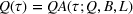
Figure 1 illustrates the relationships among a product's demand volume, the properties of its selling season, and the firm's inventory policy: in the left panel, the firm's inventory timing occurs prior to the beginning of the selling season (i.e.,

t < B

) and the inventory quantity is insufficient to satisfy all the demand (i.e.,

x < Q

). In contrast, the right panel shows a setting in which the firm's inventory becomes available only after the season has already started (i.e.,

t > B

) and there are—at the end of the season—unsold items that the firm must salvage (i.e.,

x > Q (t)

). It is a vital feature of our model—and a challenging empirical reality—that imperfect information about customer demand prevents the firm from exactly synchronizing its inventory policy with the true customer demand pattern.

FIGURE 1

Inventory policy and customer demand pattern

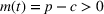
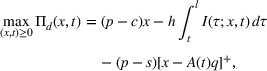
The firm's optimization problem

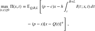
The firm's goal is to maximize its profits. As in the classic newsvendor model, the firm incurs a per‐unit production cost

c > 0

, realizes a price

p > c

per unit sold, and salvages any unsold item at

s < c

when the selling season ends. In addition, the firm incurs holding costs. Inventory occurs because (a) the firm seeks to satisfy demand over a nonnegligible portion of the length L of the selling season and (b) it cannot perfectly predict the beginning B of the selling season. We capture inventory holding costs as follows: starting with the availability of inventory at time t, the firm incurs holding costs

h \geq 0

per unit of inventory and time until the inventory is either depleted or salvaged. Note that we do not allow the firm to salvage items during the selling season. This assumption is but mildly restrictive: because production costs c are already sunk, the decision whether (or not) to salvage an item during the selling season is solely based on the benefits of salvaging versus the firm's prospective sales revenues—and not profit margins. And in reality, firms rarely find it optimal to sacrifice future sales revenues to save some holding costs by salvaging.

Taken together, these considerations require the firm to choose an inventory policy

(x^{*}, t^{*})

that maximizes its expected profits: sales revenue minus the costs of production, inventory holding, and salvage. Thus the firm's optimization problem is

\begin{matrix} \max_{(x, t) \geq 0} Π (x, t) & = & E_{Q, B, L} [(p - c) x - h \int_{t}^{B + L} I (τ; x, t) d τ \\ - (p - s) {[x - Q (t)]}^{+}], \end{matrix}

1where

I (τ; x, t) = {[x - (Q (t) - Q (τ))]}^{+}

denotes the firm's inventory position at time

τ \in [t, B + L]

for a given inventory policy

(x, t)

, and

{[Z]}^{+} = \max {0, Z}

. Figure 1 visualizes how

I (τ; x, t)

changes over the course of a selling season.

SERVING A STOCHASTIC SEASON

We now study the properties of a firm's optimal inventory policy. We begin by formally deriving the firm's optimal inventory quantity and timing (Section 3.1). Then we investigate how those optimal decisions interact and evaluate how the chosen inventory policy affects the firm's ability to satisfy customer demand (Section 3.2).

The optimal inventory policy

To better disentangle the different forces at play, we derive the firm's optimal inventory policy in two steps. First, we characterize the firm's optimal inventory quantity

x^{*} (t)

for a given inventory timing t. We then determine the optimal inventory timing

t^{*}

, taking into account the dependence of

x^{*} (t)

on t. Proposition 1

For given

t \geq 0

, let

m (t)

be the expected profit margin of the first sold item; that is,

m (t) = p - c - h \int_{t}^{b_{u}} P (B > b) d b

t \in [0, b_{u}]

m (t) = p - c

t \in (b_{u}, b_{u} + l_{u}]

, and

m (t) = 0

otherwise. For a fixed inventory timing t, the optimal inventory quantity

x^{*} (t)

is determined uniquely as a function of t:

(i)

for any t such that

m (t) \leq 0

x^{*} (t) = 0;

(ii)

for any t such that

m (t) > 0

x^{*} (t)

solves

\begin{matrix} P (Q (t) & \leq & x^{*} (t)) \\ = & \frac{p - c - h [\begin{matrix} \int_{t}^{b_{u}} P (B > b) d b + E_{B, L} [\int_{\max {t, B}}^{B + L} \\ P (Q (t) - Q (τ) \leq x^{*} (t) ∣ B, L) d τ] \end{matrix}]}{p - s} \\ = & \frac{m (t)}{p - s} - \frac{h}{p - s} E_{B, L} \\ \times [\int_{\max {t, B}}^{B + L} P (Q (t) - Q (τ) \leq x^{*} (t) ∣ B, L) d τ] . \end{matrix}

Moreover, (a)

P (Q (t) \leq x^{*} (t)) = (p - c) / (p - s)

h = 0

and (b)

0 \leq {(m (t) - h l_{u})}^{+} / (p - s) \leq P (Q (t) \leq x^{*} (t)) \leq m (t) / (p - s)

The proposition shows, in line with prior work on the newsvendor problem (see, e.g., Cachon & Kök, 2007; Petruzzi & Dada, 2010), that the optimal inventory quantity

x^{*} (t)

is determined by a “critical fractile” condition; hence, the firm sets a target service level for future demand

Q (t)

. In fact, in the absence of inventory holding costs (i.e., if

h = 0

), the critical fractile collapses to the classic newsvendor fractile (see part (a) of the proposition). In general, however, the critical fractile condition (2) differs from the classic newsvendor solution in two important ways. First, the critical fractile applies to the distribution of future demand

Q (t)

rather than total demand Q. The relevant demand distribution that the firm should consider when choosing its inventory quantity is thus dependent on the firm's inventory timing decision. Second, the product's profit margin is adjusted for inventory holding costs. In particular, incurred holding costs consist of two components (as reflected by the two integrals in (2)): the first integral accounts for the firm's expected marginal preseason holding costs, whereas the second integral captures the expected marginal in‐season holding costs. It is obvious that both terms are affected by the firm's inventory timing t; yet, marginal in‐season holding costs also depend on the firm's inventory quantity. As a result, the firm's optimal target service level (i.e., its critical fractile) is—even for a given inventory timing t—not exogenous to its inventory quantity decision. The final statement in Proposition 1 provides an exogenous upper and lower bound for the firm's target service level; those bounds are obtained from bounding the firm's expected in‐season holding costs.

As in the classic newsvendor model, the firm's optimal inventory quantity increases with the product's sales price p and salvage value s but decreases with the production cost c. More important for our work, however, is the effect of the firm's inventory holding costs h on

x^{*} (t)

: for a given inventory timing t, the optimal inventory quantity declines when h increases. The impact of h depends on the start and the length of the selling season but also on the shape

Q (τ)

of the customer demand pattern: if most demand manifests early in the season then in‐season holding costs are relatively small and thus have only a minor effect on

x^{*} (t)

; but if there are high levels of demand toward the end of the selling season, then in‐season holding costs can be substantial and so may induce the firm to choose a markedly lower inventory quantity.

Proposition 1 reveals that the firm's inventory timing affects the optimal inventory quantity in two distinct ways: namely by (a) determining the addressable portion of demand

Q (t)

and (b) by influencing—through inventory holding costs—the product's unit profit margin. The impact of the latter effect is represented by the function

m (t)

; it designates, for a given inventory timing t, the expected profit margin of the first sold item. Note that any further item has a lower expected profit margin because in‐season holding costs accumulate over time. Of course, if

m (t) \leq 0

, then selling the product would make no economic sense; hence

x^{*} (t) = 0

, as in part (i) of Proposition 1. However, by increasing t, the firm can save preseason holding costs and thus increase

m (t)

. In fact, a firm that chooses an inventory timing

t \in [b_{u}, b_{u} + l_{u}]

can avoid all preseason holding costs and realize the maximum attainable unit margin of

m (t) = p - c > 0

; that is, the firm can always select an inventory timing t such that

m (t) > 0

. It then follows from Proposition 1(ii) that the firm always finds it optimal to offer the product and that the optimal inventory quantity

x^{*} (t)

will be uniquely determined by (2).

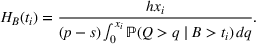
Equipped with these insights, we now turn to the firm's optimal inventory timing decision. To this end, we analyze how the firm selects its optimal inventory timing

t^{*}

by solving

\max_{t \geq 0} Π (x^{*} (t), t)

. This optimization problem is not quasi‐concave in t, in general, and as such it may—depending on the parameters of the problem—exhibit multiple local (or possibly even global) optima. Yet, this potential multiplicity of solutions does not affect any of our subsequent results. Proposition 2

The optimal inventory timing

t^{*}

satisfies the following necessary optimality condition:

\begin{matrix} h x^{*} (t^{*}) P (t^{*} & \leq & B + L) - h E_{B, L} [\int_{t^{*}}^{B + L} E_{Q} [D (t^{*}) ∣ Q (t^{*}) \\ - Q (τ) \leq x^{*} (t^{*}), B \leq t^{*}, L] P (Q (t^{*}) - Q (τ) \\ \leq & x^{*} (t^{*}), B \leq t^{*}) d τ] \\ = & (p - s) E_{Q, B, L} [D (t^{*}) ∣ Q (t^{*}) \leq x] P (Q (t^{*}) \\ \leq & x^{*} (t^{*})) . \end{matrix}

3Also,

t^{*} > 0

if and only if

h > 0

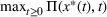
Two opposing effects determine the firm's optimal inventory timing. With a later inventory timing, the firm is able to reduce the time that items, which are sold later in the season, must be stored; the firm can hence reduce inventory holding costs. At the same time, however, the firm becomes more susceptible to losing demand early in the season; as a result, some items may need to be stored for a longer period of time until they are sold—if they are sold at all. Proposition 2 shows that the optimal inventory timing equates to the marginal impact of t on these effects. In particular, the left‐hand side of (3) characterizes the marginal change in expected holding costs when increasing t. Here, the first term captures the direct effect of reducing storage time, whereas the second term adjusts for the indirect effect that some items now need to be stored longer until they are sold. The right‐hand side represents the marginal increase in leftover inventory due to late inventory availability; those leftovers must be salvaged.

Proposition 2 also establishes that, as a consequence, choosing the earliest possible inventory timing (i.e.,

t = 0

) is optimal only in the absence of holding costs. In all other cases (i.e., if

h > 0

), the firm should trade off a (potentially small) risk of missing some early demand against reduced inventory holding costs. This is similar to the classic newsvendor logic, which prescribes that, in the presence of overage costs, a firm should accept a certain risk of losing sales.

Inventory timing and customer service

Because the firm's future demand volume

Q (t)

stochastically decreases with t, it would be natural to expect that a later inventory timing would result in stochastically less demand being satisfied. While this conjecture is obviously true for a fixed inventory quantity, we have learned from Proposition 1 that the firm should adjust its optimal inventory quantity as a function of t—this interdependence renders the impact of the firm's inventory timing on its service performance more intricate. In this section, we identify the conditions under which the above conjecture is (and is not) true.

As a starting point, we shed more light on the interaction between the firm's inventory timing t and the associated optimal inventory quantity

x^{*} (t)

. That is, how does

x^{*} (t)

change with t? Lemma 1

Let

f_{Y}

be the probability density function of the random variable Y. Then the firm's optimal inventory quantity

x^{*} (t)

increases with t if and only if

\begin{matrix} h P (t < B + L) - h E_{B, L} [\int_{t}^{B + L} E_{Q} [D (t) ∣ Q (t) - Q (τ) \\ \leq x^{*} (t), B \leq t, L] f_{Q (t) - Q (τ) ∣ B \leq t} (x^{*} (t)) P (B \leq t) d τ] \\ > (p - s) E_{Q, B, L} [D (t) ∣ Q (t) \leq x^{*} (t)] f_{Q (t)} (x^{*} (t)) . \end{matrix}

4In particular: (i) if

h = 0

then

x^{*} (t)

decreases with t, but (ii) if

h > 0

then there exists

\underset{̲}{t} > 0

such that

x^{*} (t)

increases with t for

t \in [0, \underset{̲}{t}]

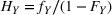
Lemma 1 provides a necessary and sufficient condition for

x^{*} (t)

to increase with the firm's inventory timing t. Despite its unwieldy appearance, condition (4) has an intuitive interpretation. Note that the critical fractile condition (2) stipulates two conditions under which

x^{*} (t)

increases with t: (i) the firm's expected underage costs must increase with t (which favors a higher

x^{*} (t)

); and (ii) this increase must be great enough to compensate for an expected reduction in future demand

Q (t)

(which favors a lower

x^{*} (t)

). Condition (4) formalizes this intuition. With a later inventory timing t, the firm reduces its expected unit holding costs (as given by the left‐hand side of (4)) and so increases its expected unit underage costs; if this holding cost reduction outweighs the additional loss in revenue (as given by the right‐hand side of (4)), then it is optimal for the firm to increase

x^{*} (t)

with t.

Parts (i) and (ii) of Lemma 1 provide further insights into the leading role that inventory holding costs play in the interaction between a firm's inventory quantity and timing decision. If there are no holding costs (

h = 0

), then the firm never benefits from simultaneously increasing its inventory timing and its inventory quantity. However, if inventory holding costs are strictly positive (

h > 0

), then the firm may benefit from increasing both decisions at the same time—but only if the customer demand rate

D (t)

is sufficiently small. The latter phenomenon typically occurs early in the firm's window of sales opportunity

[0, b_{u} + l_{u}]

: when

t \in [0, \underset{̲}{t}]

as in Lemma 1(ii).

As an aside, Lemma 1 also establishes an interesting interplay between demand uncertainty and the firm's optimal inventory quantity. Suppose that

t < t^{'}

; this inequality implies that

Q_{t}

first‐order stochastically dominates

Q_{t^{'}}

(i.e.,

P (Q_{t} \leq x) \leq P (Q_{t^{'}} \leq x)

for all

x \geq 0

). Lemma 1 now shows that first‐order stochastic dominance in demand does not always lead to higher inventory quantities—and so we may have

x^{*} (t^{'}) > x^{*} (t)

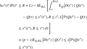
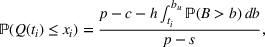
So far, we have established that the optimal inventory quantity may (or may not) increase with the firm's inventory timing. This finding allows us to examine the impact of the firm's inventory timing on its performance in terms of satisfying customer demand. In particular, will an earlier inventory timing always lead to a greater amount of satisfied demand, or equivalently, to a lesser amount of lost sales?

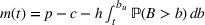
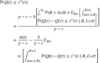
Note that lost sales in our setting occur for two different reasons: (i) demand occurs before the firm's inventory timing or (ii) the inventory quantity has been depleted. So for a given inventory policy

(x, t)

, the firm's expected lost sales are given by

L (x, t) = E_{Q, B, L} [(Q - Q (t)) + {[Q (t) - x]}^{+}]

. Given that

Q (t)

stochastically decreases with the firm's inventory timing t, it is obvious that expected lost sales increase with t if

x^{*} (t)

decreases with t. Yet by Lemma 1,

x^{*} (t)

may actually increase with t; in that event, expected lost sales may actually decrease with the firm's inventory timing. Our next proposition formalizes this intuition by giving necessary and sufficient conditions for

L (x^{*} (t), t)

to decrease with t. Proposition 3

L (x^{*} (t), t)

decreases with t if and only if

\begin{matrix} {(x^{*} (t))}^{'} > \frac{E_{Q, B, L} [D (t) ∣ Q (t) \leq x^{*} (t)] P (Q (t) \leq x^{*} (t))}{P (Q (t) > x^{*} (t))} . \end{matrix}

5In particular: (i) if

h = 0

then

L (x^{*} (t), t)

increases with t, but (ii) if

h > 0

then there exists

t_{l} > 0

such that

L (x^{*} (t), t)

decreases with t for

t \in [0, t_{l}]

The main outcome of Proposition 3 is that, in optimum, the firm's expected lost sales may decrease with its inventory timing—but only if inventory holding costs are sufficiently high. So if

h > 0

and if a later inventory timing is associated with a larger inventory quantity (per Lemma 1), then the increase in the optimal inventory quantity

{(x^{*} (t))}^{'}

may be larger than the increase in unsatisfied early demand (as given by the right‐hand side of (5)) and thereby lead to an overall reduction in expected lost sales.

From a managerial perspective, Proposition 3 falsifies the seemingly convincing argument that earlier inventory availability necessarily leads to a higher level of satisfied demand. In fact, a premature inventory timing may reduce a firm's capacity to satisfy demand because high inventory holding costs may force the firm to reduce its inventory quantity which, in turn, harms its service performance.

IMPACT OF CUSTOMER DEMAND PATTERN

The conditions that characterize the optimal inventory quantity and timing for a firm that faces a stochastic selling season are rather complex; this complexity is due to the interplay of several opposing forces (cf. Section 3.1). In this section, we aim to isolate some of those relevant effects to garner further insights by studying two special cases that are both instructive and practically relevant. In the first case, a firm is confronted with instantaneous demand; this setting allows us to isolate how uncertainty in demand timing (as captured by B) affects the firm's inventory timing (Section 4.1). In the second case, the firm has perfect information about the selling season's properties (Section 4.2); this analysis yields additional insights concerning the influence of varying demand patterns (as captured by

A (τ)

). Unless explicitly stated otherwise, we maintain the same modeling assumptions as in our base model.

Instantaneous demand

It is common in the newsvendor literature to abstract from the dynamics within the selling season and instead to assume that all demand occurs at a single and ex ante known moment in time (see, e.g., Choi, 2012; Petruzzi & Dada, 1999, 2010; Qin et al., 2011). Given that assumption, the firm's inventory timing is trivial: inventory should be made available just before demand occurs. In this section, we follow the assumption of instantaneous demand—that is, in our demand model, we set the season length to zero:

L = 0

and

A (τ; B) = 1_{{τ \leq B}}

—but depart from the traditional newsvendor setting by viewing the demand timing B as uncertain. In this setting, choosing an adequate inventory timing becomes a challenging task for the firm.

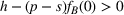
Despite its simplicity, the assumption of instantaneous demand is a reasonable approximation of the market structure in many real‐world scenarios. Thus instantaneous demand is a realistic assumption if (a) a firm's selling season is indeed short (e.g., only a few days) and/or (b) its in‐season holding costs are negligible (though preseason holding costs may still be important). Under those conditions, the firm's optimization problem (1) reduces to

\begin{matrix} \max_{(x, t) \geq 0} Π_{i} (x, t) & = & E_{Q, B} {[(p - c) x - h x [B - t]}^{+} \\ - (p - s) {[x - Q (t)]}^{+}] . \end{matrix}

6It is easy to see that when holding costs are negligible (i.e.,

h \approx 0

), then the firm finds it optimal to make its inventory available as early as possible (i.e., it would set

t_{i} = 0

). Instantaneous demand can hence induce a firm to choose

t_{i} = 0

even when

h > 0

, a decision that would be suboptimal for an extended selling season (cf. Proposition 2). In those cases, the promise of holding cost savings never outweighs the downside risk of losing the entire season's demand. However, when holding costs are sufficiently high, this argument is no longer correct: the firm should postpone its inventory timing. For the case of sufficiently high holding costs, we establish the firm's optimal inventory policy

(x_{i}, t_{i})

—that is, the solution to (6)—in Proposition 4. Proposition 4

Assume that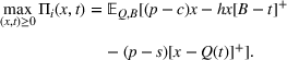

h - (p - s) f_{B} (0) > 0

, and let

H_{Y} = f_{Y} / (1 - F_{Y})

denote the hazard rate of the random variable Y, with

F_{Y}

being the cumulative distribution function of Y. Then, the firm's optimal inventory policy solves

\begin{matrix} P (Q (t_{i}) \leq x_{i}) = \frac{p - c - h \int_{t_{i}}^{b_{u}} P (B > b) d b}{p - s}, \end{matrix}

\begin{matrix} H_{B} (t_{i}) = \frac{h x_{i}}{(p - s) \int_{0}^{x_{i}} P (Q > q ∣ B > t_{i}) d q} . \end{matrix}

8Furthermore,

H_{B}^{'} (t_{i}) \geq 0

As in our base model, the firm's optimal inventory quantity is determined by a critical fractile condition on

Q (t_{i})

; thus the only difference between (7) and (2) is that the former does not include an adjustment term for in‐season holding costs. It is also interesting to note that even in the absence of in‐season holding costs, the optimal inventory quantity

x_{i}

is smaller than in classic newsvendor settings—this is due to the (preseason) holding costs incurred until the (uncertain) start of the season.

There is an appreciable reduction in complexity when comparing the firm's inventory timing under instantaneous demand (as given by (8)) with our base case of a finite season length (as given by (3)). Here, the firm's optimal inventory timing is determined by a simple hazard rate condition that balances the firm's earliness/holding costs with its tardiness costs (i.e., expected lost revenues). In particular, the firm should choose its inventory timing such that, at

τ = t_{i}

, the likelihood of demand occurrence—given that demand has not materialized earlier—equates to a predefined threshold.

According to Proposition 4, a firm's optimal inventory timing

t_{i}

is determined by the hazard rate of demand timing (i.e., by

H_{B}

). In particular, the more rapidly the likelihood of demand occurrence increases over time, the earlier the firm should make its inventory available; and ceteris paribus,

t_{i}

increases with h and s but decreases with p because

H_{B}^{'} (t_{i}) \geq 0

. This finding suggests that when holding inventory becomes more expensive relative to the revenue difference between regular sales and salvaging (i.e., if

h / (p - s)

increases), firms should accept a higher risk of missing an early season. Even though this strategy may lead to less items being sold, in expectation, it allows the firm to sell items at higher margins.

Deterministic selling season

In this section, we study more closely how the properties of

A (τ)

affect the firm's inventory timing. For this purpose, we consider a deterministic analogue of our base model by assuming that all characteristics of the selling season are perfectly known. Thus, we set

Q = q > 0

B = 0

, and

L = l > 0

while assuming that

A (τ)

is given. Then the deterministic analogue of the firm's profit function (1) can be written as

\begin{matrix} \max_{(x, t) \geq 0} Π_{d} (x, t) & = & (p - c) x - h \int_{t}^{l} I (τ; x, t) d τ \\ - (p - s) {[x - A (t) q]}^{+}, \end{matrix}

9and the optimal inventory policy

(x_{d}, t_{d})

is derived using Proposition 5. To simplify the analysis, we focus on those cases when inventory holding costs do not exceed the product's profit margin. Proposition 5

Assume that

p - c \geq h l

. Then, the firm's optimal inventory policy solves

\begin{matrix} x_{d} = A (t_{d}) q, \end{matrix}

\begin{matrix} - \frac{A^{'} (t_{d})}{A (t_{d})} = \frac{h}{p - c} . \end{matrix}

11Moreover, (i)

t_{d} = 0

if and only if

h = 0

, (ii)

A (τ)

is log‐concave at

τ = t_{d}

, and (iii)

t_{d}

(respectively

x_{d})

increases (respectively decreases) with h.

This proposition reveals that, for a deterministic selling season and moderate holding costs, the firm simply chooses its inventory quantity so as to satisfy all demand that occurs after the inventory timing (i.e.,

x_{d} = A (t_{d}) q

). It is intuitive that, since the firm can perfectly predict demand and since it is always profitable to sell the product, the firm is determined to serve every single customer once inventory is available. Yet this strategy does not imply that the firm makes its inventory available immediately; rather, the firm continues to trade off lost sales early in the season against reduced holding costs for serving later demand. Technically, the optimal inventory timing

t_{d}

is determined by the logarithmic derivative of

A (τ)

; that is, the firm selects its inventory timing such that, at

τ = t_{d}

, the ratio of demand rate over future demand meets a predefined target value. Also, because the firm is able to perfectly synchronize inventory with demand,

t_{d}

is independent of

x_{d}

and s. In particular, (11) establishes that—for the optimal inventory timing—the marginal loss of revenue from further postponing the product's availability must equal the firm's marginal holding costs.

An intriguing observation is that a firm's optimal inventory timing depends on the slope and curvature of

A (τ)

. This finding has two central managerial implications. First, it identifies—via Proposition 4—that there are two major factors that managers should consider when choosing their inventory timing: (i) the hazard rate of the season start B and (ii) the slope and curvature of the (expected) demand pattern

A (τ)

. Note that the optimal timing condition (3) in our base model is a convolution of those two components. In practice, relying on these two factors considerably reduces the managerial decision problem's complexity. Second, Proposition 5(iii) establishes that the firm—in response to an increase in holding costs—never increases both its inventory timing and inventory quantity if the selling season is deterministic. We can therefore conclude that the unexpected interaction effects described in Lemma 1 and Proposition 3 are mainly driven by the firm's lack of knowledge about the exact properties of its selling season.

QUANTIFYING THE IMPACT OF INVENTORY TIMING

Having characterized the main trade‐offs that the firm must balance with its inventory policy when serving a stochastic selling season, we now turn to the magnitude of the effects resulting from an optimally chosen inventory policy. Through an extensive numerical simulation, we investigate (a) whether (or not) inventory timing has a first‐order effect on firm profits and (b) how the firm's inventory policy and profits are affected by parameter changes.

Simulation setup and choice of parameters

To shed light on the influence of our various model parameters, we constructed our simulation study in a full factorial design over a wide range of parameter values, as listed in the leftmost column of Table 1. In total, we analyze 2187 different scenarios. The chosen parameter values reflect typical agrochemical products and their selling seasons, as discussed below.

TABLE 1

Results of numerical experiments

		h‐ $n v$ policy		Optimal policy
		$Δ Π_{avg}^{h - n v}$ (%)	$Δ Π_{0.95}^{h - n v}$ (%)	$Δ Π_{avg}^{*}$ (%)	$Δ Π_{0.95}^{*}$ (%)	$t^{*} / b_{u}$	$x_{n v} - x^{*}$
	25	0.01	0.05	0.16	0.59	0.13	0.74
c	50	0.05	0.26	0.64	2.30	0.18	1.10
	75	0.35	1.49	2.89	9.94	0.26	2.05
	0.01	0.02	0.09	0.41	1.94	0.16	0.50
ρ	0.02	0.10	0.52	1.13	5.14	0.19	1.29
	0.03	0.29	1.42	2.15	9.74	0.22	2.11
	10	0.04	0.23	0.91	4.22	0.18	0.46
σ	30	0.13	0.61	1.22	5.46	0.19	1.54
	50	0.24	1.19	1.57	7.11	0.21	1.90
	(1,1)	0.13	0.62	0.73	3.35	0.11	1.38
$(α, β)$	(2,4)	0.10	0.46	0.75	3.21	0.12	1.16
	(4,2)	0.17	0.82	2.21	9.07	0.35	1.35
	1	0.10	0.47	0.89	4.05	0.21	1.13
$b_{u}$	1.5	0.13	0.62	1.23	5.56	0.19	1.30
	2	0.17	0.83	1.57	7.37	0.18	1.46
	0.8	0.04	0.22	0.74	3.49	0.13	0.71
L	1.5	0.09	0.47	1.10	5.20	0.18	1.10
	3	0.28	1.42	1.85	8.98	0.27	2.08
	$\frac{Q}{L}$	0.14	0.65	0.95	4.50	0.14	1.34
$D (τ)$	$\frac{2 Q (τ - B)}{L^{2}}$	0.18	0.85	2.04	9.07	0.32	1.39
	$\frac{2 Q (B + L - τ)}{L^{2}}$	0.09	0.48	0.70	3.20	0.11	1.16
	Total	0.14	0.64	1.23	5.57	0.19	1.30

As for product characteristics, we account for the reality that agrochemical products differ widely in (a) their profit margins and (b) their inventory holding costs (e.g., because some products rely on more expensive raw materials than others or require special storage conditions). We represent products with different profit margins by fixing the sales price

p = $ 100

while varying production costs

c \in {$ 25, $ 50, $ 75}

. For simplicity, we normalize the salvage value to zero (

s = $ 0

). Inventory holding costs h are measured—as it is standard in practice—as percentage ρ of production costs (i.e.,

h = ρ c

); here

ρ \in {1 %, 2 %, 3 %}

per month (or equivalently,

12 -- 36 %

per year), which covers the full spectrum from common items (

ρ = 1 %

) to even the most hazardous materials (

ρ = 3 %

With respect to the characteristics of the selling season, we differentiate between a “near‐instantaneous” season (

L = 0.8

months), a moderate season (

L = 1.5

months), and a “climatic” season (

L = 3

months). The beginning B of the season can be more or less uncertain in reality: we capture this fact by (a) varying the support

[0, b_{u}]

of B, with

b_{u} \in {1, 1.5, 2}

(measured in months) and (b) changing the relative likelihood of an early versus a late season start. To this end, we assume

B \sim B 1 (b_{u}, α, β)

, with

B 1

being the beta distribution of the first kind (Donald & Xu, 1995), and

(α, β) \in {(1, 1), (2, 4), (4, 2)}

. In addition, agrochemical manufacturers also encounter varying customer demand patterns: whereas for some products customer demand is relatively constant over the course of a season, other products may experience time‐varying demand. In our simulation study, we examine the case of a constant (

D (τ) = Q / L

), an increasing (

D (τ) = 2 Q (τ - B) / L^{2}

), and a decreasing demand rate (

D (τ) = 2 Q (B + L - τ) / L^{2}

), with

τ \in [B, B + L]

. Finally, we also consider different levels of uncertainty in the demand volume Q by assuming that Q follows a gamma distribution with (normalized) mean

μ = 100

and standard deviation

σ \in {10, 30, 50}

We implemented our numerical simulation in MATLAB. To identify the optimal inventory policy

(x^{*}, t^{*})

, we enumerated t in increments of 0.01 on the interval

[0, b_{u} + L]

; for any given t, we then used the theoretical bounds on

x^{*} (t)

from Proposition 1 to limit the search space for x and enumerated x in increments of 1 unit. For each scenario of our full factorial design, we simulated one million selling seasons. As a result, with a 95% confidence level, our reported profits deviate by at most 0.24% from their theoretical values.

The benchmark policies

To assess the value of an optimal inventory timing, we compare the optimal inventory policy

(x^{*}, t^{*})

—and the resulting profits

Π (x^{*}, t^{*})

—to two benchmark policies. As a first benchmark, we consider a firm that completely disregards the impact of holding costs h on its seasonal inventory policy; that is, the benchmark firm naïvely sets its inventory policy by assuming

h = 0

. We refer to this benchmark as the

n v

policy. From Propositions 1 and 2, it follows directly that the benchmark firm's inventory policy is

(x_{n v}, 0)

, with

P (Q \leq x_{n v}) = (p - c) / (p - s)

; that is,

x_{n v}

equals the classic newsvendor quantity.

Our second benchmark mirrors current practice in the agrochemical industry much more closely. In our experience, managers find the quantity trade‐off easier to make than the timing‐related trade‐offs. As a result, while their inventory quantity effectively balances underage and overage costs, managers are biased in their timing decision toward early product availability—in an attempt to minimize lost sales. In addition, we observed that the interdependencies between quantity and timing choices tend to be overlooked. We mimic this behavior in our second benchmark policy, referred to as the “h‐

n v

” policy, by assuming that the firm strives for full coverage over the selling season (i.e.,

t_{h} = 0

) but optimizes the inventory quantity

x_{h}

according to Proposition 1. With such a policy, the firm never loses sales because of late inventory availability.

Simulation results

The results of our numerical experiments are summarized in Table 1. Columns 2–5 show the simulated profits; for a given inventory policy

P

Δ Π_{avg}^{P}

(respectively

Δ Π_{0.95}^{P}

) denotes the average (respectively 95% quantile) relative increase in firm profits under policy

P

as compared to the

n v

policy. The most important finding of our simulation study is that inventory timing can have a sizeable effect on firm profits, with a maximum profit increase of up to 30% and a 95%‐quantile increase of 5.57%. Yet, we also observe that benefits are distributed very heterogeneously across parameter values—as indicated by the average profit increase amounting to 1.23%. Note that this number may appear low, but considering the size of the agrochemical market, it still implies substantial absolute benefits and a potentially large increase in net margins.

Table 1 also shows which parameters chiefly drive the profit increase. Clearly, when profit margins are sufficiently high or holding costs are low, then the firm's primary concern is to maximize demand coverage. Thus, the benefits of deviating from

t = 0

are small at best. For any other parameter, however, the 95% quantile (respectively maximum) profit increase from using an optimal inventory timing exceeds 3% (respectively 12%) when the focal parameter is fixed (see Table 1, column 5). Intuitively, the benefits of a later inventory timing are particularly large when (a) the selling season is long (i.e., high L), (b) demand is highly uncertain (i.e., high σ or

b_{u}

), or (c) the distribution of the season start or the demand pattern over the season are left‐skewed (i.e.,

(α, β) = (4, 2)

D (τ) = 2 Q (τ - B) / L^{2}

A second important observation is that inventory timing has a stronger effect on firm profits than an isolated adjustment of the firm's inventory quantity. In particular, whereas an optimally chosen inventory timing leads to as much as 10% higher profits in our numerical study (using the 95% quantile), adjusting the inventory quantity to holding costs—while fixing

t = 0

—only allows the firm to realize additional profits of up to 1.5% (see column 3 of Table 1). This observation is also reflected in the firm's optimal inventory policy; as indicated by the rightmost columns of Table 1, which show the average value of

t^{*}

, scaled by

b_{u}

, and the average deviation of

x^{*}

from

x_{n v}

, respectively. While, on average,

t^{*}

is postponed by

0.19 b_{u}

months as compared to our benchmark

n v

policy, the optimal inventory quantity only differs by about 1.3 units on average (with

x_{n v}

ranging from 63 to 127). Thus, it is the timing decision that primarily differentiates the optimal policy from our naïve benchmark.

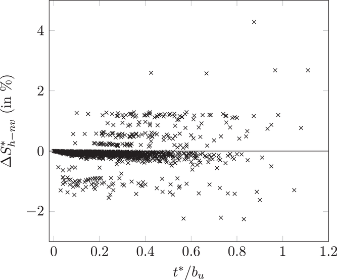
Figures 2 and 3 provide further insights into the optimal inventory policy and connect that policy to the more advanced h‐

n v

policy (

Δ Π_{h - n v}^{*}

and

Δ S_{h - n v}^{*}

measure the relative change in expected profits and expected sales, respectively, between the optimal policy and the

h - n v

policy). Figure 2 clearly shows that, not surprisingly, the benefits of the optimal inventory policy

(x^{*}, t^{*})

increase when a more delayed inventory availability is warranted (i.e., if

t^{*} / b_{u}

increases). Also, it is remarkable that the firm sometimes even finds it optimal to almost surely miss the beginning of the selling season by setting

t^{*} > b_{u}

. Conceptually, any postponement of inventory availability leads to a higher chance of the firm missing demand early in the season. Our simulation results reveal that the firm oftentimes counteracts this negative effect by (weakly) increasing its inventory quantity to promote additional sales (i.e.,

x^{*} (t^{*}) \geq x^{*} (0)

). In fact, in line with Lemma 1,

x^{*} (t^{*}) \geq x^{*} (0)

in more than 96% of our scenarios. Finally, we observe that the increase in

x^{*} (t^{*})

is largest when (a) holding costs are substantial and (b) demand is highly uncertain and likely occurs relatively late in the firm's window of sales opportunity

[0, b_{u} + L]

FIGURE 2

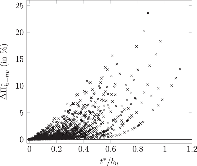
Inventory timing and firm profits

FIGURE 3

Inventory timing and expected sales

Naturally, the interaction between

t^{*}

and

x^{*}

also has an effect on the firm's expected sales; a finding that is nicely displayed in Figure 3. Even though a later inventory timing causes some early lost sales, it may also allow the firm to stock more items and thus increase overall sales (

Δ S_{h - n v}^{*} > 0

, which happens in 8.3% of our instances). In many other scenarios, the effect of a delayed inventory availability on expected sales is negligible—in only 2.6% of our scenarios, expected sales decrease by more than 1%. Hence, by coordinating its inventory timing with its inventory quantity, the firm is oftentimes able to maintain (or even increase) product sales while at the same time realizing substantial savings in inventory holding costs (on average, these savings amount to 19%).

IMPLICATIONS AND LIMITATIONS

The goals of this paper are to establish the importance of a firm's inventory timing decision and to show that inventory timing has a first‐order effect on both firm profits and customer service. We take the perspective of a firm that sells a single product over a stochastic selling season, which means that the firm has imperfect information about when exactly the selling season would be, how much demand there would be, and how demand would be distributed over the season. We motivated our analysis based on observations in the agrochemical industry; yet, similar multifaceted uncertainties are also present for other products with climatic selling seasons such as lawn and gardening items, sun care products, and nonfood specials at discount retailers. We establish the firm's optimal inventory policy, unravel the interaction effects between the firm's inventory quantity and inventory timing, demonstrate that an optimally chosen inventory timing enables the firm to increase profits and simultaneously reduce lost sales, and disentangle how the various properties of a selling season affect a firm's inventory policy. At the heart of this analysis is our insight that the firm, through its inventory timing, can endogenize (a) the profit margin of its products by determining its exposure to inventory holding costs and (b) its future demand and lost sales. We show that this flexibility may lead to a nonmonotonic interrelation between the optimal inventory quantity and timing.

A naïve approach to inventory timing might suggest to simply make products available right before the start of their selling season; yet our findings show that this thinking is flawed for two reasons. First, in many practical applications, it is not clear exactly when customer demand begins to occur (e.g., when demand depends on weather conditions). Managers thus have to determine at what moment in time their demand potential is sufficiently strong to justify inventory availability. The intuition behind this result is similar to the classic newsvendor logic that managers, when confronted with uncertain demand volumes, should not blindly maximize demand coverage. Second, even if the start of the selling season can be predicted fairly precisely, making inventory available immediately can be very costly; particularly so if inventory must be stored for a long period of time before being sold. Hence, managers—through their inventory timing—should always trade off (the risk of) losing some demand early in the season against higher profit margins for items that are sold later in the season. Our numerical analysis for a realistic range of parameters from the agrochemical industry shows that optimal inventory timing increases expected gross margins by

1 -- 2 %

, on average. While this improvement may appear relatively small, it translates into much larger improvements in net margins and absolute benefits. Moreover, our analysis also reveals that gross margins increase much more strongly, by

9 -- 10 %

, for products that face (i) strong uncertainty in demand timing or volume, (ii) a slow start of the selling season, (iii) a relatively long selling season, (iv) low‐profit margins, and/or (v) high inventory holding costs.

Like other theoretical models, ours is an abstraction of reality. In the formulation process, we chose to focus on a single‐product setting and to disregard capacity considerations. We believe that, in doing so, our framework takes a crucial first step toward the end of understanding optimal inventory timing decisions; in the real world, however, managers must coordinate the inventory timing of many different products—and especially when these products share a common (capacitated) production process. In the multiproduct case, managers must sequence the production of the different products and must therefore decide which products to produce earlier or later. That decision will directly influence each product's inventory holding costs and hence the product's effective profit margin. We view the interaction effects between different products and their inventory timing as a promising direction for future research.

Another practically relevant question concerns the specifics of the production process. On an aggregate level, we have considered production as an integrated process. Yet real‐world production processes are typically “layered”: the product passes through multiple production steps (e.g., synthesis of active ingredients, product formulation, packaging). Such a multistage production process poses additional constraints on a firm's inventory decisions. It would be instructive to explore how different production processes affect a firm's inventory timing. Last, for some practical applications, it might also be worthwhile to explicitly consider the influence of inventory availability on customer demand (see, e.g., Baron et al., 2011; Urban, 2005) and to endogenize a firm's pricing decision (see, e.g., Raz & Porteus, 2006; Petruzzi & Dada, 1999). Naturally, we would expect firms to choose an earlier inventory timing if inventory availability has a positive effect on customer demand; yet, the effect of an optimal pricing decision on a firm's inventory timing is not immediately obvious.

In sum, we believe that our work sheds light on the core trade‐offs underlying a fundamental managerial decision: a seasonal product's inventory timing. Our analysis of a firm's optimal inventory policy yields managerial recommendations as a function of the product's cost structures and the (stochastic) pattern of customer demand. Thus we have made some headway toward a better understanding of optimal inventory timing decisions for seasonal products.

Footnotes

PROOFS

ACKNOWLEDGMENTS

The authors thank the department editor, Panos Kouvelis, for his support throughout the review process. The authors are most grateful for the continuing support from the senior editor, and the thoughtful and constructive comments from two anonymous reviewers. Their suggestions considerably improved the manuscript.

ORCID

Jochen Schlapp

Danja Sonntag

References

Anupindi

Jiang

(2008). Capacity investment under postponement strategies, market competition, and demand uncertainty. Management Science, 54(11), 1876–1890.

Arrow

Harris

Marschak

(1951). Optimal inventory policy. Econometrica, 19(3), 250–272.

Axsäter

(2015). Inventory control (3rd ed.). Springer International.

Baron

Berman

Perry

(2011). Shelf space management when demand depends on the inventory level. Production and Operations Management, 20(5), 714–726.

Ben‐Tal

denHertog

De Waegenaere

Melenberg

Rennen

(2013). Robust solutions of optimization problems affected by uncertain probabilities. Management Science, 59(2), 341–357.

Böcker

Finger

(2017). A meta‐analysis on the elasticity of demand for pesticides. Journal of Agricultural Economics, 68(2), 518–533.

Bouma

(2003). GEWIS, a weather‐based decision support system for timing the application of plant protection products. EPPO Bulletin, 33(3), 483–487.

Boyaci

Özer

(2010). Information acquisition for capacity planning via pricing and advance selling: When to stop and act? Operations Research, 58(5), 1328–1349.

Cachon

Kök

(2007). Implementation of the newsvendor model with clearance pricing: How to (and how not to) estimate a salvage value. Manufacturing & Service Operations Management, 9(3), 276–290.

10.

Cachon

Swinney

(2011). The value of fast fashion: Quick response, enhanced design, and strategic consumer behavior. Management Science, 57(4), 778–795.

11.

Caseley

(1983). The effect of weather on herbicide performance. EPPO Bulletin, 13(2), 171–176.

12.

Chen

Zhang

(2009). A risk‐averse newsvendor model under the CVaR criterion. Operations Research, 57(4), 1040–1044.

13.

Choi

T.‐M.

(Ed.). (2012). Handbook of newsvendor problems: Models, extensions and applications. Springer.

14.

Comhaire

Papier

(2015). Syngenta uses a cover optimizer to determine production volumes for its European seed supply chain. Interfaces, 45(6), 501–513.

15.

Donald

(1995). A generalization of the beta distribution with applications. Journal of Econometrics, 66(1‐2), 133–152.

16.

Eeckhoudt

Gollier

Schlesinger

(1995). The risk‐averse (and prudent) newsboy. Management Science, 41(5), 786–794.

17.

Fisher

Rajaram

Raman

(2001). Optimizing inventory replenishment of retail fashion products. Manufacturing & Service Operations Management, 3(3), 230–241.

18.

Frey

Scholl

Scholz

Funke

(1973). Effect of weather on a microbial insecticide. Journal of Invertebrate Pathology, 22(1), 50–54.

19.

Gaur

Seshadri

(2005). Hedging inventory risk through market instruments. Manufacturing & Service Operations Management, 7(2), 103–120.

20.

Hadley

(1962). Generalizations of the optimal final inventory model. Management Science, 8(4), 454–457.

21.

Hadley

Whitin

(1961). An optimal final inventory model. Management Science, 7(2), 179–183.

22.

Hadley

Whitin

(1962). A family of dynamic inventory models. Management Science, 8(4), 458–469.

23.

Iyer

Bergen

(1997). Quick response in manufacturer—retailer channels. Management Science, 43(4), 559–570.

24.

Iyer

Deshpande

(2003). A postponement model for demand management. Management Science, 49(8), 983–1002.

25.

Kouvelis

Zhao

(2012). Financing the newsvendor: Supplier vs. bank, and the structure of optimal trade credit contracts. Operations Research, 60(3), 566–580.

26.

Milner

Kouvelis

(2005). Order quantity and timing flexibility in supply chains: The role of demand characteristics. Management Science, 51(6), 970–985.

27.

Nahmias

(1977). On ordering perishable inventory when both demand and lifetime are random. Management Science, 24(1), 82–90.

28.

Nahmias

(1982). Perishable inventory theory: A review. Operations Research, 30(4), 680–708.

29.

Özer

(2013). Mechanism design for capacity planning under dynamic evolution of asymmetric demand forecasts. Management Science, 59(4), 987–1007.

30.

Perakis

Roels

(2008). Regret in the newsvendor model with partial information. Operations Research, 56(1), 188–203.

31.

Petruzzi

Dada

(1999). Pricing and the newsvendor problem: A review with extensions. Operations Research, 47(2), 183–194.

32.

Petruzzi

Dada

(2010). Newsvendor models. In Cochran

Cox

Keskinocak

Kharoufeh

Smith

(Eds.), Wiley encyclopedia of operations research and management science (pp. 3528–3537). Wiley.

33.

Pierskalla

(1969). An inventory problem with obsolescence. Naval Research Logistics Quarterly, 16(2), 217–228.

34.

Porteus

(1990). Stochastic inventory theory. In Heyman

Sobel

(Eds.) Handbooks in OR & MS (Vol. 2, pp. 605–652). Elsevier, North‐Holland.

35.

Qin

Wang

Vakharia

Chen

Seref

(2011). The newsvendor problem: Review and directions for future research. European Journal of Operational Research, 213(2), 361–374.

36.

Ravindran

(1972). Management of seasonal style‐goods inventories. Operations Research, 20(2), 265–275.

37.

Raz

Porteus

(2006). A fractiles perspective to the joint price/quantity newsvendor model. Management Science, 52(11), 1764–1777.

38.

Sainz Rozas

Echeverría

Barbieri

(2004). Nitrogen balance as affected by application time and nitrogen fertilizer rate in irrigated no‐tillage maize. Agronomy Journal, 96(6), 1622–1631.

39.

Salinger

Ampudia

(2011). Simple economics of the price‐setting newsvendor problem. Management Science, 57(11), 1996–1998.

40.

Shah

(2005). Process industry supply chains: Advances and challenges. Computers & Chemical Engineering, 29(6), 1225–1235.

41.

Silver

Pyke

Thomas

(2017). Inventory and production management in supply chains (4th ed.). CRC Press.

42.

Song

J.‐S.

Van Houtum

G.‐J.

Van Mieghem

(2020). Capacity and inventory management: Review, trends, and projections. Manufacturing & Service Operations Management, 22(1), 36–46.

43.

Song

J.‐S.

Zipkin

(1996). Managing inventory with the prospect of obsolescence. Operations Research, 44(1), 215–222.

44.

Song

J.‐S.

Zipkin

(2012). Newsvendor problems with sequentially revealed demand information. Naval Research Logistics, 59(8), 601–612.

45.

Teasdale

Shirley

(1998). Influence of herbicide application timing on corn production in a hairy vetch cover crop. Journal of Production Agriculture, 11(1), 121–125.

46.

Ülkü

Toktay

Yücesan

(2005). The impact of outsourced manufacturing on timing of entry in uncertain markets. Production and Operations Management, 14(3), 301–314.

47.

Urban

(2005). Inventory models with inventory‐level‐dependent demand: A comprehensive review and unifying theory. European Journal of Operational Research, 162(3), 792–804.

48.

Van Alphen

Stoorvogel

(2002). Effects of soil variability and weather conditions on pesticide leaching—A farm‐level evaluation. Journal of Environmental Quality, 31(3), 797–805.

49.

Van Mieghem

Dada

(1999). Price versus production postponement: Capacity and competition. Management Science, 45(12), 1639–1649.

50.

Vetsch

Randall

(2004). Corn production as affected by nitrogen application timing and tillage. Agronomy Journal, 96(2), 502–509.

51.

Wang

Atasu

Kurtuluş

(2012). A multiordering newsvendor model with dynamic forecast evolution. Manufacturing & Service Operations Management, 14(3), 472–484.

52.

Wang

Tomlin

(2009). To wait or not to wait: Optimal ordering under lead time uncertainty and forecast updating. Naval Research Logistics, 56(8), 766–779.

53.

Whitin

(1955). Inventory control and price theory. Management Science, 2(1), 61–68.

Inventory timing: How to serve a stochastic season

Abstract

Keywords

INTRODUCTION

Our contributions

Related literature

MODEL SETUP

Inventory policy and stochastic selling season

The firm's optimization problem

SERVING A STOCHASTIC SEASON

The optimal inventory policy

Inventory timing and customer service

IMPACT OF CUSTOMER DEMAND PATTERN

Instantaneous demand

Deterministic selling season

QUANTIFYING THE IMPACT OF INVENTORY TIMING

Simulation setup and choice of parameters

The benchmark policies

Simulation results

IMPLICATIONS AND LIMITATIONS

Footnotes

PROOFS

ACKNOWLEDGMENTS

ORCID

References