
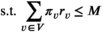
Abstract
In pursuit of Sustainable Development Goal 3 “Ensure healthy lives and promote well‐being for all at all ages,” considerable global effort is directed toward elimination of infectious diseases in general and Neglected Tropical Diseases in particular. For various such diseases, the deployment of mobile screening teams forms an important instrument to reduce prevalence toward elimination targets. There is considerable variety in planning methods for the deployment of these mobile teams in practice, but little understanding of their effectiveness. Moreover, there appears to be little understanding of the relationship between the number of mobile teams and progress toward the goals. This research considers capacity planning and deployment of mobile screening teams for one such neglected tropical disease: Human African trypanosomiasis (HAT, or sleeping sickness). We prove that the deployment problem is strongly NP‐Hard and propose three approaches to find (near) optimal screening plans. For the purpose of practical implementation in remote rural areas, we also develop four simple policies. The performance of these methods and their robustness is benchmarked for a HAT region in the Democratic Republic of Congo (DRC). Two of the four simple practical policies yield near optimal solutions, one of which also appears robust against parameter impreciseness. We also present a simple approximation of prevalence as a function of screening capacity, which appears rather accurate for the case study. While the results may serve to more effectively allocate funding and deploy mobile screening capacity, they also indicate that mobile screening may not suffice to achieve HAT elimination.
Keywords
Introduction
Goal 3 of the United Nations sustainable development goals (SDGs) is to “Ensure healthy lives and promote well‐being for all at all ages” (UN 2015). While much progress has been made in this area in recent years, “many more efforts are needed to fully eradicate a wide range of diseases” (WHO 2018b). Among the infectious diseases considered for eradication are the “big three” AIDS/HIV, tuberculosis and malaria, as well as a collection of neglected tropical diseases (NTDs). A reported 1.5 billion people required treatment for NTDs globally in 2016 (WHO 2018c). Among the NTDs are dengue, leprosy, and rabies, as well as lesser known diseases such as dracunculiasis, and human African trypanosomiasis (HAT)—also known as sleeping sickness.
In pursuit of the SDGs, the WHO has set an agenda with specific eradication and elimination targets (WHO 2018c). Eradication targets are most ambitious as they refer to reducing the global prevalence, that is, the global number of infected persons, to zero. Elimination refers to (intermediate) targets such as reducing regional or national prevalence to a given target level. For HAT, elimination is specified by the World Health Organization as a prevalence of < 1 case per 10,000 inhabitants (WHO 2018a) per focus area. This research addresses the elimination of HAT.
Given the infectious nature of HAT, timely detection and treatment form important elements of any elimination policy. Timely detection of HAT is mostly achieved through active case finding (ACF), which involves proactive screening of individuals in predetermined target groups. ACF importantly contributes to achieving the SDG related elimination goals for HAT (WHO 2013), as well as for tuberculosis (Golub et al. 2005) and leprosy (Moura et al. 2013). Remote rural areas are of special importance from the perspective of screening and treatment, as they may lack an appropriate health system infrastructure (WHO 2018a). The deployment of mobile screening teams in such areas, which actively find cases by screening the population village by village, has considerably contributed to the progress made toward elimination of HAT (Franco et al. 2017).
De Vries et al. (2016) show that the HAT prevalence dynamics vary considerably across villages and that for villages with higher prevalence levels (1 per 1000 or higher) the current WHO polices for ACF may well be insufficient to achieve the specified elimination targets. Moreover, the number of mobile teams deployed may not suffice to conduct necessary screening visits to the villages because of funding limitations. These funds tend to be diminished when prevalence decreases. Since population screening is rather expensive, this risks halting progress toward elimination, or may even result in prevalence increases (Hasker et al. 2010). Over the period 2010–2014, around 2 million people have been screened annually for HAT (Franco et al. 2017). The total yearly cost of a mobile team amounts to 130.000 USD (when using rapid diagnostic testing), resulting in a cost per screened person of 2.40 USD (Bessell et al. 2018).
Given the challenges encountered with current policies and capacities, it is important to understand the relationship between mobile screening capacity and elimination progress. Obviously, this relationship crucially depends on the planning of the mobile teams: which villages to screen and with what time intervals to screen them (cf. Mpanya et al. 2012). Yet, research on how to plan screening optimally at village level appears to be lacking (WHO 2015a). In fact, planning practices are reported to vary widely (see, e.g., Paquet et al. 1994, Ruiz et al. 2002, Simarro et al. 1990). The research question that rises is:
What are suitable methods to plan screening visits to villages by mobile screening teams and what mobile screening team capacity is required to meet prevalence level targets for HAT?
The word “suitable” requires some elaboration. On the one hand, a suitable planning method is one that leads to lowest prevalence levels. For practical purposes, on the other hand, planning methods need to be easy to understand and to implement (as is a strength of the current planning method recommended by the WHO). Hence, next to advanced exact methods, this study also proposes and analyzes simple planning policies.
Below, we review related literature, formally define the problem under consideration, model it mathematically, and prove (the optimization version) to be NP‐Hard. Moreover, using a stylized version of the model, we derive a simple approximation of the relationship between capacity and prevalence. In addition, we develop three general solution approaches and four simple planning policies. The performance of these methods and their robustness are benchmarked for a HAT region in the DRC, for which we also assess the relationship between capacity and prevalence numerically.
Literature
The treatment delay associated with both disease phases is a major enabler of sustained transmission of HAT. Patients are a potential source of infection for the Tsetse fly (Brun et al. 2010, Fevre et al. 2006) and hence indirectly for uninfected people. They may be infectious for more than 1.5 years until they start to seek care themselves, as is a form of passive case finding (PCF)) (Hasker et al. 2010). These dynamics underline the crucial importance of ACF for elimination of HAT (Hasker et al. 2010, WHO 2013). De Vries et al. (2016) study several models to capture the effects of ACF policies on HAT prevalence at village level. To be of use for village level planning, these models solely use data that are routinely collected per village: numbers of cases detected (both phases combined) and the timing of screening rounds.
The current practice of ACF is to send mobile teams to endemic villages for exhaustive population screening (Brun et al. 2010, Hasker et al. 2010, Mpanya et al. 2012). The national HAT disease control program in the DRC, for example, employs 35 such mobile screening teams. Screening campaigns are managed and coordinated on the national level (not on the health facility level). Population screening is proven to be effective (Fevre et al. 2006, Rock et al. 2015), but is also considered to be costly. The high costs are a main reason to reduce funding and thus screening activity when prevalence reduces (Hasker et al. 2010). This can in turn lead to increases in prevalence, which totaled to above 300,000 cases in 1998 alone (WHO 2015b). In 2018, the reported number of cases dropped below 1000 for the first time since the start of data‐collection 80 years ago. The DRC, our case study country, accounts for more than 80% of new HAT cases reported (Franco et al. 2017).
More recently, Deo et al. (2015) consider optimal screening, testing, and treatment for HIV/AIDS in the United States. Based on an individual disease progression model—instead of an epidemiological model—they present results on capacity requirements as well as practical policies to allocate available human resources so as to maximize health (in QALYs). Deo et al. (2013) also use an individual disease progression model to maximize deployment of scarce resources over time. The objective is to reduce the burden of disease for young patients suffering from the non‐infectious disease Asthma in the United States. They present an easy‐to‐implement, myopic heuristic that is provably optimal in special cases. These studies, as well as closely related ones, rely on a detailed multi‐stage model to capture disease progression (Bishai et al. 2007, Paltiel et al. 2005).
Various authors use extensive simulation models to study the effectiveness of HAT screening and treatment programs and the time to elimination. In addition to multiple stages of disease progression in the human population, such models typically account for vectors and animal disease reservoirs (Castaño et al. 2020, Rock et al. 2015, Rock et al. 2018). These studies typically consider one or several given screening frequencies for the population within a district. Hence, the prevalence models in these studies are homogeneous over all villages in a district (as opposed to village specific). Optimal allocation of scarcely available screening capacity, as needed to ensure screening frequencies necessary for elimination, is not considered in these studies.
In comparison to the aforementioned multi‐stage and multi‐host models, our study is less complex as it considers only one disease stage explicitly. Moreover, as data on vectors and animal reservoirs are not explicitly available at village level, our model only considers the human population. At the same time, the model presented below is more elaborate than the aforementioned models as it distinguishes the villages in which the district population lives and correspondingly relies on village specific prevalence functions. Moreover it takes travel times between villages into account, as required to model the deployment of mobile teams.
De Vries et al. (2016) present an extensive econometric analysis of HAT prevalence considering a variety of functions to model prevalence per village. The functions are validated through out‐of‐sample predictions, using data from 2004 to 2013 for 143 villages in Bandundu (DRC). This analysis identifies LMVCC, an SIS model based function in which the carrying capacity (i.e., the equilibrium prevalence level) varies per village and over time, to best fit the data. The varying carrying capacity also serves to implicitly reflect vector and reservoir dynamics per village. Although, as we elaborate below, the LMVCC model is a simplification, it solely uses data that are routinely collected on the village level, and thereby facilitates village level predictions. The optimization models and policies presented below rely on the LMVCC function to analytically model prevalence.
Literature which explicitly considers distance and travel in the deployment of scarce resources is of importance as travel time to the nearest healthcare facility is a major determinant of healthcare utilization and several types of health outcomes (De Vries et al. 2014). Providing sufficient levels of access through spatially fixed facilities is often not feasible, particularly in scarcely populated and poor areas. For this reason, mobile healthcare units are being used in several countries (see, Doerner et al. 2007, for references).
The routing problem for mobile healthcare facilities was first presented by Hodgson et al. (1998). The authors model this as a tour‐location problem, which is to select tour stops and a tour so as to minimize the total travel time and to satisfy the constraint that each demand point is covered. Hachicha et al. (2000) extend this model to the multiple vehicle case and propose three heuristics to solve it. Doerner et al. (2007) model the problem as a multi‐objective optimization problem, using coverage and travel time criteria. The main difference with this study is that we consider the health outcome measure prevalence in the objective, rather than logistic process measures such as travel time or coverage.
McCoy and Lee (2014) analyze optimal deployment of motorcycles to provide healthcare services in rural areas. The problem of determining the number of visits to each outreach site is modeled as a resource allocation problem with effectiveness and equity criteria. Effectiveness is modeled to depend (polynomially) on the number of visits. In comparison, our study is based on a HAT specific model for the relationship between visits and disease prevalence presented in De Vries et al. (2016). We refer to the PhD thesis by De Vries (2017) for generalizations of the presented models. In addition, we refer to Dasaklis et al. (2012) for an overview of scientific research on logistics operations for epidemic control.
Problem Formulation
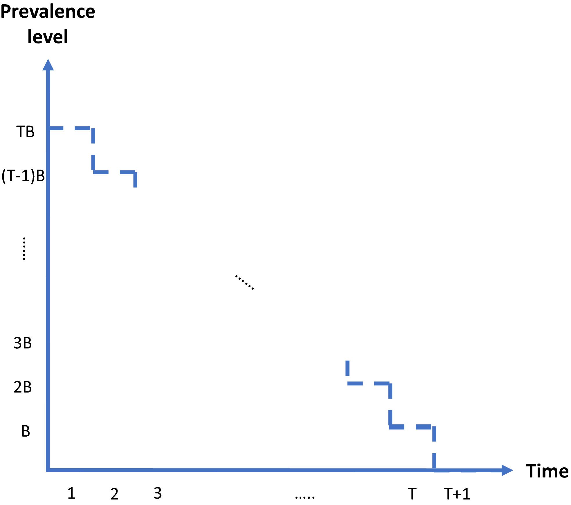
This section formally models the planning problem for mobile HAT screening teams, which we refer to as the mobile screening team deployment problem (MSTD). We consider M mobile teams, a set of villages


A planning period corresponds to one multi‐day mission, where a team visits one or multiple villages per day and camps overnight in the field to minimize travel times. In the DRC, a planning period lasts 1 month and a mission lasts 20 days (the remainder of the month is spent at home and in the office). Travel to the next village typically represents only a minor part of a screening day. Following current practice, we therefore do not explicitly model travel times but stipulate that a team stays within the same region or cluster during the planning period. A cluster


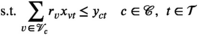
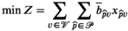
We let binary variables y
ct
indicate whether a team is assigned to cluster c in period t. For village


For each village

This assumption is justified when the exact timing of the screening round within the period has little impact on the development of the prevalence level, which is particularly the case for slowly evolving epidemics such as HAT. For ease of exposition, we henceforth always assume screening to take place at the end of the planning period.
Given the random nature of HAT infection, which depends on encounters between humans and Tsetse flies, it is not possible to exactly predict the new cases, that is, the incidence, nor the resulting prevalence. Instead, we consider expected HAT prevalence levels, as modeled in De Vries et al. (2016). We note that expected prevalence levels vary over time. As a result, they may meet elimination targets at some moments in time, but may increase to above target levels afterwards. To avoid bias toward certain time moments, the proposed model considers average expected prevalence levels. By consequence, the objective does not consider prevalence and health at the end of the planning horizon, but instead during the planning horizon.
For a given solution


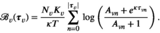
We let s
vn
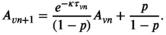
denote the stage of progression in village v after screening round n. We model a screening round to decrease the expected prevalence level with a given strictly positive impact fraction p. As elaborated in the case study (see section 6), p is the product of four variables: the average participation rate in screening rounds, the sensitivity of the screening test and the confirmation test, and the fraction of infected people who proceed to treatment (Robays et al. 2004). For example, if p = 0.8, the effect of screening in village v at stage of progression s results in reducing the prevalence level from f
v
(s) to 0.2 × f
v
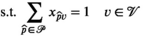
(s). Thus, screening leads to resetting the stage of progression to an “earlier” stage. The process is further explained in Figure 1 and defined by the following recursive relationship:


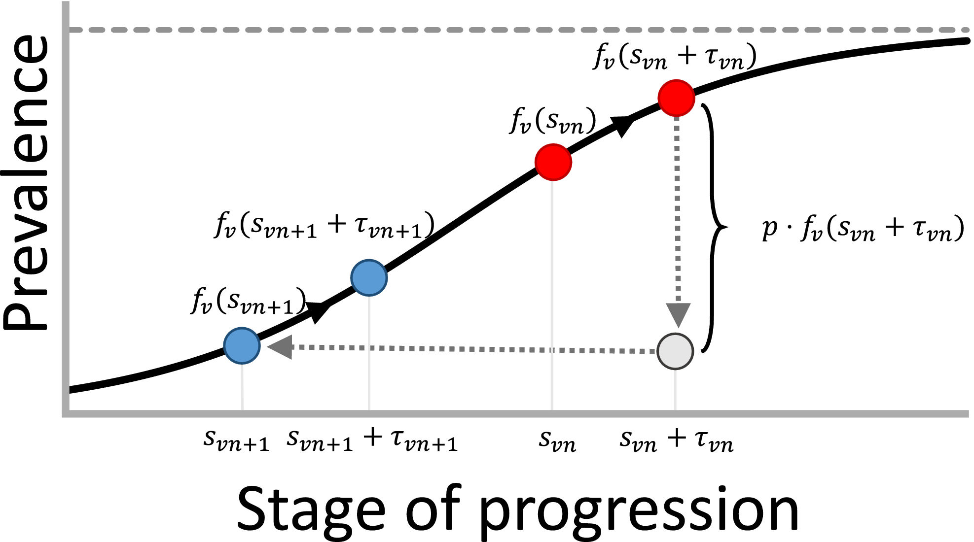
The Black Line in this Figure Represents the Prevalence Progression Function f
v
(s). After Screening Round n, We are at the Stage of Progression Corresponding to the Left Red Point, after which the Prevalence Level Develops to the Right Red Point. Next, Screening Round n + 1 Decreases the Prevalence level with Fraction p, Causing us to End up in an “Earlier” Stage of Progression: the Stage of Progression Corresponding to the Left Blue Point. Afterwards the Prevalence Level Develops to the Right Blue Point and the Process Repeats [Color figure can be viewed at
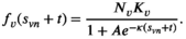
In an extensive modeling study, De Vries et al. (2016) investigate closed‐form expressions for f v (s). Based on predictive performance and theoretical justification, variants of the function corresponding to the SIS epidemic model appear most suitable. The theoretical justification lies in the observations that (1) HAT closely resembles a (multi‐host) SEIRS model (Rock et al. 2015) and (2) the number of people in the E (exposed) and R (removed) compartments are negligible given the low prevalence of the disease (De Vries et al. 2016, Rock et al. 2015). The closed‐form function for disease prevalence in an SIS model is also known as the logistic function. As illustrated in Figure 1, this function implies the expected prevalence to initially grow exponentially and to level off to an equilibrium prevalence level afterwards. This equilibrium prevalence level is called the carrying capacity and represented by the dotted horizontal line in Figure 1.
The logistic function is generic in the sense that the only information about village

According to the logistic function, after screening round n, the expected prevalence level in village v develops as follows as long as there is no screening:


We now more precisely define MSTD as problem (1)–(4) using the HAT prevalence function (8) and prove the following result by reduction from the three‐partition problem (see Appendix A):
MSTD is strongly NP‐Hard, even when

Relationship between Capacity and Prevalence
As motivated, insight into the relationship between screening capacity—that is, the number of mobile screening teams—and prevalence is crucial to assess the resource needs for reaching elimination or other targets. We provide further insight in this relationship by considering a stylized variant of the mobile screening team deployment problem (MSTD), named MSTD
R
. In MSTD
R
, the constraints that at most M teams can be deployed in each planning period t and that teams cannot visit multiple clusters in one period are relaxed. Instead, MSTD
R
requires that capacity is larger than or equal to the average capacity required per period and that each village has an infinite sequence of screening intervals of equal length, denoted by parameter τ
v
:


In Appendix A, we prove the following proposition:
An optimal solution to MSTD
R
is attained by greedily assigning screening interval
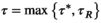
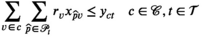
Figure 2 illustrates the implications of this finding. Our proof implies that, for village v, increasing the screening frequency


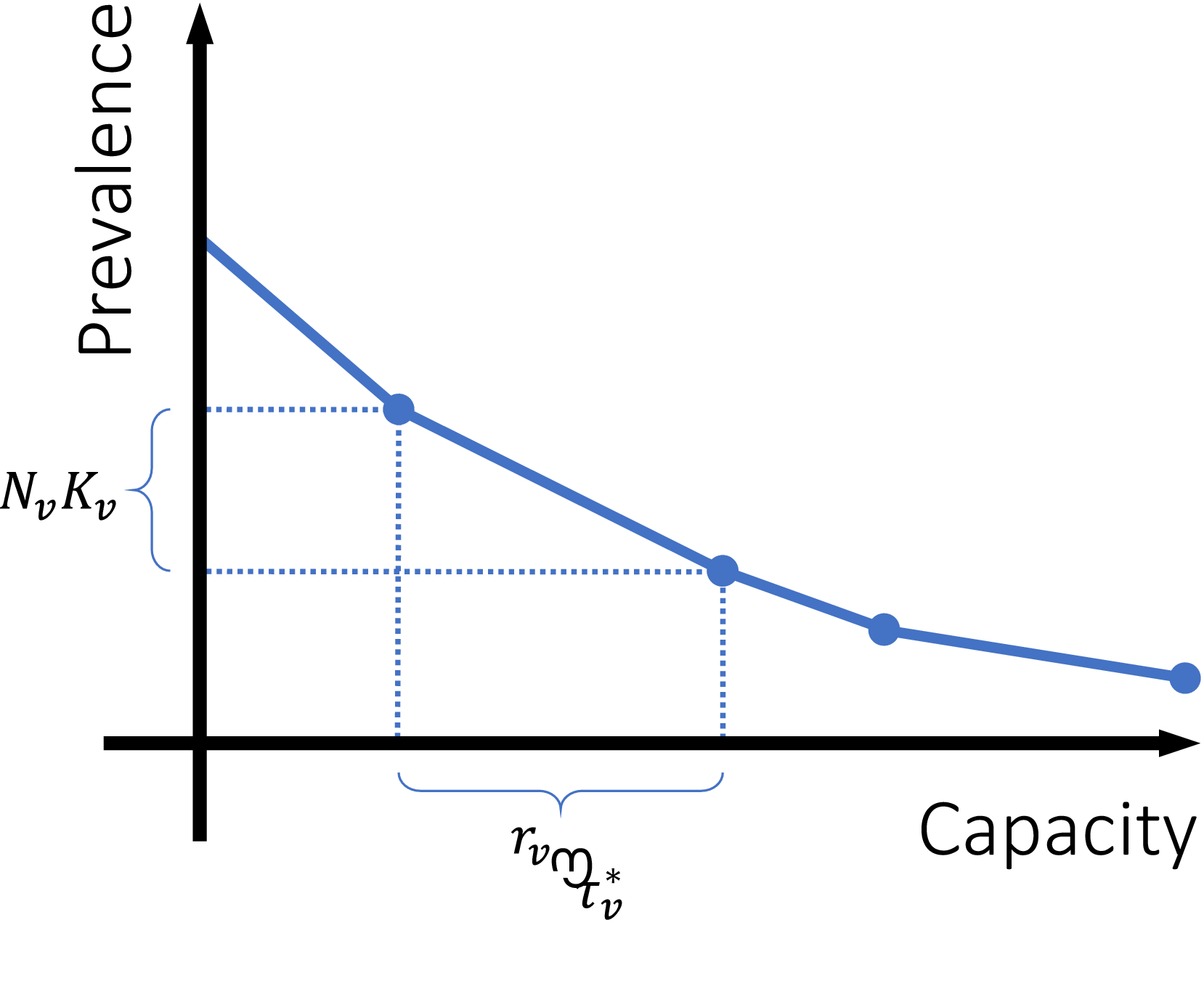
Piecewise Linear Relationship between Capacity M and Average Expected Prevalence Level [Color figure can be viewed at
Planning Methods
We present seven methods to solve problem (1)–(4). The first two methods are based on two different mathematical models which they aim to solve to (near) optimality. The third method is a heuristic, which will turn out to be especially valuable when solving larger instances. Methods four to seven are simple policies, designed for practical applicability. Below, we briefly outline each of these methods. Full details are provided in Appendix B. Although specifically developed for HAT, the methods can be applied to any disease with an increasing prevalence progression function f
v
(s) (De Vries 2017). The Binary Linear Programming (BLP) approach takes formulation (1)–(4) as a starting point and tackles the non‐linearity of The Column Generation approach uses a mixed‐integer programming (MIP) formulation that defines MSTD in terms of visit schedules or visit patterns. The problem then boils down to selecting a visit pattern for each village and allocate teams to clusters. Constraints are that each village can only be visited in periods in which a team is assigned to its cluster and that in each period no more than M teams are assigned. This problem has exponentially many variables, but can be approached through column generation. The column generation subproblem that emerges can be solved as a shortest path problem, using discretization techniques (as used to solve the BLP formulation), which are further elaborated in Appendix B.2 (along with other algorithmic details). The method generates columns until the LP relaxation is solved to optimality, and then solves the binary version with the set of generated columns. Hence, this approach is not necessarily optimal.
Iterated Local Optimization iteratively improves the current solution (
The Equalization Policy equalizes screening frequencies of the villages. We define The Differentiation Policy generalizes the Equalization Policy. It first classifies villages into several classes ec (e.g., high and low), depending on past prevalence. In addition, it assigns to each class ec a target screening interval τ
ec
. Next, in period t, we first determine for each cluster c the number N(t, c) of people for which the time since the last screening equals at least their target interval. Assignment of teams to clusters and to villages within the clusters is done as in the Equalization Policy. The present WHO policy is a Differentiation Policy. The Max Cases Policy strives to maximize the number of cases detected per planning period. For each cluster c, it calculates l
1(c), the total expected prevalence at the beginning of the period among villages screened in that cluster if a team would be assigned to it. Within a cluster, villages are selected for screening in decreasing order of the ratio of expected number of cases among the people screened in village v over r
v
. This can be interpreted as the expected number of cases detected per time unit spent screening in village v. Next, the policy assigns teams to the M clusters with highest l
1(c). The Prevalence Increase Policy strives to screen villages for which no screening would lead to a relatively large increase in expected prevalence. For each cluster c, it calculates l
2(c), the total expected increase in prevalence averted for the villages screened in that cluster if a team would be assigned to it. Within a cluster, villages are selected for screening in order of highest prevalence increase per time unit spent screening. Next, the policy assigns teams to the M clusters with highest l
2(c).


Case Study
This section addresses our research question for a case study on HAT screening in the Kwamouth health zone in the Bandundu province of the Democratic Republic of Congo. The DRC accounts for 80% of new HAT cases reported (Franco et al. 2017). We first analyze the methods designed to find (near) optimal solutions, to assess their computation times and solution values. We subsequently use one of these methods as a benchmark for the performance of the practice oriented policies in terms of average expected prevalence reduction. Next, we analyze the validity of our insights on the relationship between prevalence and capacity (see section 4). To provide insight into the robustness of the results, we also present sensitivity analyses with respect to data impreciseness. Additional results on end of horizon effects and determinants of optimal solutions can be found in De Vries (2017). The methods were implemented using Matlab R2015a and used CPLEX 12.63 as a BLP solver.
Baseline Case Description
The case study contains 239 villages in the Kwamouth health zone, and is derived from HAT screening data from 2324 villages between 2004 and 2013 (see De Vries et al. 2016, for the data). The 239 villages were included when there exists at least one record of the number of people screened and the geocoordinates of the village are known. The first criterion is required to estimate population sizes and the second is required for assigning villages to clusters. We excluded 463 villages (at least partly) due to lacking geocoordinates. In 114 of the excluded villages, HAT cases were found in at least one screening round. The average number of cases per visit to these villages was 1.90.
The average participation rate per screening round, which we denote by part, has been reported to be 71% (of the population) and to vary substantially in Bandundu (Robays et al. 2004). Hence, for now we estimate the total village population to be 1.2 times the maximum number of people participating in a screening round reported for that village, and revisit participation in the sensitivity analysis. To ensure that each village can be screened in one planning period, one large village had to be split into two halves. Both are considered separate villages in the remainder of our analyses, which increases the total number of villages to 240.
Current planning practices in the national sleeping sickness control program of the DRC largely support cluster‐based planning, by which teams select a cluster per planning period of 1 month, in which they only visit villages in the selected cluster (E. Hasker, personal communication, 20‐9‐2016): “They define different axes, and then simply visit one axis per trip. (...) An axis can be a major road or a river by which you travel. Of course, there are not many roads. Most villages can only be accessed by one road, so if you are traveling in a given direction, it is logical to stay in that region.”
“The planning assumes that they screen 300 persons per day, 20 days per month, so 6000 [persons] per month, and then they return to their bases.”
We manually clustered the villages, following the structure of the road network. The resulting clusters, the villages, and their relative population sizes are depicted in Figure 3.
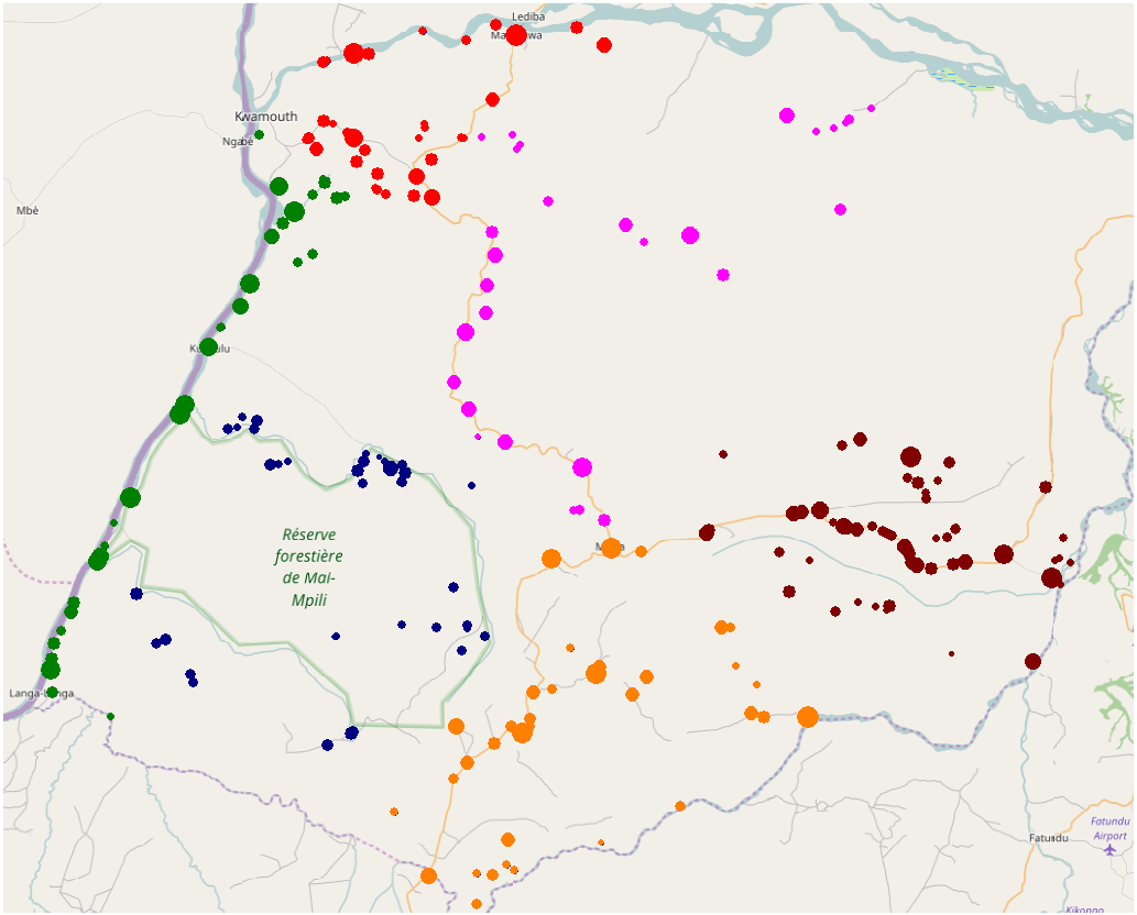
Map of the 240 Villages in Kwamouth Included in Our Case Study. Clustering is Indicated by Color. Population is Indicated by Node Size [Color figure can be viewed at
Reflecting current practice in the DRC, we assume that a team can screen 6000 persons per planning period. As the number of people participating in a screening round in village v equals part·N v , we estimate that screening of village v takes r v = part·N v /6000 of a planning period (where part was defined as the average participation rate). Since the total estimated number of people from the 240 villages participating in screening equals 73,521, one team would need approximately 12 months to visit the villages, which is in line with the current WHO guidelines for villages having one case in the past 3 years (WHO 2015a).
For 70 villages we were able to obtain the carrying capacities as percentages of the population from De Vries et al. (2016). Since sufficient screening data were lacking for the other villages (required are at least two screening rounds and at least one disease case) these were randomly generated from an exponential distribution with mean 0.858%. This distribution was based on 143 carrying capacities estimated for this region by De Vries et al. (2016). We do not claim these estimates to be accurate, but consider them to be realistic enough for the purpose of the computational analysis presented in this case study. We also note that it is realistic to assume that required data will be available on a large scale in the future: the national HAT control program in the DRC recently started digital data collection (Bluesquare 2018, Hasker et al. 2018).
Baseline values for the impact related parameters introduced in section 3 as well as other parameters used in the case study can be found in Table 1. We denote the sensitivity of the screening test and the confirmation test by sens scr and sens con , respectively. Parameter treat represents the fraction of infected people who proceed to treatment. We note that time is measured in months. We consider a planning horizon of 36 months to examine how the practice oriented policies—which look at the past (Equalization and Differentiation), the current situation (Max Cases), or 1 month ahead (Prevalence Increase)—perform in the long term.
Baseline Case Parameters
(Near) Optimal Methods
To identify which of the first three solution methods proposed in section 5 could serve as a suitable benchmark for the practice oriented policies, we now consider their computation times and solution quality. To allow the calculation of the exact solution and hence of exact optimality gaps, we first consider small instances in which T ranges from 4 to 7 months, and M ranges from one to two mobile teams. The binary linear programming (BLP) approach uses a discretization consisting of 25 prevalence levels equally spaced between zero and the villages’ carrying capacities. The exact solution was determined by applying this approach for a discretization containing all 2 T prevalence levels attainable. Table 2 shows the CPU times (sec.) and optimality gaps for the three methods.
Computational Results
Each of the methods yields optimal solutions or solutions within 0.1 % of optimality for all instances. Yet, computation times for the BLP approach soon become impractical for a discretization using 25 prevalence levels. For the other approaches, solution times grow much more slowly, which renders them more suitable for large problem instances, such as instances considering up to 36 months, as in the case study at hand.
To assess the added value of the column generation approach over the iterated local optimization (ILO) approach, we also applied these two methods to T ∈ {12, 18, 24, 30, 36}. In each case, the approaches attain the same solution value. As the ILO is much faster, we use the solutions it produces as a reference in the remainder of this case study and refer to them as “optimized” (rather than “optimal”) solutions.
Performance of Practice Oriented Policies
Figure 4 compares the prevalence levels resulting from applying the policies introduced in section 5. Here, the Differentiation Policy divides villages into four equally sized classes. The first class contains the villages with highest K v , etc. The policy assigns the classes 40%, 30%, 20%, and 10% of the screening capacity, respectively.
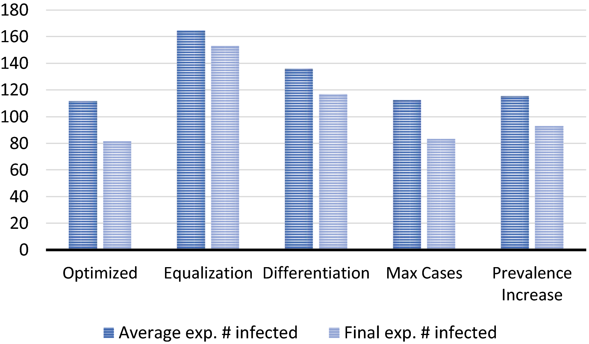
Average and Final (end of planning horizon of 36 months) Expected Number of People Infected in the 240 Villages for the Optimized Schedule and the Schedules Following from the Planning Policies [Color figure can be viewed at
Without screening, the average expected number of people infected in the 240 villages during the next 36 months would be 341 persons. Hence, the solutions avert 52% (Equalization) up to 67% (Optimized) of average expected prevalence, which shows the substantial impact active case finding can have. Surprisingly, despite their simplicity, the Max Cases and Prevalence Increase Policies perform only 0.7% and 3.4% worse than optimized planning, respectively. The slightly poorer performance of the second might well be caused by the s shape of the prevalence progression function, which implies that prevalence growth is steepest for modest prevalence values, thus foregoing villages with higher prevalence (yet lower prevalence increase). The Equalization and Differentiation Policies perform substantially worse.
To better understand these results, let us zoom in on the planning decisions recommended by the different methods. Figure 5a describes how the different methods “allocate” screening capacity over the population. We order the population along the x‐axis in decreasing order of carrying capacity of the villages in which they live and depict on the y‐axis the allocated percentage of screening capacity (in terms of people screened). A straight line from the origin would mean a perfectly equal distribution. The (near‐) horizontal parts of the curve for Prevalence Increase support the hypothesis that it neglects several villages where prevalence is high but not strongly increasing. The curves for Optimized screening and the Max Cases policy are rather similar. The main difference is that Max Cases screens slightly more people overall.
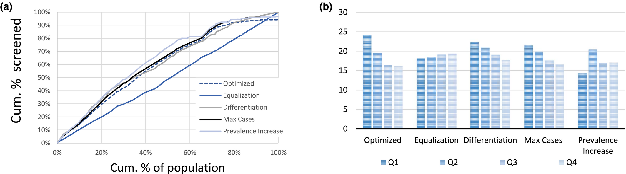
Baseline Case Solution Characteristics (a) Distribution of the Number of Visits Over the Population. Individuals are Ordered along the x‐axis in Decreasing Order of their Carrying Capacity and (b) Average Visit Period for People in Villages with Carrying Capacities in the Lowest (Q1), Second Lowest (Q2),… Quartile of the Carrying Capacity Distribution [Color figure can be viewed at
To understand why optimized screening outperforms Max Cases, we must zoom in on the timing of the screening rounds, which is analyzed in Figure 5b. Here, we depict the “average visit period” for people living in villages with a carrying capacity that is in the lowest quartile (Q1), the second quartile (Q2),…1 For example, visits in period 10 and 20 yield 15 as the “average visit period.” The figure shows that optimized planning visits villages with a high carrying capacity relatively early: in comparison with Max Cases, the average visit period is 0.6 days earlier for villages in the highest quartile and 1.1 days earlier for villages in the second highest quartile. It thereby preventatively controls the epidemic in these villages. Max Cases, instead, is more reactive as it solely screens a village when the expected prevalence is relatively high. This insight will explain some of the observations presented below.
To assess the sensitivity of our results to changes in characteristics of our case study, we analyzed three additional variants. The first considers the situation when cases are concentrated in fewer villages. The second uses population numbers from the WorldPop database, which are estimated on the basis of satellite images (see Tatem et al. 2007). The third clusters the villages randomly. Results are described in Appendix C and confirm our findings: (1) solutions obtained for these cases avert 51%–68% of average expected prevalence, (2) the Max Cases and Prevalence Increase Policies perform only 0.8%–1.3% and 1.6%–3.0% worse than optimized planning, and (3) the other policies perform substantially worse. Numerical results presented in Appendix C suggest that our conclusions are also rather robust to excluding villages.
Accuracy of Capacity Estimation Method
Figure 6 depicts the accuracy of the capacity estimation method derived in section 4. The solid line represents the piecewise linear relationship between capacity and average expected prevalence estimated by this method. The dashed line represents the actual average prevalence level over the next 30 years when the number of people who can be screened per planning period equals 0, 100, 200, …, 10,000, as attained by the optimized solution. (As explained, one could alternatively express capacity scenarios in terms of the number of mobile teams. However, as our case study is relatively small, this would yield few data points.)
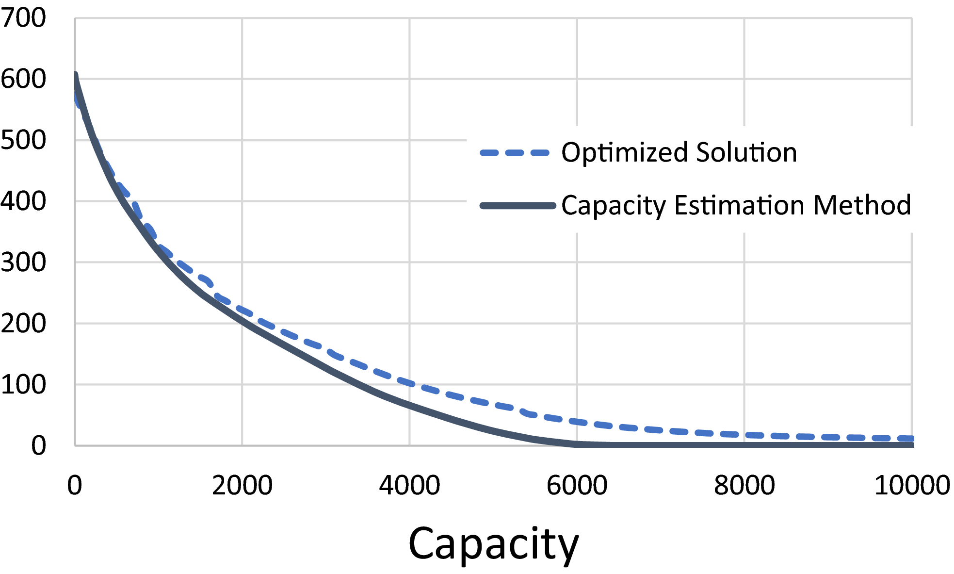
Average Expected Prevalence Level vs. Capacity (# people screened per planning period). Dashed line: Average Prevalence Level Over the Next 30 Years Corresponding to the Optimized Solution. Solid line: Average Prevalence Level Over an Infinite Horizon, as Estimated by the Method Derived in Section 4 [Color figure can be viewed at
Despite neglecting routing considerations and the finite planning horizon, the capacity estimation method provides a rather accurate estimation of the capacity needed to reach a given prevalence level target. The average vertical difference between the curves equals 25 people (maximum difference: 45). The average horizontal difference (for the parts of the graph where it can be calculated) equals 330 persons or 5.5% of a team's capacity. We note that the method's accuracy appears relatively high for high prevalence levels and vice versa for lower ones. For the part of the curve where capacity ≤ 3000, the difference is 8% (measured as a percentage of the optimized solution value). For the part where 3000 < capacity ≤ 6000, this average difference is 54%, while for 6000 > capacity, the average difference is 100%. This could be explained from the slow convergence toward eradication during the 30 years, which the method neglects by analyzing average prevalence over an infinite planning horizon. Next to model accuracy, which we shall discuss later, this provides a second argument to primarily use this result in the context of relatively high prevalence levels.
Although we leave formally proving this to future research, we hypothesize that the method provides a lower bound on the actual capacity required in case of an infinite planning horizon. (Note: our stylized model not only relaxes capacity constraints but also restricts solutions to constant screening intervals.) Our results suggest that the method generally provides lower bounds in case of a finite horizon as well.
Sensitivity Analysis: Carrying Capacities
As we cannot directly observe the carrying capacities of the villages, we estimate them from observables. De Vries et al. (2016) propose and fit a formula relating the carrying capacity to the average observed prevalence and the average screening frequency in the past 5 years. Due to stochasticity in prevalence levels, however, such estimates may be imprecise, which begs the question to what extent this impacts the quality of scheduling decisions. Figure 7 summarizes sensitivity analysis results. For each village, we randomly draw the “real” value of K v according to a uniform distribution on [K v (1 − Δ), K v (1 + Δ)], determine the “real” optimized solution, and calculate the “real” value of the solutions that were based on the “incorrect” carrying capacities. This is repeated 100 times for each Δ ∈ {0.2, 0.4, 0.6, 0.8, 1.0} which yields the depicted average and maximum observed optimality gaps.
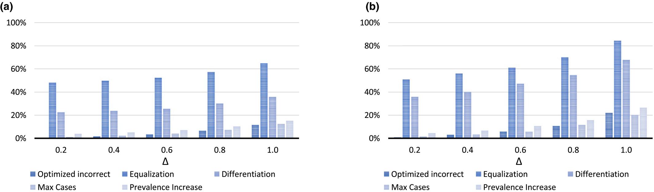
Results of the Sensitivity Analysis on Carrying Capacity Estimates (a) Average Optimality Gap (%) based on 100 Draws and (b) Maximum Optimality Gap (%) in 100 Draws [Color figure can be viewed at
The results show that solution quality is rather robust with respect to impreciseness. For example, the estimated “optimality” gap for the Max Cases Policy ranges from 1.0% for Δ = 0.2 to 12.3% for Δ = 1.0. Hence, even when the real carrying capacities deviate up to 100% from the assumed values, the estimated average gap for this policy equals only 12.3%. Furthermore, the maximum observed “optimality” gap is rather close to the average. For the solution obtained by the Max Cases Policy, for example, the maximum ranges from 1.5% for Δ = 0.2 to 20.3% for Δ = 1.0. Note that the actual optimality gap may be larger since we used the optimized solution for comparison.
Sensitivity Analysis: Screening Impact
There is an ongoing debate about the expected impact of active case finding (Welburn et al. 2016), which is known to vary among regions (Robays et al. 2004) and may change over time. As a consequence, the true impact of screening may deviate from the assumed impact, as quantified by parameter p. Figure 8 depicts how the quality of solutions obtained for baseline value p = 0.5 (which follows from the values in Table 1) is affected when p equals 0.1, 0.3, 0.7, or 0.9 in reality. Here, “optimized incorrect” refers to the optimized solution using p = 0.5. We use the optimized solution for the “real” values of p to estimate optimality gaps.
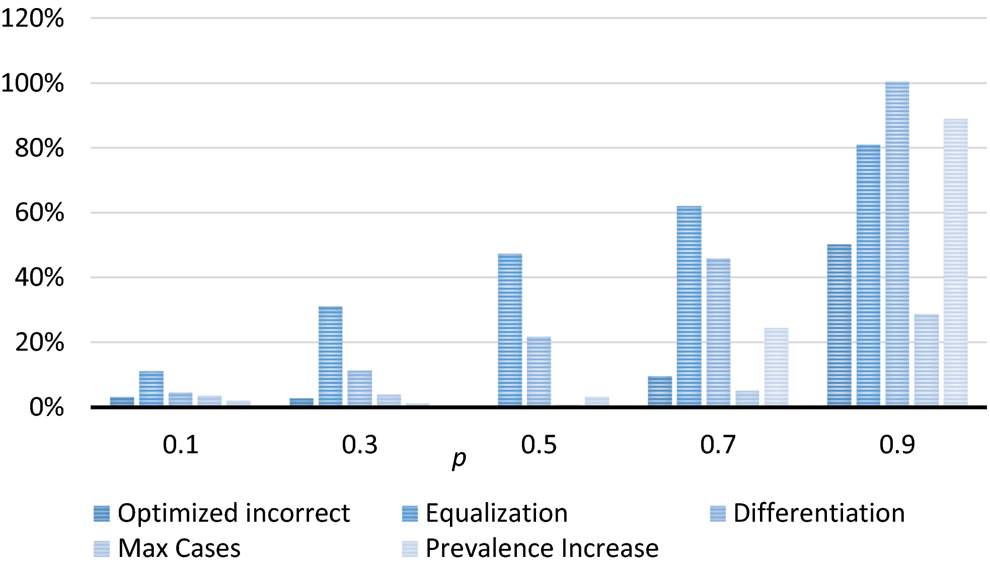
Optimality Gap Attained when Basing Decisions on the Baseline Value for p, for Different Actual Values of p [Color figure can be viewed at
We observe that the estimated optimality gap for the optimized schedule using p = 0.5 is only 3.1%, 2.7%, and 9.4% when in reality p equals 0.1, 0.3, and 0.7, respectively. This shows that even a substantial over‐ or underestimation of impact does not necessarily have serious consequences. When p equals 0.9 in reality, however, sub‐optimality increases to 50.2%. An explanation is that, as explained in section 6.3, optimized planning has the incentive to screen villages with low expected prevalence levels but high carrying capacities, so as to control the epidemic and prevent high prevalence levels. Such solutions, however, tend to overly focus on such villages in early planning periods when p is larger than the assumed value and thereby miss opportunities to address the epidemic in other villages.
The Max Cases Policy is more resistant to this because it focuses efforts on areas where expected prevalence is highest. As a consequence, it outperforms optimized planning by 4.5 and 21.4 percent points when p equals 0.7 and 0.9 in reality, respectively. This strengthens the belief that this policy provides a good alternative to optimized planning. The Prevalence Increase Policy overly focuses on preventing prevalence from increasing, rather than maximizing prevalence decrease. The lack of focus on the latter becomes particularly visible when the screening impact is high. For example, the gap with optimized planning equals 38.7 percent points when p equals 0.9 in reality. The schedules obtained by the Equalization and Differentiation Policies remain inferior to the optimized schedules, irrespective of p.
Sensitivity Analysis: Stochastic Participation
Our model implicitly assumes that the participation level in a screening round is fixed. In reality, however, participation is stochastic. This section examines how the quality of planning decisions is affected when participation in screening round n in village v, part vn is uniformly distributed on [part(1 − Δ), part(1 + Δ)], with Δ ∈ {0.05, 0.10, 0.15, 0.20, 0.25}. We randomly generate part vn for our baseline case, determine the “real” optimized solution (i.e., the optimal solution value when participation is known in advance) and determine the “real” value of solutions that were based on the assumption that part vn = part. This process is repeated 100 times for each value of Δ. Figures 9a and b depict the average and maximum observed optimality gaps.
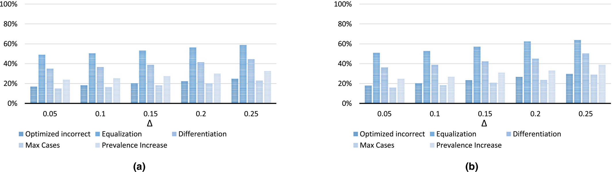
Results of the Sensitivity Analysis on Carrying Capacity Estimates (a) Average Optimality Gap (%) based on 100 Draws and (b) Maximum Optimality Gap (%) in 100 draws [Color figure can be viewed at
The results again show that the Max Cases Policy outperforms the other practice oriented policies and optimized planning. The latter could again be explained from the insight presented in section 6.3: optimized planning has the incentive to screen villages with low expected prevalence levels but high carrying capacities. This is, however, too conservative in expectation. For example, if participation is high for just one screening round, this can substantially reduce screening efforts needed afterwards (cf. De Vries et al. 2016).
Conclusions and Discussion
In pursuit of Sustainable Development Goal 3, considerable global effort is directed toward elimination and eradication of infectious diseases in general and Neglected Tropical Diseases in particular. For various such diseases, the deployment of mobile screening teams forms an important instrument to reduce prevalence toward the disease elimination goals. There is considerable variety in planning methods for the deployment of these mobile teams in practice, but little understanding of their effectiveness. Moreover, there appears to be no systematic understanding of the relationship between capacity, for example, in number of teams, and progress toward the goals.
We have addressed these research topics for the neglected tropical disease HAT and establish that the planning problem is strongly NP‐Hard. Moreover, we presented exact solutions methods and a relatively simple approximation of the relationship between capacity and prevalence. We empirically analyze the methods for a case study on a HAT region the Democratic Republic of Congo, and present two practically feasible planning policies which yield near optimal solutions. Moreover, the presented approximation of prevalence as a function of capacity appears rather accurate for the case study.
To assess the quality of solution methods we firstly developed and tested two (near) exact methods and an iterative heuristic. For the case study at hand, the heuristic delivers solutions which are very close to optimal (within 0.1%), referred to as optimized solutions. Moreover, it is fast enough to provide optimized solutions for the larger case study instances.
For the purpose of practical implementation in remote rural areas, we developed simple, practical policies, and bench marked their performance against the optimized solutions. The Equalization Policy—which strives to visit all villages equally often—performed poorest. It was outperformed by a generalization of this policy, the Differentiation Policy, which partitions the set of villages into classes, and subsequently strives to equalize visits per class. The Differentiation Policy shares some commonalities with the current WHO policy which distinguishes three classes. The prevalence resulting from the Differentiation Policy is still substantially above optimized prevalences.
The Max Cases Policy prioritizes in each planning period villages which have highest prevalence at the beginning of the planning period, per unit of time required to screen the village. The Prevalence Increase Policy prioritizes the villages with largest growth in prevalence if left unscreened, per unit of time required to screen the village. Despite their simplicity, the Max Cases and Prevalence Increase Policies yield decisions that are only 0.7% and 3.4% worse than optimized decisions in the baseline case. The near optimality of these policies and the slightly better performance of the Max Cases policy remain valid for three variants of the baseline case. As implementation of Max Cases policy only requires monthly (access to) current prevalence estimates, it appears intuitive and feasible to implement. Given its near optimality, we strongly recommend conducting an experimental study to implement and empirically evaluate the Max Cases policy.
The sensitivity analyses suggest that solution quality is relatively insensitive to inaccuracy of input data for the better performing solution methods. This is important because of the difficulty to collect accurate data in relevant settings. Larger inaccuracies, however, likely result in substantial sub‐optimality of solutions. Thus we stress that the investment in mobile screening teams is considerable more effective when accompanied by investments in data collection for reliable parameter setting. We note that particularly the Max Cases policy appears robust to inaccuracies, which strengthens the belief that this policy provides a good alternative to optimized planning.
For the case study, our computational results show that the presented approximation of prevalence as function of capacity forms a practical proxy. The insight it can provide into the capacity required to achieve and maintain a prevalence level—which has been repeatedly problematic in the past—is particularly valuable. The capacity estimates enable to set or update capacity cost‐effectively, instead of relying on experimental budget reductions which undo previously achieved prevalence reductions.
Our results indicate very substantial reductions in prevalence levels from mobile screening for the population of 73,512 people considered. More specifically, they estimate prevalence without screening to increase to 494 over a period of 3 years, whereas optimized screening can bring it down to 81 and the Max Cases Policy to 83. This confirms the empirical finding that the effectiveness of mobile teams greatly contributes toward elimination (Franco et al. 2017). At the same time, even optimal screening for 3 years still results in a prevalence level exceeding 1 case per 1000, more than 10‐fold the goal set by the WHO (which implies a total prevalence target of seven or lower for the case at hand). Despite the effectiveness, we therefore doubt whether mobile screening team deployment will lead to the elimination goals in the case study region, especially so as it will remain tempting to cut the large screening expenses when prevalences become low. Our results may be viewed to confirm that alternative, innovative, approaches may be required to achieve the WHO targets. Current developments to improve the accessibility of treatment, for instance through the oral medication Fexinidazole may lead to this direction.
One may doubt whether the presented functions for expected prevalence remain accurate when prevalence levels approach zero, and hence whether the presented models continue to give reliable insights. To better understand how to achieve the ambitious elimination goals of the WHO, we therefore call for the development of (discrete event simulation) models which simulate cases explicitly, rather than relying on continuous expected prevalence. Such models also allow to analyze policies which update prevalence functions and allocation decisions dynamically, based on cases found. The cases found can then additionally include cased found by passive case finding, which have been disregarded in our study.
Future modeling work could also examine innovative case finding approaches. There have been promising pilot studies involving mini, motorcycle‐based, teams (Snijders et al. 2020) and a targeted door‐to‐door (TDD) approach (Koffi et al. 2016). The expected impact of a screening round on prevalence likely differs in comparison to traditional teams, due to differences in participation and diagnostic algorithms. This raises novel questions regarding the optimal case finding approach depending on context, how optimal screening frequencies differ per approach, and how different types of teams can complement each other (cf. Snijders et al. 2020).
Finally, future research could investigate more elaborate models or approximations of prevalence progression. Examples include models that incorporate multiple disease hosts (Castaño et al. 2020, Rock et al. 2015, 2018) and models that explicitly distinguish multiple disease stages, for example, the exposed, asymptomatic, and symptomatic phases (cf. Deo et al. 2013, 2015). An interesting resulting question then arises regarding the cost effectiveness of additional data collection: are the resulting gains towards elimination worth the additional costs of implementation and village level data collection? (cf. De Vries and Van Wassenhove 2020).
The WHO has not only formulated elimination goals for HAT, but also for other infectious diseases. For several of these diseases, among which is tuberculosis, screening by mobile teams is an important instrument in the efforts toward elimination. The methods we propose, and in particular the practical policies that perform very well, are general enough to be applied to other diseases. Of course, such application requires the present HAT specific average expected prevalence function to be replaced by another function, specific to the disease under consideration. It will be of interest to learn whether the Max Cases Policy and Prevalence Increase Policy again perform so well, and hence are more broadly of value to effectively reach elimination goals. Further research in this direction is encouraged.
Proofs
Consider a three‐partition instance with target value B and positive integers B/4 < r
i
< B/2 for i ∈ {1, … , 3T} and a target value B such that A polynomial‐time reduction from three‐partition to MSTD is obtained as follows. We consider T + 1 planning periods, one cluster of villages, and one screening team. For each integer i ∈ {1, … , 3T}, we introduce a village v(i), resulting in 3T villages. For i ∈ {1, … , 3T}, village v(i) requires screening capacity r
v(i) = r
i
/B. Moreover, village v(i) has parameter values N
v(i) = r
i
, K
v(i) = 1, and A
v(i)0 = 0. There is one team available. We set We now claim that the three‐partition instance I is a yes‐instance if and only if the MSTD instance has a solution of value at most
The prevalence level at the beginning of the planning horizon equals
Note that the decision version of MSTD is in NP since we can calculate the value of a solution in at most 


Prevalence Level Over Time in the MSTD Instance if the 3‐Partition Instance is a yes‐Instance [Color figure can be viewed at
Let 
Screening village v with constant interval τ
v
yields average prevalence level: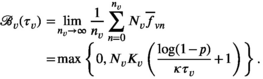
Our summation is the Cesaro mean of the sequence 
The following lemma implies that we can get rid of the maximum operator in Equation (A1):
There exists an optimal solution to Problems (10)–(12) in which the screening interval is at least 
Suppose there exists an optimal solution with τ
v
< τ*. Then increasing τ
v
to τ* does not change the value of function (A1) and does not violate capacity constraint (11). The fact that τ* > 0 follows from the assumption that p > 0.
Enforcing this lower bound implies that the second term in Equation (A1) is nonnegative. Based on this observation, Problems (10)–(12) can be formulated as the following LP problem: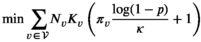
Here, 


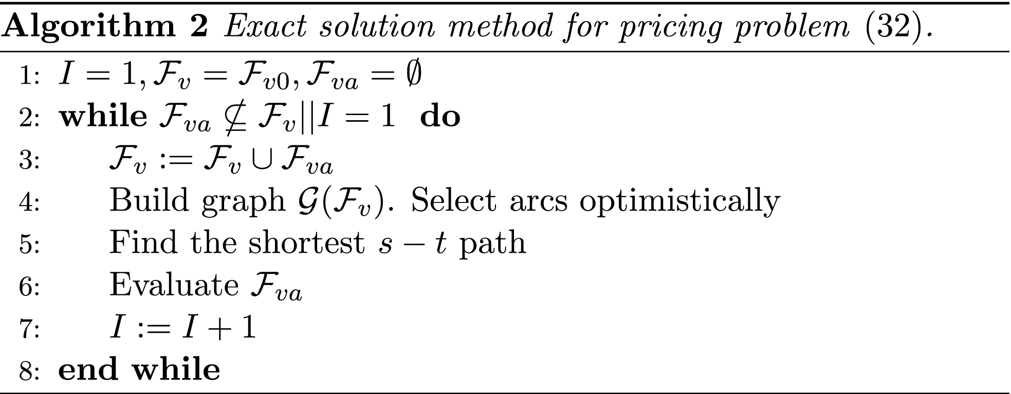
Details on Planning Method
BLP Approach
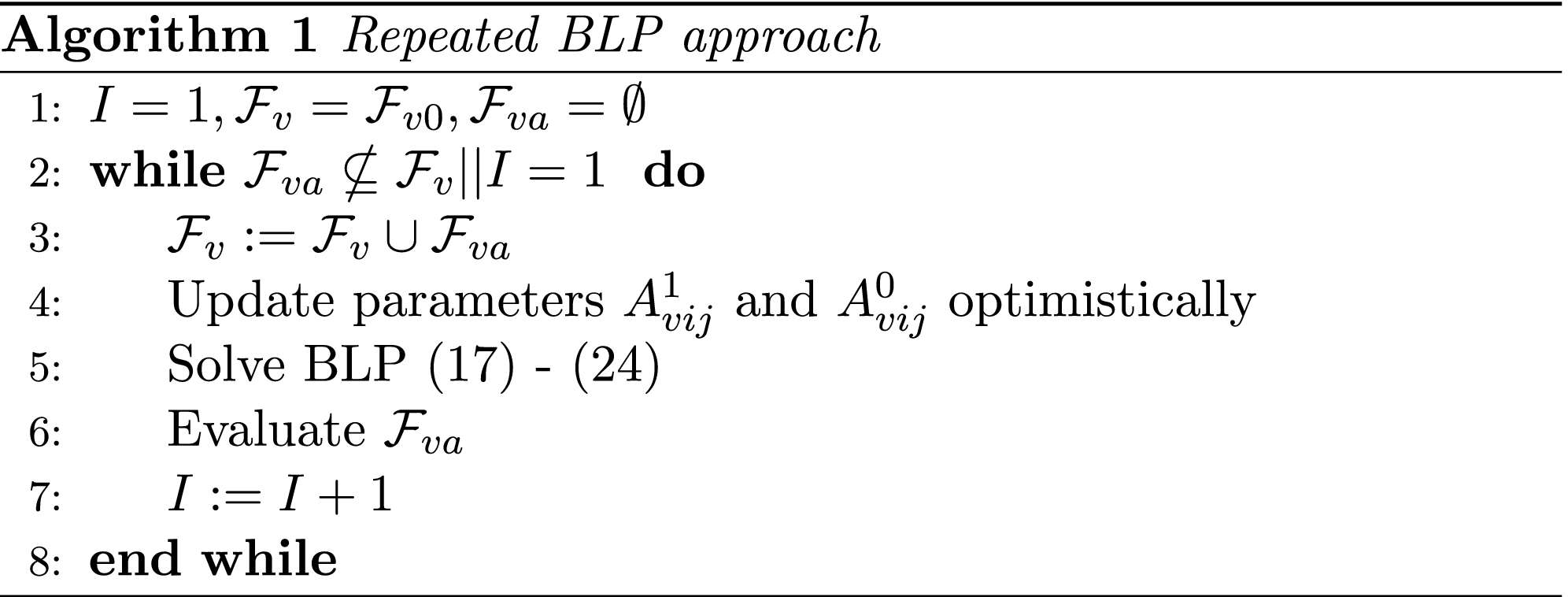
The binary linear programming (BLP) approach takes formulation (1)–(4) as a starting point and tackles the non‐linearity of function 
Let 


Since we assume each screening round takes place at the end of a planning period (see section 3), the average expected prevalence level during period t only depends on the prevalence level i at the beginning of that period. Let parameters 

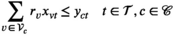
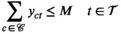

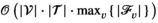
The proposed discretization may restrict the optimization to an incomplete set of relevant prevalence levels and hence may imply incorrect solution values and sub‐optimal solutions. Discretized formulations can, however, be ensured to be exact in the following two ways. First, we can pre‐calculate all attainable prevalence levels and include them into 
As an alternative, we can repeatedly solve the model while adding the actual set of prevalence levels 


Column Generation Approach
An alternative approach is to formulate the problem in terms of selecting a visit schedule or visit pattern for each of the villages. Let 


As is standard practice, our column generation approach starts from solving the so‐called master problem (MP)—the LP relaxation of problems (B9)–(B13)—using only a subset of the visit patterns. The resulting problem is referred to as the restricted master problem (RMP). Next, “promising” patterns are identified in the so‐called pricing problem, and added to the RMP. This process is repeated until no more promising patterns can be found. The resulting set of patterns is then added to Equations (B9)–(B13), which can subsequently be solved to optimality using integer programming techniques. Notice that this approach is not necessarily exact, as the optimal solution to Equations (B9)–(B13) may require patterns which have not been included or generated to find the optimal solution to the LP relaxation.

In solving the pricing problem, we again encounter the difficulties caused by the non‐linearity of the prevalence progression function. We deal with this as follows. First, we again discretize the progression function f
v
(s), yielding the set of prevalence levels 


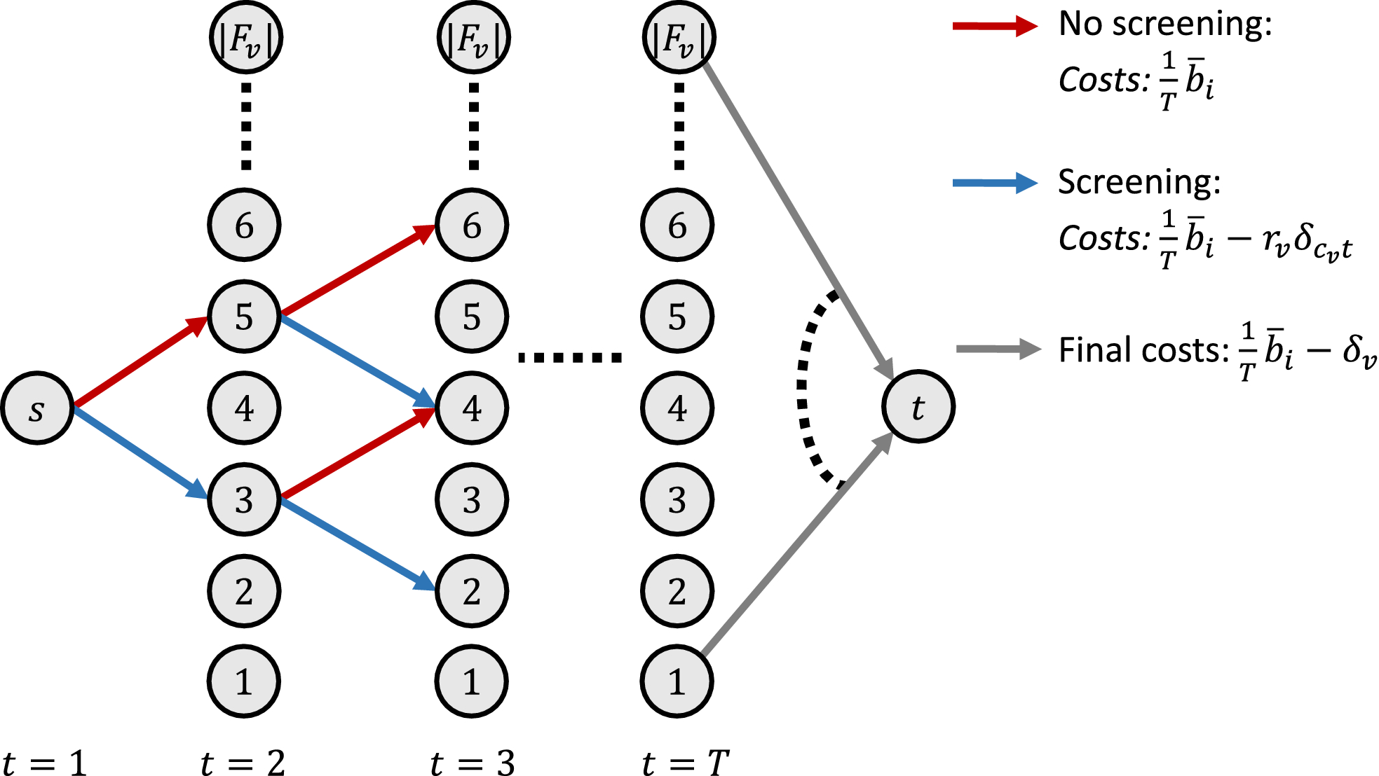
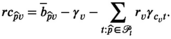
Graph Used to Solve the Pricing Problem for Village v as a Shortest Path Problem [Color figure can be viewed at
It can easily be verified that the length of a given s − t path provides a lower bound on the reduced costs of the corresponding visit pattern. Consequently, the shortest path obtained for any discretization 

Convergence of the algorithm is again guaranteed by the observation that the algorithm terminates as soon as the same path is encountered for the second time, and the number of possible paths is finite. Optimality is guaranteed by the observation that the length of the shortest path found equals the reduced costs of the corresponding visit pattern. Since the length of each alternative path provides a lower bound on their respective corresponding patterns, there is no alternative pattern having lower reduced costs.
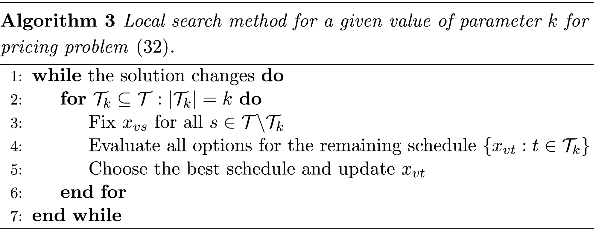
The idea behind the local search method is to repeatedly fix the schedule for village v for T − k planning periods and to optimize the schedule for the remaining periods by enumerating all options. We do so for k = 1 until the algorithm converges and proceed with k = 2 afterwards. For a given value of parameter k, the algorithm is explained below. As with the iterated local optimization method, we run the algorithm twice, using starting solutions 

Iterated Local Optimization
For a given planning period t and solution (


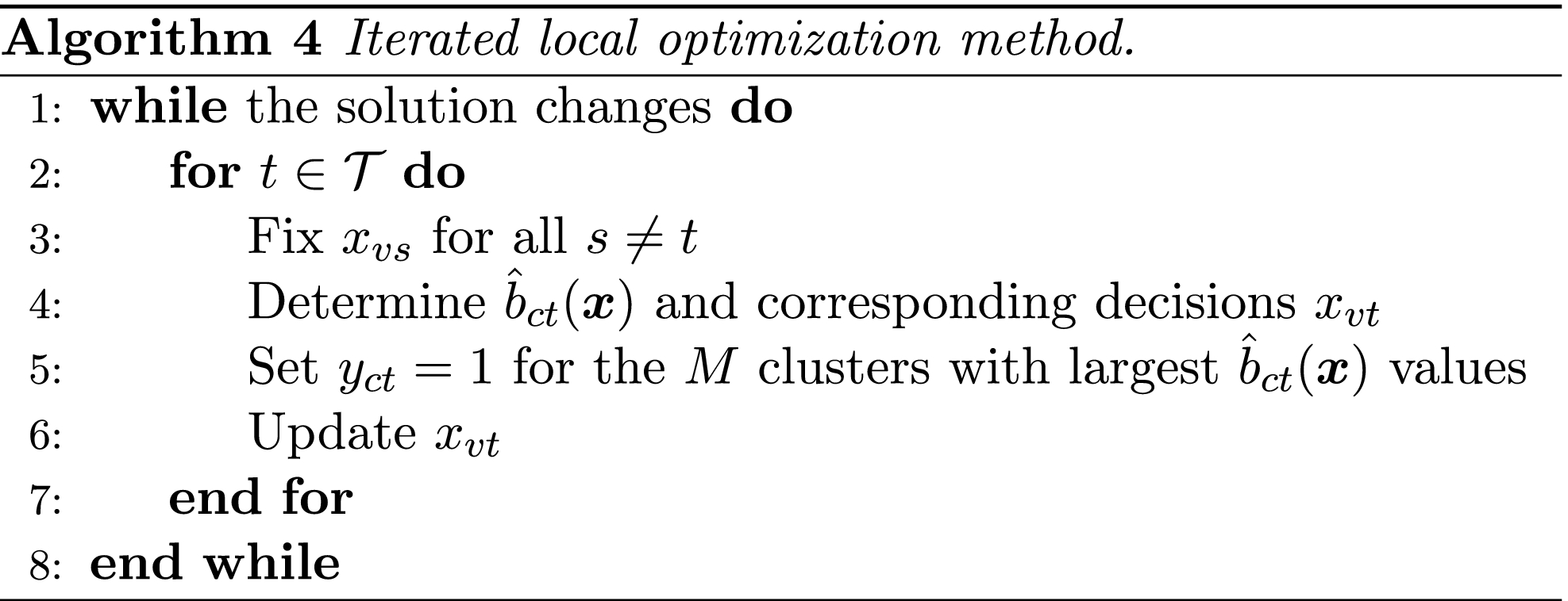
Determining 


Results on Case Study Variants
Table C1 describes results for three variants of the baseline case. In the first variant, which we refer to as Concentrated Cases, K v has been randomly generated from a U‐squared distribution with offset parameter α = 0.00237442 and vertical scale parameter β = 8.580473. The mean of this function is the same as the mean of the function used for the baseline case. The WorldPop variant uses 100 meter resolution population estimates from the WorldPop database (Tatem et al. 2007). Population of village v is estimated as the total population of grid cells within a 3.5 km radius. We fitted this radius by comparing the resulting average estimated population with the average population in the baseline case. Finally, the Random Clustering variant randomly assigns villages to the six clusters, while keeping the number of villages per cluster equal.
Average and Final (end of planning horizon of 36 months) Expected Number of People Infected in the 240 Villages for the Optimized Schedule and the Schedules Following from the Planning Policies, for the three Variants of the Baseline Case
We next assess the impact of excluding villages on our results. Specifically, we randomly select 10% of the villages to be removed from the baseline case, apply the policies, and determine the resulting expected average prevalence levels. We repeat this process 100 times. The following table describes the average and maximum optimality gap for the policies. It shows that the gaps are hardly affected and our general conclusions remain valid: Max Cases and Prevalence Increase yield near optimal decisions and the former slightly outperforms the latter Table C2.
Average and Maximum Optimality Gap when Excluding 10% of the Villages from the Baseline Case, Based on 100 Random Draws
Table of Notation
Key Notation