Sage Journals: Discover world-class research

Abstract

Recent advancements in Information Technology have provided an opportunity to significantly improve the effectiveness of inventory systems. The use of in‐cycle demand information enables faster reaction to demand fluctuations. In particular, for the newsvendor (NV) system, we exploit the newly available data to perform an additional review (AR) of inventory at an endogenously determined, a priori set time during the sales period, and perform an additional replenishment if necessary. We implemented our innovative model at a market‐leading media group. The results of the initial pilot were dramatic, indicating that the proposed model achieves an increase of 4%–24% in profits compared to the policy before implementation. As a result, the company started following the proposed model for all their printed magazines and observed a significant reduction in operational costs. In a generalized setting, we provide a tractable search‐based optimization algorithm, based on the problem's structural properties, for determining the optimal initial quantity, AR timing, and quantity to restock at that time. Based on these theoretical results, we propose a simple heuristic that can be used for many practical situations including our implementation at Yedioth. Through a computational experiment, we show that our algorithm finds the optimal solution quickly and that the proposed heuristic performs well. We also provide additional insights into the problem—for instance, that our system exhibits properties similar to inventory pooling, provided that the demand rate is large enough.

Keywords

print industry newsvendor two phases additional review replenishment timing

Introduction

Two major changes have affected supply chain management in recent years. The first is increased product variety accompanied by a shortening of product lifecycles. This combination has led to short‐term, highly uncertain demand profiles, making single‐period inventory models particularly relevant and widely used.

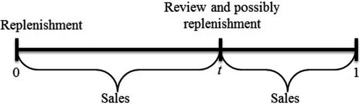
The second change is the recent advancements in Information Technology, such as Electronic Data Interchange (EDI) systems and Radio Frequency Identification (RFID) tags, which provide decision makers with extensive, accurate, and often real‐time, data. Wisely used, this newly available data can assist in improving the performance of the supply chain by reducing operational costs. For single‐period systems, such as the newsvendor (NV) system, one way to leverage this new information is to perform an additional review (AR) and possibly restock at an endogenously determined, a priori set time during the sales period, essentially creating two phases. Our goal is to leverage the available in‐cycle sales information to react to and address demand fluctuations. Whenever the words “replenishment” or “lotsizing” are used in this work, they equally refer to production or procurement. To clarify the problem setting, consider the following example.

A representative example of the print industry, and the motivating real‐world business case for this work, is Yedioth Group, the largest media group in Israel. Its distribution channel that is relevant to the current work includes around 8000 competing retailers. According to a common policy in the print industry, all lotsizing decisions are made solely by Yedioth and not by the retailers. This is due to the contractual mechanism and power relationship between the two parties. At the end of the sales period, excess copies are collected and retailers are fully refunded for unsold copies. In this way, all the surplus risk is borne by Yedioth, and the trade‐off faced by Yedioth for each retailer independently is captured by the standard NV problem. Yedioth uses an EDI system as well as RFID technology to monitor the sales of its print products at the points‐of‐sale (see, e.g., Avrahami et al. 2014). Thus, in‐cycle demand information is available at Yedioth virtually at any time. Moreover, it is possible to have an additional printing run during the sales period, provided that capacity is reserved well in advance. Once capacity has been reserved for the production of a certain print product, the actual quantity to be printed is flexible. Dynamic capacity allocation is not possible due to the printing facilities being shared by multiple products. Moreover, dynamic capacity allocation would have limited or no benefit due to the need of Yedioth's salespersons to commit to a schedule to visit the retailers at the beginning of the month.

Yedioth's situation is typical in the print industry where companies face ever‐growing competition from Internet‐based content. To survive and make a profit, the industry must streamline and reduce operational costs associated with print products. Thus, before the sales period begins, a printing house can decide that at a certain point during the period, after obtaining partial sales information, it may print and distribute another batch of the same product to meet the expected demand during the rest of the period. Due to the nature and sales profile of these products, the print industry fits very well into the newsvendor framework. Unmet demand is lost, surplus inventory is scrapped at the end of the period or is redirected to a secondary sales channel, and there is no holding cost during the period. In case of double‐printing and distribution, the most substantial part of the fixed production cost, that is, preparing the specially produced aluminum printing plates, is not incurred for the second production since these remain from the initial production. Because the printing process is considerably faster than the demand rate, the lead time is considered negligible and additional review and production are easily implementable. The costs associated with the distribution include mainly fuel, but the sales agents typically visit the retailers once more during the sales period anyway for purposes of promotion, advertisement, receiving payment, negotiations, and so on. The days of the additional visit are usually flexible, but must be prearranged for a few reasons. First, the retailers expect to know when the sales agent is coming. Second, the sales agents need to plan these visits among their other activities. Finally, for logistical efficiency, these additional visits need to be on the same day for geographically close retailers.

We model the problem as a stochastic planning problem with recourse and simultaneously optimize the initial order quantity, the timing of the AR, and the quantity to restock at that time. As verified numerous times in the literature, a correctly selected AR timing positively affects system performance compared to an arbitrarily selected one (Erkip 1984, van der Heijden 1999, Jönsson and Silver 1987, McGavin et al. 1993, Smirnov et al. 2021). These studies provide motivation for finding the optimal AR timing in the current work. As discussed in section 4, optimization over time is a complicating factor.

The AR timing in this work is endogenous but must be set before the start of the period. The order quantity at the time of the AR, however, is determined based on in‐cycle demand information. The reason for investigating this type of policy is two‐fold: first, in many industries, production facilities and resources are shared by multiple products. In this way, while the timing of the AR and production is potentially flexible, one must reserve production capacity in advance. Otherwise, the resources are likely to be occupied at the desired time of the additional replenishment. Second, as explained earlier, visits for an additional distribution generally cannot be carried out spontaneously due to other commitments of the sales agents.

The remainder of this study is organized as follows. In section 2, we review the relevant literature. In section 3, we provide the problem description and introduce the notation. In section 4, we analyze the problem and derive structural properties. In section 5, we develop our solution algorithm and section 5.1 presents a simple and practical heuristic. In section 6, we report on a computational experiment and discuss its results. In section 7, we report on the implementation of our model at Yedioth and the savings achieved. We conclude the work in section 8. All proofs appear in the online appendix.

Literature Review

Our work is related to two branches of research, namely, the two‐phase single‐retailer NV problem (e.g., Bulinskaya 1964), and determining the optimal review timing in a stochastic inventory system.

The two‐phase single‐retailer NV problem has been examined in the literature in several contexts such as operational constraints (e.g., Fisher and Raman 1996), forecast updating (e.g., Cachon and Swinney 2009, 2011, Choi et al. 2003), and supply chain coordination (e.g., Donohue 2000, Linh and Hong 2009). These studies utilize the fact that at the point of the AR, demand has been partially revealed. A more general setting includes multiple phases with a replenishment opportunity before each phase begins, and is not limited to a single retailer. The approach usually applied to this kind of problem is stochastic dynamic programming (e.g., Avrahami et al. 2014, Crowston et al. 1973, Nambiar et al. 2020), sometimes combined with Bayesian information updating (Eppen and Iyer 1997, Murray Jr. and Silver 1966). Most of the studies perform forecast updating, an issue not addressed in the current work. In contrast, our work optimizes the AR timing, an issue not considered in these papers.

Determining the optimal review or reorder timing in a stochastic inventory system is a problem addressed in various settings, including multiple periods, echelons or retailers (e.g., Liu and Song 2012, Rao 2003, Shang et al. 2015, Wang 2013, Wang and Axsäter 2013, Wang and Tomlin 2009). Some of the above studies involve lotsizing decisions in addition to timing decisions, and in others, optimization over timing is numerical. Our study, in contrast, simultaneously addresses both lotsizing and AR timing decisions in a single‐period setting with two ordering opportunities.

Closely related to our work is that of Milner and Kouvelis (2005), who study the value of order quantity and reorder timing flexibility in a single‐retailer, single‐period setting with two ordering opportunities. Aside from differences in the cost structure and demand processes, our work differs in several meaningful ways. We analyze the structure of the objective function in all decision variables. As a result, our algorithm always terminates with an optimal solution. In several cases, Milner and Kouvelis (2005) rely on a numerical search in a space whose structure is unknown. Milner and Kouvelis (2005) consider four ordering policies. We consider mainly one ordering policy that is similar to Milner and Kouvelis (2005)'s “quantity flexible” ordering policy (i.e., the reorder timing is fixed and the quantity of the second order is determined using in‐cycle demand information). Moreover, we propose a simple and practical heuristic that performs very well and numerically investigate alternate ordering policies. Finally, we justify our model by a real‐world business case and report on its implementation at a large printing house, including handling real sales data.

Problem Statement

Our focus in this study is Yedioth. In order to address Yedioth's printing decisions, however, we first model a slightly more general problem which lends itself to analysis and the development of effective and efficient algorithms for obtaining solutions. After computationally investigating our algorithms, we return to the case of Yedioth and show how our work has had a meaningful impact.

Planning Horizon and Demand Process

We consider a finite planning horizon, time‐scaled to the interval [0, 1]. The horizon consists of a single sales period, long enough to enable a meaningful division into two parts, [0, t] and [t,1], which we refer to as phases. Product units are discrete and demand follows a homogeneous Poisson counting process, N _t ≥ 0, with a constant arrival rate λ, an assumption that both reflects typical customer arrival and is standard in the literature. We define

N_{t_{1}, t_{2}} \equiv N_{t_{2}} - N_{t_{1}}

and use

N_{0, t}

and

N_{t, 1}

hereafter. By definition, N _0,0 = N _1,1≡0. Demand has realization n in the first phase and m in the second phase.

By definition, demand in the first phase follows a Poisson distribution with parameter λt, while demand in the second phase follows a Poisson distribution with parameter λ(1−t). It should be noted that for the example of Yedioth, the company experts found no correlation between the demand at the beginning of the sales period and the demand at its end. We confirm this by our own correlation analysis; see section 7.2.

Order of Events and Cost Structure

Prior to describing the order of events and cost structure, we introduce some basic notation. We define z ⁺≡max{z,0} and z ⁻≡max{−z,0}. We use Δ to denote a difference and z ^* to denote the optimal value of z. We use

\bar{z}

( z ) to denote an upper (lower) bound on z. We define

E_{Z}

as the expectation with respect to the random variable Z.

Before the initial ordering decision, the stock level at the single retailer we consider is zero. Lead time and fixed replenishment costs are negligible.

At time 0, the system orders a quantity Q ₀ at a unit cost of c ₁, thus incurring an initial variable ordering cost of c ₁ Q ₀, and items are received. Subsequently, the sales period starts and demand gradually unfolds. V is the unit selling price. Contrary to the standard NV problem where no AR takes place, the stock level is reviewed at an endogenously determined a priori set time t, and an additional replenishment is (possibly) performed at a unit cost of c ₂ ≥ c ₁. The AR can be performed at any moment throughout the sales period. We remind the reader, however, that the AR timing must be determined before the period begins, as the salespersons’ visits to the retailers must be scheduled in advance. By time t, the system receives a revenue of

V min {Q_{0}, N_{0, t}}

. If there were lost sales before the AR, a penalty cost of p per unit is charged for them. Hence, the lost sales costs for the first phase are

p {(N_{0, t} - Q_{0})}^{+}

. No holding costs are incurred at the time of the AR.

Depending on the realization of

N_{0, t}

, a replenishment may be performed at time t. The amount restocked is

Q (t, {(Q_{0} - N_{0, t})}^{+})

, resulting in a cost of

c_{2} Q (t, {(Q_{0} - N_{0, t})}^{+})

. The second phase starts with an actual stock level of

{(Q_{0} - N_{0, t})}^{+} + Q (t, {(Q_{0} - N_{0, t})}^{+})

, comprising the surplus from the first phase and the quantity replenished at time t, each of which might be zero. In fact, the NV structure of the problem faced at time t implies a base‐stock policy for the second phase. We denote the order‐up‐to level by S(t). Given n arrivals in the first phase, A(t) = (Q ₀−n)⁺+Q(t,(Q ₀−n)⁺) is the actual inventory at time t, and we note that A(t) only becomes known at time t.

After the AR, sales continue and result in a revenue of

V min {{(Q_{0} - N_{0, t})}^{+} + Q (t, {(Q_{0} - N_{0, t})}^{+}), N_{t, 1}}

for the second phase. At the end of the period (time 1), the system incurs either disposal costs of h per unit for surplus inventory or penalty costs (again, p per unit) for lost sales in the second phase. This results in a cost of

h {({(Q_{0} - N_{0, t})}^{+} + Q (t, {(Q_{0} - N_{0, t})}^{+}) - N_{t, 1})}^{+} + p {(N_{t, 1} - {(Q_{0} - N_{0, t})}^{+} - Q (t, {(Q_{0} - N_{0, t})}^{+}))}^{+}

for the second phase. Figure 1 depicts the order of events in the proposed system.

Figure 1

Order of Events in the Proposed System

We assume c ₂ ≥ c ₁ as we expect this relation to hold for most practical situations. We conjecture that without this assumption, all results hold or can be adjusted with minor modifications. Moreover, in most cases, including in the bakery and printing house examples, the relation is c ₁ = c ₂. A situation of c ₂ > c ₁ might occur if, for instance, outsourcing or emergency production is used for the additional replenishment. To avoid uninteresting situations, we make the standard assumptions p+V > c ₂ and c ₁ > −h.

We use the ordered pair

(Q_{0}, t)

to represent a solution. π _t is the expected profit for the second phase, while π ₀ is the expected profit for the entire period. Our objective is to select Q ₀ and t to maximize

π_{0} (Q_{0}, t)

. As we will see, the replenishment policy at the time of the AR is uniquely determined by t. Below we summarize the notation that is introduced in this section (additional notation will be introduced when first used).

c ₁	Unit ordering and replenishment cost at time 0
c ₂	Unit ordering and replenishment cost at the time of the AR, c ₂ ≥ c ₁
V	Unit selling price
h	Unit disposal cost at the end of the period
p	Unit penalty cost for lost sales; the same for both phases
$N_{0, t} \geq 0$	Random variable with mean λt resulting from a Poisson counting process representing demand during a time interval of length t
n	Realization of demand in the first phase
m	Realization of demand in the second phase
t	AR timing, t ∈ [0,1]
Q ₀	Quantity ordered at time 0
$Q (t, {(Q_{0} - N_{0, t})}^{+})$	Quantity replenished at time t, t ∈ [0,1], when the inventory level is ${(Q_{0} - N_{0, t})}^{+}$
S(t)	Order‐up‐to level at time t, t ∈ [0,1], with a unit cost of c ₂
A(t)	Actual stock level at time t after the AR, given n arrivals in the first phase
$(Q_{0}, t)$	Representation of a solution
π _t	Expected profit for the second phase
π ₀	Expected profit for the entire period consisting of both phases

Analysis

Suppose for now that t is fixed and consider the problem faced at time t. This problem is a building block in the problem for the entire period.

Observation 1

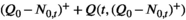
Given t ∈ [0, 1], if Q ₀ units are ordered at time 0 and there are n arrivals before time t, the expected profit of the second phase, [t,1], is the standard NV expected profit, that is,

V E_{N_{t, 1}} [min {N_{t, 1}, A (t)}] - c_{2} (A (t) - {(Q_{0} - n)}^{+}) - h E_{N_{t, 1}} [{(A (t) - N_{t, 1})}^{+}] - p E_{N_{t, 1}} [{(N_{t, 1} - A (t))}^{+}]

Observation 1 implies the following result (

N

is the set of natural numbers, including zero).

Proposition 1

Given t ∈ [0,1], the expected profit of the second phase is discrete concave in S(t) and it holds that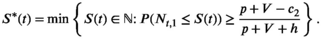

S^{*} (t) = min \{S (t) \in N : P (N_{t, 1} \leq S (t)) \geq \frac{p + V - c_{2}}{p + V + h}\} .

Moreover, given t ∈ [0,1], S ^*(t) is also the optimal order‐up‐to level at the time of the AR for our proposed system.

Constraining S(t) = 0, or setting t = 0 or t = 1 reduces the problem to the simple NV system. The proposed system clearly has an expected profit no less than a simple NV system solved at time 0. Since both probabilities

P (N_{t, 1} \leq x)

and

P (N_{0, t} \geq x)

are increasing in t for any x ≥ 0, we have the following observation, which will be useful throughout the study.

Observation 2

For all

t_{1}, t_{2} \in [0, 1]

such that

t_{1} < t_{2}

, it holds that

S^{*} (t_{1}) \geq S^{*} (t_{2})

Objective Function

As mentioned in section 1, optimization with respect to t is a complicating factor for the model. It means adding a continuous decision variable to a problem in which the other decision variables are discrete, thus creating a mixed discrete‐continuous optimization problem. Additionally, and possibly for the same reason, having timing as a decision variable is nonstandard in the literature of stochastic planning problems with recourse.

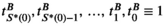
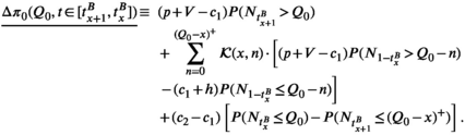
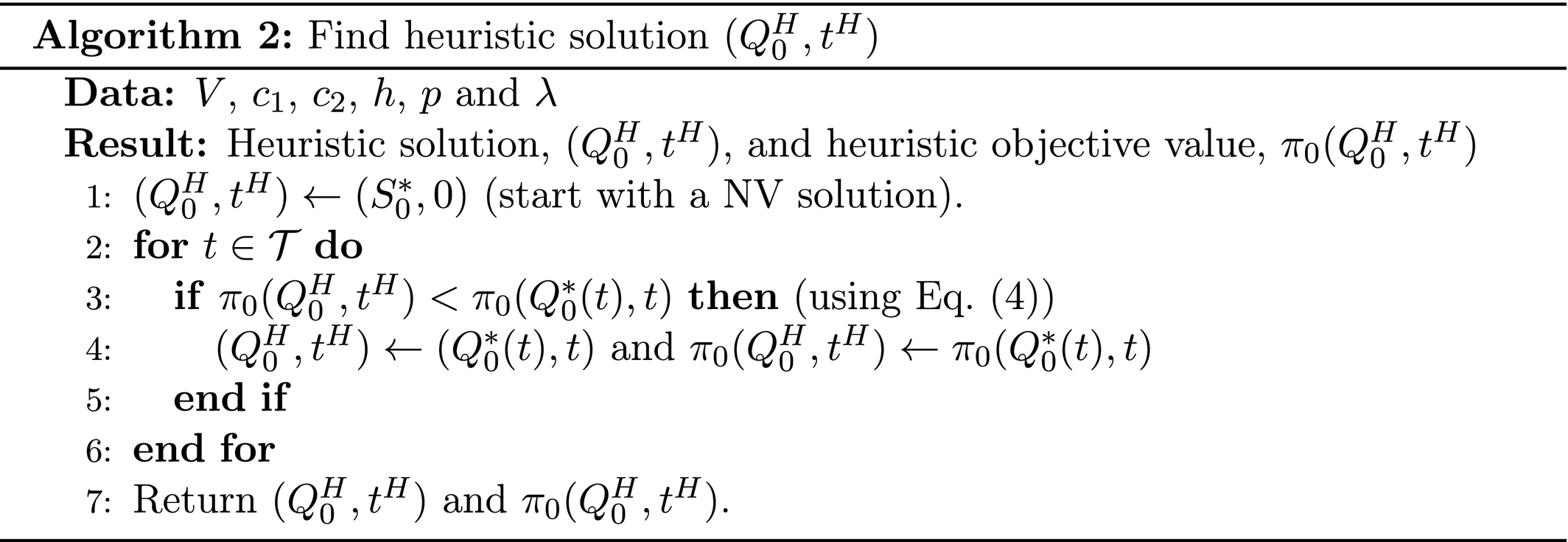
In its most general form, our objective—the expected profit for the period (π ₀)—is a function of three decision variables, namely the quantity to order at time 0 (Q ₀), the AR timing (t) and the order‐up‐to level at the time of the AR (S(t)).

Conditioning on the number of arrivals in the first phase and on the number of arrivals in the second phase, and removing the dependence between the AR timing and the order‐up‐to level at the time of the AR, the expected profit for the period is: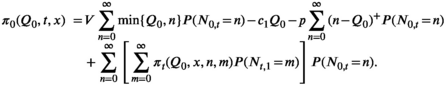

\begin{matrix} π_{0} (Q_{0}, t, x) & = V \sum_{n = 0}^{\infty} min {Q_{0}, n} P (N_{0, t} = n) - c_{1} Q_{0} - p \sum_{n = 0}^{\infty} {(n - Q_{0})}^{+} P (N_{0, t} = n) \\ + \sum_{n = 0}^{\infty} [\sum_{m = 0}^{\infty} π_{t} (Q_{0}, x, n, m) P (N_{t, 1} = m)] P (N_{0, t} = n) . \end{matrix}

The expression in square brackets in Equation (2) reflects the profit‐to‐go, where:

\begin{matrix} π_{t} (Q_{0}, x, n, m) & = V min \{max {x, {(Q_{0} - n)}^{+}}, m\} - c_{2} (max {x, {(Q_{0} - n)}^{+}} - {(Q_{0} - n)}^{+}) \\ - h {(max {x, {(Q_{0} - n)}^{+}} - m)}^{+} - p {(m - max {x, {(Q_{0} - n)}^{+}})}^{+} . \end{matrix}

To gain insight into the problem, let us examine Figure 2a, which, for a particular problem instance, depicts π ₀ as a function of t for a fixed Q ₀ = 16 for various order‐up‐to levels. Each curve corresponds to an order‐up‐to level x (

x \in {0, \dots, S^{*} (0)}

). For example, the leftmost curve in Figure 2a represents the function π ₀(16, t, 16), the next curve to the right represents the function π ₀(16, t, 15), and so on. The horizontal line in Figure 2a represents the function π ₀(16, t, 0).

Figure 2

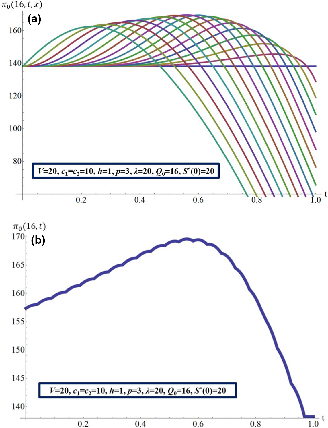
Expected Profit as a Function of t for a Fixed Q ₀ = 16 [Color figure can be viewed at wileyonlinelibrary.com]

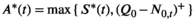
Proposition 1 established that the optimal order‐up‐to level at time t depends only on t; thus, the dimension of the problem can be reduced from three variables to two variables by defining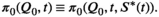

π_{0} (Q_{0}, t) \equiv π_{0} (Q_{0}, t, S^{*} (t)) .

Graphically, this means that in Figure 2a, we select the top curve for every possible AR timing, thereby obtaining a “pseudo‐cloud‐shaped” curve (see, e.g., Liu and Song 2012, where they discuss a cloud‐shaped curve); see Figure 2b.

In the problem we investigate, however, Q ₀ is not fixed. We now formulate our objective function as a stochastic planning problem with recourse: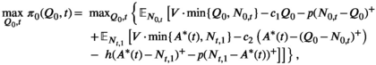

\begin{matrix} max_{Q_{0}, t} π_{0} (Q_{0}, t) = & {max}_{Q_{0}, t} \{E_{N_{0, t}} [V \cdot min {Q_{0}, N_{0, t}} - c_{1} Q_{0} - p {(N_{0, t} - Q_{0})}^{+} \\ + E_{N_{t, 1}} [V \cdot min {A^{*} (t), N_{t, 1}} - c_{2} (A^{*} (t) - {(Q_{0} - N_{0, t})}^{+}) \\ - h {(A^{*} (t) - N_{t, 1})}^{+} - p {(N_{t, 1} - A^{*} (t))}^{+}]]\}, \end{matrix}

where

Q_{0} \in N

and t ∈ [0,1] are the first‐stage decision variables (note that having the timing of the recourse as a decision variable is nonstandard in stochastic dynamic programming), and

A^{*} (t) = max {S^{*} (t), {(Q_{0} - N_{0, t})}^{+}}

is the recourse action. The expected profit function is thus a collection of pseudo‐cloud‐shaped curves of the type presented in Figure 2, with each curve corresponding to a particular value of Q ₀.

Breakpoints

Let us consider the timing of the AR. As the AR is performed later in the planning horizon, less inventory will be needed in the second phase (Observation 2). When the AR is performed close to time 1, one would prefer not to restock. Since demand is integral, S ^*(t) is a decreasing step function of t with a step height of one. For an illustrative example of the impact of t on S ^*(t), see Figure 3.

Figure 3

Illustration of the Impact of t on S ^*(t) When

S^{*} (0) = 8

[Color figure can be viewed at wileyonlinelibrary.com]

A breakpoint

t_{x}^{B}

is a point in the time dimension (t ∈ [0,1]) at which one changes the optimal order‐up‐to level. By definition, we add two extreme breakpoints, t = 0 and t = 1. Thus, the breakpoints create

S^{*} (0) + 1

different intervals, each characterized by a different optimal order‐up‐to level. Note that these breakpoints are independent of Q ₀. Each “piece” of the pseudo‐cloud‐shaped function depicted in Figure 2b corresponds to the time interval between two consecutive breakpoints.

Definition 1

For all

x = 1, \dots, S^{*} (0)

, the breakpoint associated with ordering up to x units at the time of the AR is defined as

t_{x}^{B} = {t \geq 0 : P (N_{t, 1} < x) = (p + V - c_{2}) / (p + V + h)}

The sequence of breakpoints is thus

t_{S^{*} (0) + 1}^{B} \equiv 0

t_{S^{*} (0)}^{B}, t_{S^{*} (0) - 1}^{B}, \dots, t_{1}^{B}, t_{0}^{B} \equiv 1

. We sometimes refer to the time interval

[t_{x + 1}^{B}, t_{x}^{B}]

as interval x. We also note that

Proposition 2

When

t = t_{x}^{B}

x = 1, \dots, S^{*} (0)

, both x and x−1 are optimal order‐up‐to levels.

Bounds on the Initial Order Quantity,
$Q_{0}^{*}$

In this section, we establish upper and lower bounds on the optimal quantity to order at time 0, when the AR timing lies between

t_{x + 1}^{B}

and

t_{x}^{B}

. We denote them by

Q_{0}^{* U} (x)

and

Q_{0}^{* L} (x)

, respectively. These bounds are needed for our search‐based solution algorithm (section 5). The following lemma will be useful in establishing these bounds, and in optimizing with respect to quantity in general.

Lemma 1

Given t ∈ [0,1],

π_{0} (Q_{0}, t)

is discrete concave with respect to Q ₀, and thus

Q_{0}^{*} (t)

is the smallest value for which

\begin{matrix} Δ π_{0} (Q_{0}, t) = & (p + V - c_{1}) P (N_{0, t} > Q_{0}) \\ + (c_{2} - c_{1}) P ({(Q_{0} - S^{*} (t))}^{+} < N_{0, t} \leq Q_{0}) \\ + \sum_{n = 0}^{{(Q_{0} - S^{*} (t))}^{+}} P (N_{0, t} = n) [(p + V - c_{1}) P (N_{t, 1} > Q_{0} - n) - (c_{1} + h) P (N_{t, 1} \leq Q_{0} - n)] . \end{matrix}

is nonpositive.

Defining

S_{0}^{*}

as the optimal NV quantity at time 0 (at a unit cost of c ₁) and

K (x, n)

as the maximum of

P (N_{0, t} = n)

over the interval

[t_{x + 1}^{B}, t_{x}^{B}]

(see Lemma 3 in Appendix B for an explicit expression for

K (x, n)

), the bounds on

Q_{0}^{*}

are:

Theorem 1

An upper bound and lower bound on

Q_{0}^{*}

for all

t \in [t_{x + 1}^{B}, t_{x}^{B}]

are, respectively, as follows:

Q_{0}^{* U} (x) = min {S_{0}^{*}, min {Q_{0} \in N : \bar{Δ π_{0} (Q_{0}, t \in [t_{x + 1}^{B}, t_{x}^{B}])} \leq 0}}

, where

\begin{matrix} \bar{Δ π_{0} (Q_{0}, t \in [t_{x + 1}^{B}, t_{x}^{B}])} \equiv & (p + V - c_{1}) P (N_{t_{x}^{B}} > Q_{0}) + \sum_{n = 0}^{{(Q_{0} - x)}^{+}} \{min {P (N_{t_{x + 1}^{B}} = n), P (N_{t_{x}^{B}} = n)} \\ \cdot [(p + V - c_{1}) P (N_{1 - t_{x + 1}^{B}} > Q_{0} - n) - (c_{1} + h) P (N_{1 - t_{x + 1}^{B}} \leq Q_{0} - n)]\} \\ + (c_{2} - c_{1}) [P (N_{t_{x + 1}^{B}} \leq Q_{0}) - P (N_{t_{x}^{B}} \leq {(Q_{0} - x)}^{+})] . \end{matrix}

Q_{0}^{* L} (x) = max {x, min {Q_{0} \in N : \underset{̲}{Δ π_{0} (Q_{0}, t \in [t_{x + 1}^{B}, t_{x}^{B}])} \leq 0}}

, where

\begin{matrix} \underset{̲}{Δ π_{0} (Q_{0}, t \in [t_{x + 1}^{B}, t_{x}^{B}])} \equiv & (p + V - c_{1}) P (N_{t_{x + 1}^{B}} > Q_{0}) \\ + \sum_{n = 0}^{{(Q_{0} - x)}^{+}} K (x, n) \cdot [(p + V - c_{1}) P (N_{1 - t_{x}^{B}} > Q_{0} - n) \\ - (c_{1} + h) P (N_{1 - t_{x}^{B}} \leq Q_{0} - n)] \\ + (c_{2} - c_{1}) [P (N_{t_{x}^{B}} \leq Q_{0}) - P (N_{t_{x + 1}^{B}} \leq {(Q_{0} - x)}^{+})] . \end{matrix}

The intuition underlying the result

Q_{0}^{*} \leq S_{0}^{*}

is that since there is a chance to restock later in the period, fewer units are needed at time zero. Note that all other bounds in this section are interval‐dependent.

Analysis with Respect to the Additional Review Timing

In this section, we provide an analysis of the expected profit as a function of the AR timing (t) for given Q ₀ and x. The results of this analysis are used later in our solution algorithm (section 5). The following lemma is useful for identifying structural properties of the problem such as unimodaity between breakpoints and breakpoints not being optimal, as well as for developing a bound on the expected profit between breakpoints:

Lemma 2

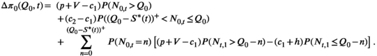
Given Q ₀ and x, the derivative of the expected profit for the period with respect to t is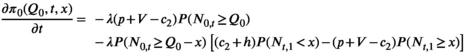

\begin{matrix} \frac{\partial π_{0} (Q_{0}, t, x)}{\partial t} = & - λ (p + V - c_{2}) P (N_{0, t} \geq Q_{0}) \\ - λ P (N_{0, t} \geq Q_{0} - x) [(c_{2} + h) P (N_{t, 1} < x) - (p + V - c_{2}) P (N_{t, 1} \geq x)] \end{matrix}

Returning to the pseudo‐cloud‐shaped function (see Figure 2b), we note that for AR timings other than the breakpoints, it holds that

\partial π_{0} (Q_{0}, t) / \partial t = \partial π_{0} (Q_{0}, t, x) / \partial t

. Additionally, we note that

\partial π_{0} (Q_{0}, t) / \partial t

is undefined at the breakpoints because two different order‐up‐to levels are used to the left and right of breakpoint. To calculate the left and right derivatives, respectively, at a breakpoint

t_{x}^{B}

, we take the limit of Equation (9) evaluated at order‐up‐to levels x and x−1, respectively. The following Theorem allows us to eliminate the breakpoints from further consideration.

Theorem 2

No breakpoint

t_{x}^{B}

(

x = 1, \dots, S^{*} (0)

) is optimal.

A key result that is used in our solution algorithm (section 5) concerns the function's piecewise behavior. Despite the fact that

π_{0} (Q_{0}, t)

appears, for most instances, to be piecewise concave, we have found examples for which this is not the case. Nevertheless, we have:

Theorem 3

Given Q ₀ and x, Q ₀ ≥ x,

π_{0} (Q_{0}, t, x)

is strictly unimodal in t for x > 0 and constant for x = 0.

Theorem 3 implies that

π_{0} (Q_{0}, t)

is piecewise‐strictly pseudo‐concave in t for

t < t_{1}^{B}

and is constant for

t > t_{1}^{B}

. Accordingly, the expected profit can be optimized interval‐wise with respect to t (for all x and for all Q ₀) and the global maximum can be selected by comparing values from a finite set. Our final algorithm (section 5) uses this fact along with Theorem 4. Theorem 3 also allows us to eliminate intervals from our search space according to the following observation.

Observation 3

For a given Q ₀, if

{lim}_{t \to t_{x + 1}^{B +}} \partial π_{0} (Q_{0}, t) / \partial t < 0

{lim}_{t \to t_{x}^{B -}} \partial π_{0} (Q_{0}, t) / \partial t > 0

(

x \in {0, \dots, S^{*} (0)}

), the global maximizer of

π_{0} (Q_{0}, t)

is not found in the interval

[t_{x + 1}^{B}, t_{x}^{B}]

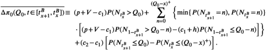
Given Q ₀ and x, we derive an upper bound on the expected profit in the interval

[t_{x + 1}^{B}, t_{x}^{B}]

. This bound is utilized in our solution algorithm (section 5) to eliminate intervals from consideration. The bound on the expected profit uses bounds on the derivative with respect to the time domain, and is illustrated in Figure 4.

Figure 4

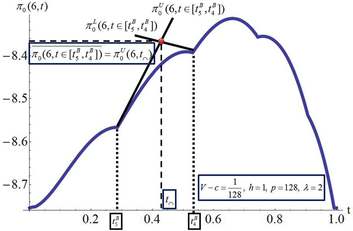
Illustration of the Upper Bound on the Expected Profit from Theorem 4 [Color figure can be viewed at wileyonlinelibrary.com]

Theorem 4

Given Q ₀ and x, an upper bound on the expected profit over

[t_{x + 1}^{B}, t_{x}^{B}]

\bar{π_{0} (Q_{0}, t \in [t_{x + 1}^{B}, t_{x}^{B}])} \equiv π_{0} (Q_{0}, t_{x + 1}^{B}, x) + \bar{\partial π_{0} (Q_{0}, t \in [t_{x + 1}^{B}, t_{x}^{B}]) / \partial t} (t_{\cap} - t_{x + 1}^{B}),

where

t_{\cap} = \frac{\bar{\partial π_{0} (Q_{0}, t \in [t_{x + 1}^{B}, t_{x}^{B}]) / \partial t} \cdot t_{x + 1}^{B} - \underset{̲}{\partial π_{0} (Q_{0}, t \in [t_{x + 1}^{B}, t_{x}^{B}]) / \partial t} \cdot t_{x}^{B} + π_{0} (Q_{0}, t_{x}^{B}, x) - π_{0} (Q_{0}, t_{x + 1}^{B}, x)}{\bar{\partial π_{0} (Q_{0}, t \in [t_{x + 1}^{B}, t_{x}^{B}]) / \partial t} - \underset{̲}{\partial π_{0} (Q_{0}, t \in [t_{x + 1}^{B}, t_{x}^{B}]) / \partial t}},

\bar{\partial π_{0} (Q_{0}, t \in [t_{x + 1}^{B}, t_{x}^{B}]) / \partial t}

and

\underset{̲}{\partial π_{0} (Q_{0}, t \in [t_{x + 1}^{B}, t_{x}^{B}]) / \partial t}

are, respectively, upper and lower bounds on the derivative of

π_{0} (Q_{0}, t)

with respect to t over

[t_{x + 1}^{B}, t_{x}^{B}]

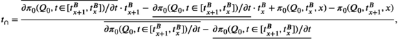
The reader is referred to Appendix B for expressions for

\bar{\partial π_{0} (Q_{0}, t \in [t_{x + 1}^{B}, t_{x}^{B}]) / \partial t}

and

\underset{̲}{\partial π_{0} (Q_{0}, t \in [t_{x + 1}^{B}, t_{x}^{B}]) / \partial t}

. They are derived similarly to the bounds in Eqs. 7 and 8.

Solution Algorithm

Our optimization algorithm (see Algorithm 1) begins by finding an initial candidate solution. Subsequently, it checks interval–initial quantity (IQ) pairs,

(x, Q_{0})

, and either finds a better solution or demonstrates that the IQ pair can be eliminated from consideration. We define

t_{(x, Q_{0})}^{s}

as the stationary point on the time domain associated with the IQ pair

(x, Q_{0})

, and

(Q_{0}, t \in [t_{x + 1}^{B}, t_{x}^{B}])

as the representation of a solution when

t \in [t_{x + 1}^{B}, t_{x}^{B}]

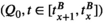
Note that at the end of the execution of Algorithm 1,

(Q_{0}^{*}, t^{*})

is an optimal solution, but during the execution of the algorithm, it is merely the best candidate solution found so far. We rely on Theorem 1 for setting the start and end values of the inner loop.

For each IQ pair

(x, Q_{0})

, we begin by applying various elimination tests, based on properties detailed and discussed in section 4. We begin with a pair of elimination tests based on Observation 3 (Lines 4–5). The next test (Lines 6–8) eliminates IQ pairs whose expected profit is too low compared to the current best candidate solution.

If an IQ pair is not eliminated, the first‐order condition is applied in that interval (Line 10) using Newton's method. Since

π_{0} (Q_{0}, t, x)

is strictly unimodal, if Newton's method converges, then it converges to the local maximum. Newton's method has the advantage of a quadratic convergence rate and little sensitivity to the selection of the initial point. If Newton's method fails to converge, one can use a golden section search instead. In a large experiment consisting of 2857 different problem instances, however, we observed that Newton's method always converged. For each IQ pair

(x, Q_{0})

, we could have skipped the elimination criteria and simply applied Newton's method for each interval, but this would have required considerably longer run times.

As stated above, Algorithm 1 begins by finding an initial candidate solution. The algorithm terminates with the optimal solution no matter what initial solution is used. This solution, however, does affect the execution time. Depending on the value of λ, we apply two different heuristics.

When λ is small (λ < 16), the optimization algorithm is extremely fast, hence we do not invest significant time in finding the initial solution. In this case, we use a heuristic rule inspired by McGavin et al. (1993), who, although addressing a different problem, heuristically divided the period into two phases of equal length. Thus, we set the initial AR timing to be 0.5 and optimize with respect to Q ₀ by enumerating all Q ₀'s starting with S ^*(0.5) until we find one for which Equation (6) is nonpositive (see Lemma 1).

For larger λ, it becomes worthwhile to invest effort in finding a good initial solution. Although the optimal solution is not found at a breakpoint (Theorem 2), for λ ≥ 16, we find a two‐dimensional locally optimal breakpoint as the initial candidate solution. We use alternating optimization, that is, starting with

Q_{0} = S^{*} (0)

, we alternately optimize over one of the decision variables while holding the other constant. The algorithm converges since the objective value increases at each step and there is a finite number of candidates.

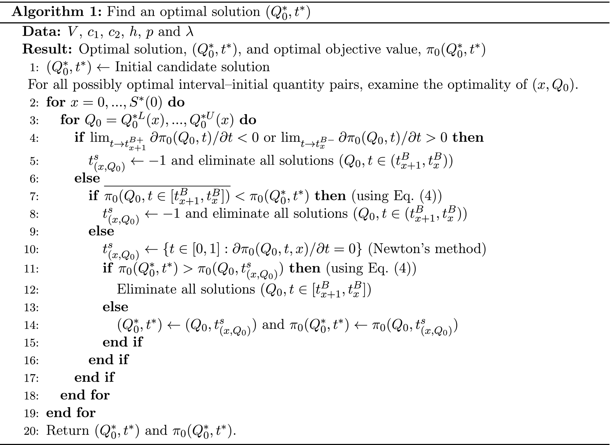
Discrete‐Time Heuristic

In many practical situations, there is a finite set of possible AR times. For such cases, we present a simple and useful heuristic, whose principle is enumerate the possible AR timings and, for each possible AR timing, optimize the initial quantity and the optimal order‐up‐to level. We define

T

as the set of all possible AR timings, and

(Q_{0}^{H}, t^{H})

as the heuristic solution after the termination of the heuristic algorithm and as a temporary solution otherwise. The heuristic algorithm is outlined in Algorithm 2 and tested at the end of section 6.

Computational Experiments

In this section, we report numerical results that provide insight beyond what can be seen from the analytical results, thus completing the picture of our system with an AR. Moreover, we demonstrate the speed of our algorithm.

We now examine what we believe to be the most interesting case, that is, c ₁ = c ₂≡c. Assuming the same unit ordering cost in both phases also enables us to reduce the number of parameters in our experiment to just two.

The expected profit for the period (Equation 5) for the case c ₁ = c ₂≡c can be rewritten as:

\begin{matrix} max_{Q_{0}, t} π_{0} (Q_{0}, t) = & (p + V + h) \cdot max_{Q_{0}, t} \{\frac{(V - c) λ}{p + V + h} - E_{N_{0, t}} [E_{N_{t, 1}} [{(A^{*} (t) - N_{t, 1})}^{+}]] \\ + \frac{p + V - c}{p + V + h} E_{N_{0, t}} [E_{N_{t, 1}} [A^{*} (t) - N_{t, 1}] - {(N_{0, t} - Q_{0})}^{+}]\} . \end{matrix}

Examining Equation (10), we get the following result.

Proposition 3

If the unit ordering cost is identical in both phases, the cost parameters (V, c, h and p) influence the optimal solution

(Q_{0}^{*}, t^{*})

only through the standard NV critical ratio (CR), (p+V−c)/(p+V+h).

By Proposition 3, each problem instance examined in the computational experiment is characterized by a combination of λ and a critical ratio, (p+V−c)/(p+V+h). Note that this result is similar to the result regarding the optimal order quantity in the standard NV problem.

Due to the fact that the expected profits of both the system with an AR and the NV system depend on V, c, h, and p (and not only on the critical ratio), we decided to compare problem instances using a unitless measure that depends solely on λ and the critical ratio. This measure, which we call PRUC (Percent Reduction in Uncertainty Cost), is defined as the portion of the costs due to uncertainty reduced by applying our AR model, relative to a system with perfect information.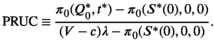

PRUC \equiv \frac{π_{0} (Q_{0}^{*}, t^{*}) - π_{0} (S^{*} (0), 0, 0)}{(V - c) λ - π_{0} (S^{*} (0), 0, 0)} .

Note that

π_{0} (S^{*} (0), 0, 0)

is the expected profit of the standard NV problem, and (V−c)λ is the profit if we knew the demand realization before ordering.

We conducted a full‐factorial experiment involving ten different values of λ and seven different values of the critical ratio, 70 instances in all. Specifically, we used λ = 2^k, k ∈ {0, 1, 2, 3, 4, 5, 6, 7, 8, 9} and (p+V−c)/(p+V+h) ∈ {0.05, 0.1, 0.3, 0.5, 0.7, 0.9, 0.95}.

In our implementation of the calculation of the objective function, we replaced the limits of the infinite sums (e.g.,

\sum_{n = 0}^{\infty}

) with two λ‐dependent expressions. For a Poisson distribution with a rate of λ, the smallest number of events considered is

max {⌊ λ - 5 \sqrt{λ} ⌋, 0}

, and the largest is

max {⌈ λ + 5 \sqrt{λ} ⌉, 20}

. The largest total probability thus ignored for all our runs is 4.977·10⁻⁶. The λ‐dependent limits of the sum contribute to the fact that the run time increases in λ.

Our results are reported in Table 1, we exclude critical ratios of 0.05 and 0.1 for conciseness as they do not affect our observations and conclusions. The first two columns of both sides show the parameters, λ and the CR. The next three columns present the optimal solutions, that is, providing the optimal initial order quantity, the optimal AR timing, and the optimal order‐up‐to level at the time of the AR. The sixth column contains the expected quantity ordered (EQO) for both phases (i.e., the optimal initial quantity plus the expected quantity replenished at the time of the AR). This quantity is given by

Q_{0}^{*} + S^{*} (t^{*}) P (N_{t^{*}} \geq Q_{0}^{*}) + \sum_{n = Q_{0}^{*} - S^{*} (t^{*})}^{Q_{0}^{*} - 1} P (N_{t^{*}} = n) [S^{*} (t^{*}) - (Q_{0}^{*} - n)]

. The seventh column provides the optimal solution of a standard NV problem with the same parameters. The rightmost column presents the PRUC under our two‐phase model.

Table 1

Results of the Computational Study and a Comparison to the Newsvendor Model

λ	CR	$Q_{0}^{*}$	$t^{*}$	$S^{} (t^{})$	EQO	$S^{*} (0)$	PRUC	λ	CR	$Q_{0}^{*}$	$t^{*}$	$S^{} (t^{})$	EQO	$S^{*} (0)$	PRUC
1	0.3	0	0.00	0	0	0	0.00%	32	0.3	26	0.66	9	30.1	29	32.4%
1	0.5	1	0.15	1	1.14	1	2.75%	32	0.5	28	0.68	10	32.1	32	34.3%
1	0.7	1	0.32	1	1.28	1	14.4%	32	0.7	30	0.70	11	33.9	35	35.8%
1	0.9	2	0.34	2	2.34	2	14.7%	32	0.9	33	0.72	13	36.6	39	37.3%
1	0.95	2	0.42	2	2.41	3	14.8%	32	0.95	34	0.70	15	38.0	42	37.6%
2	0.3	1	0.20	1	1.33	1	7.43%	64	0.3	54	0.71	16	61.6	60	39.8%
2	0.5	2	0.43	1	2.21	2	7.09%	64	0.5	57	0.73	17	64.1	64	41.2%
2	0.7	2	0.32	2	2.61	3	15.7%	64	0.7	60	0.75	18	66.5	68	42.2%
2	0.9	3	0.54	2	3.39	4	16.2%	64	0.9	64	0.75	21	70.1	74	43.2%
2	0.95	4	0.50	3	4.37	5	19.5%	64	0.95	66	0.76	22	71.7	77	43.3%
4	0.3	2	0.27	2	2.96	3	10.6%	128	0.3	112	0.77	26	126	122	46.7%
4	0.5	3	0.44	2	3.78	4	14.9%	128	0.5	116	0.78	28	128	128	47.7%
4	0.7	4	0.44	3	4.89	5	18.0%	128	0.7	120	0.79	29	131	134	48.5%
4	0.9	5	0.49	4	6.08	7	21.6%	128	0.9	125	0.80	32	135	143	49.1%
4	0.95	6	0.58	4	6.72	8	23.8%	128	0.95	128	0.80	34	138	147	49.1%
8	0.3	6	0.48	3	7.09	6	18.3%	256	0.3	231	0.82	42	252	247	53.2%
8	0.5	7	0.50	4	8.25	8	20.5%	256	0.5	237	0.83	43	256	256	54.0%
8	0.7	8	0.59	4	9.17	9	23.9%	256	0.7	242	0.84	45	260	264	54.5%
8	0.9	9	0.56	6	10.7	12	25.9%	256	0.9	249	0.84	49	265	277	54.8%
8	0.95	10	0.62	6	11.4	13	26.3%	256	0.95	253	0.84	51	268	283	54.7%
16	0.3	12	0.53	6	14.6	14	25.2%	512	0.3	474	0.86	66	507	500	59.2%
16	0.5	14	0.61	6	16.2	16	27.5%	512	0.5	482	0.87	66	512	512	59.8%
16	0.7	15	0.63	7	17.4	18	29.5%	512	0.7	488	0.87	69	517	524	60.1%
16	0.9	17	0.64	9	19.6	21	31.3%	512	0.9	498	0.88	74	524	541	60.2%
16	0.95	18	0.64	10	20.6	23	31.7%	512	0.95	502	0.87	78	527	549	60.1%

The impact of the CR on

t^{*}

for various values of λ is illustrated in Figure 5. The impact of λ on

t^{*}

for various values of the CR is illustrated in Figure 6 (note the logarithmic scale). Examining Table 1 and Figures 5 and 6, we observe the following:

Figure 5

Impact of the CR on

t^{*}

[Color figure can be viewed at wileyonlinelibrary.com]

Figure 6

Impact of λ on

t^{*}

[Color figure can be viewed at wileyonlinelibrary.com]

The optimal AR timing can be either smaller or larger than 0.5, regardless of the CR. We note that

t^{*} < 0.5

only occurred for small demand rates (up to 16). We conjecture that this phenomenon was due to the discrete nature of demand.

For a given λ, the optimal EQO is increasing in the CR. For a given CR, the EQO ordered is increasing in λ. Both trends are in line with intuition and parallel NV problem behavior.

The relation between the EQO in our system and

S^{*} (0)

is not clear‐cut, (see, e.g., λ ≤ 8). Nevertheless, when the demand rate is large enough so that the normal approximation to the Poisson distribution holds, our system exhibits properties similar to inventory pooling: unless the CR equals 0.5, our system, in expectation, orders a total quantity that is closer to the mean demand for the period, compared to the standard NV system. This is due to the reduction in uncertainty enabled by our AR model. For a CR of 0.5, both systems will order practically the same quantity; the small difference is due to units being discrete.

In most cases,

t^{*}

is weakly increasing in the CR for a given λ; however,

t^{*}

sometimes decreases with an increase in the CR. A possible explanation for this phenomenon is that in most cases, an increase in the CR implies an increase in

Q_{0}^{*}

, which, in turn, implies an increase in

t^{*}

due to a reduced risk of understocking in the first phase. In some cases (e.g., for λ = 2, when the CR is increased from 0.5 to 0.7), however, increasing the CR leaves

Q_{0}^{*}

unchanged because the units are discrete (

Q_{0}^{*} = 2

in this example). The now increased risk of understocking in the first phase is compensated for by reducing

t^{*}

(from 0.43 to 0.32 in this example).

Similarly, in most cases,

t^{*}

is weakly increasing in λ for a given CR. Nevertheless,

t^{*}

sometimes decreases with an increase in λ. We note that the decrease in

t^{*}

occurs only for CRs that are at least 0.5. A possible explanation for the non‐monotonicity is that in most cases, an increase in λ implies an increase in

Q_{0}^{*}

, which, in turn, implies an increase in

t^{*}

due to a reduced risk of understocking in the first phase. In some cases (e.g., for a CR of 0.9, when λ is increased from 2 to 4), due to the units being discrete, the increase in

Q_{0}^{*}

caused by increasing λ is not sufficient to fully compensate for the increased risk of understocking in the first phase. This risk is then compensated for by reducing

t^{*}

(from 0.54 to 0.49 in this example).

One can observe a general trend whereby the PRUC of the optimal two‐phase increases in λ and in the CR. For λ ≥ 8, the PRUC often seems to converge for high CRs. This behavior can be partly attributed to the apparent convergence in

t^{*}

The run times for Algorithm 1 depend mainly on λ. Table 2 shows the average (over the CRs) minimum and maximum run times for the different demand rates. Note that the range between the minimum and the maximum times is small.

Table 2

Average, Minimum and Maximum Run Times for Algorithm 1 for Different Values of λ

λ	1	2	4	8	16	32	64	128	256	512
Average	0.12[s]	0.23[s]	0.41[s]	0.78[s]	2.25[s]	7.91[s]	27.60[s]	1.62[m]	7.23[m]	42.13[m]
Min	0.05[s]	0.05[s]	0.14[s]	0.52[s]	1.56[s]	6.24[s]	22.89[s]	1.43[m]	6.39[m]	36.73[m]
Max	0.23[s]	0.44[s]	0.58[s]	1.13[s]	3.20[s]	9.44[s]	31.61[s]	1.87[m]	8.31[m]	46.50[m]

Table 3 shows the performance of our discrete‐time heuristic for several combinations of λ and the CR and a number of equally spaced AR timings. The combinations of λ and the CR belong to a subset of the original full‐factorial experiment. We chose the number of feasible AR timings to be a power‐of‐two minus one, because in this case, points are added to the existing set of feasible solutions. Thus, increasing the number of points necessarily improves the objective function.

Table 3

The Percent Reduction in Uncertainty Cost of the Discrete‐time Heuristic vs. the Optimal Two‐phase

	Number of feasible equally spaced AR timings
	1	3	7	15	31	63	127	Opt. AR
(λ = 8, CR = 0.9)	24.17%	24.17%	25.47%	25.87%	25.87%	25.87%	25.87%	25.87%
(λ = 32, CR = 0.9)	28.28%	36.44%	36.44%	37.05%	37.21%	37.21%	37.21%	37.26%
(λ = 128, CR = 0.9)	28.78%	47.38%	47.38%	48.90%	48.90%	48.97%	48.97%	49.06%

Table 3 suggests that our discrete‐time heuristic performs very well, almost as well as the optimal algorithm, even when the number of candidate AR timings is small. Whereas many viewing this result may choose to use this heuristic solution, we feel that the optimal solution, which is not exceedingly complex, provides additional value.

Implementation at Yedioth Group

Our field study was conducted on a monthly print health magazine called Menta®. Typically, Menta® is distributed to retailers on or around the first Sunday of each month by a team of sales agents, each responsible for supplying several periodicals to several retailers. The distribution day is the same for all retailers and is set by Yedioth's marketing department exogenously to our model.

The production planning and logistics department in Yedioth, internally called the Research Department (RD), is responsible for all decisions regarding Menta's® printing and distribution quantities. Before our involvement, Yedioth employed a two‐stage decision process. Using historical data, first the RD decided on the total number of copies to print for a certain issue and then decided how many copies to supply to each retailer. The RD hoped to supply the correct number of copies to match predicted demand. Occasionally, Yedioth would monitor the real‐time inventory levels at the retailers, and would perform a resupply if a large retailer faced a stockout early in the month. The resupply procedure, however, was not part of Yedioth's standard business practices.

The implementation of our model at Yedioth is related to Avrahami et al. (2014), in which the retailers are supplied twice a period, with the second supply coming from pooled undistributed stock held back at an exogenously determined time. Avrahami et al. (2014) employed simulation‐based optimization with convergence guarantees. We, in contrast, propose two‐phased production and endogenously combine jointly optimal lotsizing and timing decisions. Note that our policy is guaranteed to yield a higher expected profit and is thus preferable in situations that allow the implementation of either model. Moreover, we compare the performance of our policy with that of Avrahami et al. (2014) and verify that our policy performs better for all months of implementation.

We begin by comparing our results in Table 1 with the algorithm of Avrahami et al. (2014). We note that whereas we assume demand is discrete arising from a Poisson distribution, Avrahami et al. (2014) assumes that demand is continuous. Thus, we use the normal approximation to the Poisson distribution to make our comparison. This approximation is most reliable for large values of λ and thus we perform the comparison for λ = 512. The PRUC for our algorithm is based on a single retailer and does not change when considering multiple identical retailers. In contrast, the PRUC for Avrahami et al. (2014)'s algorithm does increases in the number of retailers; we consider 2, 8, 32, and 128 retailers.

The PRUC for our algorithm is 59.7%±0.5% for the various critical ratios (see Table 1). For all number of retailers considered, the PRUC for Avrahami et al. (2014)'s is nearly identical for all critical ratios: For two retailers the PRUC is 13.6%±0.3%, for 8 retailers the PRUC is 25.0%±0.1%, for 32 retailers the PRUC is 28.2%±0.0%, and for 128 retailers the PRUC is 29.0%±0.0%. Even with a large number of retailers our model and algorithm is significantly better. The phenomenon that the PRUC is insensitive to the critical ratio appears in Table 1, particularly for larger values of λ and requires further research.

Adapting the Model to Yedioth's Case

Implementing our model at Yedioth required several modifications. For each individual retailer, the problem's structure is similar to the one discussed previously. From Yedioth's perspective, however, all retailers are considered jointly as a system. We add the index j (j = 1, …, J) to denote the retailer, with J being the number of retailers.

Although inventory levels can be reviewed at any time, the number of possibilities for an additional visit is finite. In practice, a sales agent can resupply a retailer any morning of a given month, that is, around 28–35 days. Thus, we treat time as a discrete variable with a limited state space. Applying a discrete version of our AR model (see section 5.1) to each retailer separately would most likely result in several different additional production/visit days, but the company is unwilling to engage in more than one additional production run and distribution per magazine title.¹ Moreover, the sales agents can visit the retailers at most once during the month without altering the usual business practices and incurring additional costs. Hence, the day of the additional visit is constrained to be the same for all the retailers.

Unlike in the basic AR model, demand at each retailer is assumed inhomogeneous Poisson. To be able to use our previous results, we perform time rescaling and transform the demand process into a homogeneous one. Let T be the number of possible additional visit days in a month, s be the joint AR day index (s ∈ {1, …, T}),

t_{j}^{s}

be the location of day s on the homogeneous, time‐scaled interval [0,1], for retailer j (

t_{j}^{0} \equiv 0

), and

d_{j}^{t}

be the demand at retailer j on day t. For retailer j, the location of day s on the homogeneous interval [0,1] is given by:

t_{j}^{0} = 0

and

t_{j}^{s} = t_{j}^{s - 1} + d_{j}^{s} / \sum_{t = 1}^{T} d_{j}^{t}

, s = 1, …, T.

We use vector notation for the inventory decisions. Our problem is to decide upon the initially supplied quantities

\vec{Q_{0}} \equiv (Q_{01}, \dots, Q_{0 J})

, the joint AR day (s) and the order‐up‐to levels on that day

\vec{S} \equiv (S_{1}, \dots, S_{J})

, to maximize the system‐wide expected profit for the period

π_{0} (\vec{Q_{0}}, s, \vec{S}) \equiv \sum_{j = 1}^{J} π_{0}^{j} (Q_{0 j}, t_{j}^{s}, S_{j})

. For each retailer, the base‐stock level on the AR day is calculated by Equation (1). Therefore, the optimization problem becomes

{max}_{\vec{Q_{0}}, s} π_{0} (\vec{Q_{0}}, s) \equiv {max}_{\vec{Q_{0}}, s} π_{0} (\vec{Q_{0}}, s, {\vec{S}}^{*} (s))

, where

{\vec{S}}^{*} (s) \equiv (S_{1}^{*} (t_{1}^{s}), \dots, S_{J}^{*} (t_{J}^{s}))

Given the AR day, we can also determine the optimal initial quantities based on Lemma 3. Thus, the optimization problem becomes a function of a single decision variable:

{max}_{s \in {1, \dots, T}} π_{0} (s) \equiv {max}_{s \in {1, \dots, T}} π_{0} ({\vec{Q_{0}}}^{*} (s), s)

, where

{\vec{Q_{0}}}^{*} (s) \equiv (Q_{01}^{*} (t_{1}^{s}), \dots, Q_{0 J}^{*} (t_{J}^{s}))

. The optimal AR day s is found through full enumeration. The result is a constrained multi‐retailer variation of our discrete‐time heuristic from section 5.1, and it performs optimally since time is indeed discrete at Yedioth.

Pilot Study Details and Results

We selected 174 large retailers for the pilot field study, all connected to an EDI system and all associated with the same supermarket chain. The field study was performed during five months in the second half of 2015, which contained no special events such as holidays or price discounts.

We gathered two types of data from Yedioth. The first, obtained from Yedioth's information system, is monthly aggregate historical data, which included, for every issue, the quantities supplied to each retailer, the monthly sales, the number of returns and the number of additional copies supplied in emergencies, if any. The second, obtained from the EDI system, represented daily sales data for each retailer. The two sources gave consistent information in all but a few cases.

As mentioned earlier, we assume that the individual retailer demands originate from a Poisson distribution. This is consistent with the how demand presents itself, that is, a large population with a small proportion choosing to buy the magazine. Estimating demand parameters from sales information required developing a special procedure, due to censored demand. This procedure is referred to as “demand uncensoring” hereafter. The essence of our procedure is finding the maximal likelihood estimator (MLE) for the mean demand (λ), based on the censored sales observations and the supplied quantities. For each retailer, the likelihood function (denoted by L) is a modification of the one found in Conrad (1976) for the case of time‐varying quantities. Details are provided in Appendix A. Our procedure uses only first‐order information to find the MLE and its correctness is based on the following result.

Theorem 5

The likelihood function, L(λ), is unimodal in λ.

Menta® is a low‐demand item. Historically, sales have never exceeded 37 for an individual retailer, and were typically well below 20. Moreover, we observed that daily sales peak before weekends (especially on Thursdays) and decline to almost zero on Saturdays², and that daily sales decline throughout the month. This behavior is illustrated in Figure 7, which shows the aggregate sales of the 174 participating retailers for the June 2015 issue. According to Yedioth's RD, this pattern has been consistent for many years. We verified this by examining the sales profile of an issue from the past (August 2011) and observed a very similar pattern.

Figure 7

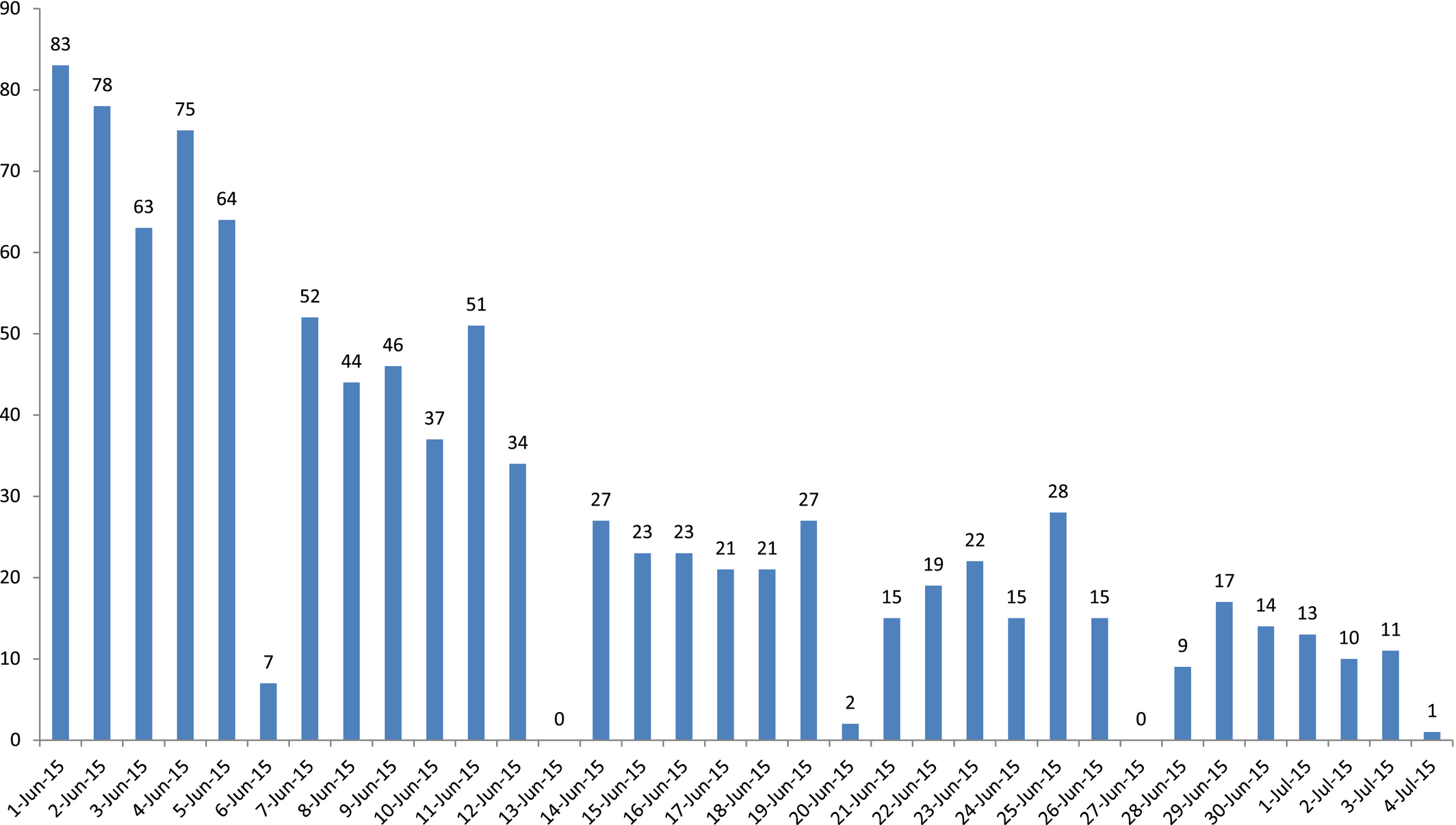
Total Daily Sales of the June 2015 Issue of Menta® [Color figure can be viewed at wileyonlinelibrary.com]

After examining the sales profile of the individual retailers and consulting Yedioth's experts, we made the assumption that all retailers have the same the sales profile, and that for a given issue, a retailer's daily sales profile is the same as the aggregate daily sales profile. This assumption is reasonable since all the retailers in the field study belong to the same supermarket chain.

We used the data from the EDI system to obtain an estimate of the daily sales distribution in each month. First, we neutralized the effect of the weekend by ignoring the observations from Thursdays and Saturdays, and fit a logarithmic decaying curve to the remaining data. This was done for three different issues (June 2015, R ² = 0.96; July 2015, R ² = 0.85; and August 2015, R ² = 0.91). Next, for the same issues, we obtained the Thursday and Saturday coefficients by calculating the ratio of the real daily sales to the predicted daily sales without the weekend effect. The coefficients of the other days of the week were set to one. We multiplied the daily sales predicted by the logarithmic curve, by the coefficients (shifted to match the varying days of the week in each issue), and normalized the total monthly sales to one, to obtain estimates for the proportions of the daily sales in future months. We also accounted for the varying number of days on the shelf of different issues. For each issue, we relied on different fitted curves and coefficients, depending on the available data at the time of decision. Table 4 provides a summary of information used in the field study while Figure 8 summarizes the order of actions in a typical month.

Table 4

Summary of Information Used in the Field Study

Month	July	August	October	November	December
Our policy followed	–	√	–	–	√
Uncensoring used	–	–	√	√	√
Months to calculate	June	June	June (30%),	July (60%),	July (50%),
daily sales distribution			July (70%)	August (40%)	August (50%)

Figure 8

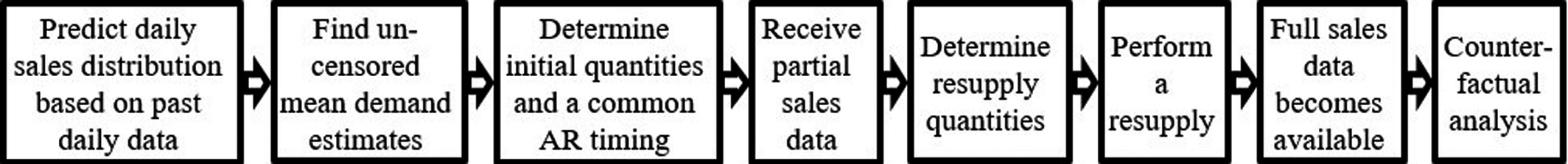
Actions Taken in a Typical Month

For the pilot field study, we relied on Yedioth's experts’ analysis as to the lack of demand correlation over time, but after the completion of the pilot we used the full EDI data to test this. We calculated the correlation coefficient based on a total of 870 pairs of observations. Each pair consisted of (uncensored) demand before and after the AR in each month of implementation. The resulting coefficient is ρ = 0.271, which implies a positive but weak correlation between sales over time. The significance of the correlation is p _v < 0.001 based on a standard t‐test (see Appendix C for details). This implies that Yedioth can draw little or no insight from demand forecast updating.

Although the ultimate aim was to perform a second printing for Menta® based on the suggestions of our model, during the pilot field study, a convenient and readily available source of magazines for the additional replenishment was a central excess stock of Menta® magazines, which Yedioth prints and keeps to hedge against uncertain yields (a common practice in the print industry). This option required almost no logistical modifications while enabling us to convince Yedioth's decision makers about the importance of our proposed model. There was always enough excess stock to accomplish the replenishment.

The unit cost information was obtained as follows. The unit selling price is known (V = 21.2 NIS). The unit production cost was obtained from the production department (c = 2.54 NIS) and is the same for both production runs. The unit disposal cost, also obtained from Yedioth, was estimated as h = −1 NIS. This cost is negative due to a secondary use of the returned copies (selling to secondary markets at a reduced price, using as samples in selling subscriptions, handing out to visitors, etc.). The unit penalty cost, estimated by the marketing department as p = 2 NIS, incorporates the loss of potential readers and the loss of exposure to advertisement. This means a high critical ratio of 0.93. To avoid the fixed visit cost, we asked the sales agents to perform their standard additional visit at the timing suggested by our model.

During the pilot field study we encountered and addressed several challenges.

Lag in obtaining the EDI data. This lag was generally around 48 hours, which meant that our decisions regarding the additional shipment quantities were based on slightly less information than desired. Nevertheless, we increased Yedioth's profits, and expect even better results when this lag is eliminated.

Lack of timely information regarding the number of days an issue will be on the shelves. Due to last‐minute changes common in the print industry, we had to make appropriate assumptions. The assumed number of days later turned out to deviate from the actual number of days by no more than two. Recalling the decline in the sales throughout the month, we believe that this mismatch had very little impact.

Decline in sales over the past years. As with many other print products around the world, Menta® is experiencing an overall decline in sales. The decaying sales pattern meant that some historical data did not predict future demand. After consulting Yedioth's experts, only relevant observations were used in estimating the mean demands. It should be pointed out, however, that not all the 174 retailers that participated in the study experienced decaying sales. Some showed no trend, and a minority even showed an increase over the past years.

Censored demand, as detailed in Appendix A. We addressed this issue by implementing the uncensoring procedure described earlier in this section, which did not change estimates much.

Skepticism of the RD. We compared the initial quantities obtained from our two‐phase model to those obtained by Yedioth's RD for each retailer. The company's quantities were often lower than the quantities we suggested. This is possibly because the in‐house model did not consider properly the penalty cost and the revenue loss from a lost sales. We discussed the quantities with Yedioth each time a large difference occurred. While Yedioth's RD partly accepted our suggestions, it did make minor manual adjustments to them. Nonetheless, our model managed to perform better than Yedioth's RD even after these adjustments. As we demonstrate later, our model without adjustments would have performed even better. Moreover, we compared the quantities suggested by our model to NV quantities.

Lack of cooperation on the part of the sales agents and the retailers. Due to the magnitude of demand, the quantities to be supplied during the additional visit were sometimes as low as a single copy. Additionally, our model can sometimes suggest performing an additional visit when the on‐hand stock level is positive. Due to various objections from the sales agents, we surrendered the idea of one‐copy replenishing for a retailer who had positive on‐hand stock. Our model outperformed Yedioth's model even with these changes.

Table 5 contains the PRUC for the system of 174 retailers for each of the five months under consideration. The profits in Equation (11) are aggregated over the 174 retailers. The results point to a significant savings provided by our model. On average, 19.35% of the gap between a system of separate NVs and a system with perfect demand information can be overcome with the aid of our model, which is considered a particularly high savings for the print industry. Table 5 also reports the PRUC when we relax the constraint that the AR day to be the same for all retailers. For each month, we observe a minor increase ( < 1% in all cases) in the PRUC. We note that the optimal unconstrained AR days are scattered around the optimal constrained AR day. More importantly, we emphasize that this unconstrained solution information is presented for illustrative purposes as this policy is not implementable. Logistical constraints dictate that geographically close retailers have the same AR day.

Table 5

PRUC, Second Half of 2015

	July	August	October	November	December
PRUC, joint AR day	19.58%	22.50%	19.08%	17.77%	17.81%
PRUC, different AR days	20.36%	23.18%	19.99%	18.69%	18.66%

We performed a counterfactual analysis³ to compare the performance of the various models. In August and December, Yedioth followed our proposed policy. In the other months, they followed their own policy. Upon obtaining complete sales data, the policies were compared. Thus, for July, October and November, the analysis of Yedioth's policy is real while the analysis of our policy is counterfactual. For August and December, the opposite is true. For each month, we also examined what would have happened had the standard NV model or Avrahami et al. (2014)'s model been followed. We remind the reader that the essence of Avrahami et al. (2014)'s model is that the second supply comes from pooled undistributed stock held back at an exogenously determined time, as opposed to our model which allows for a second production at an endogenously determined time. Since manual adjustments to our suggested decisions were applied by Yedioth, for August and December we also provide a counterfactual analysis of what would have happened if our model had been used as is.

To evaluate the difference in the models’ performance, we needed to estimate the lost sales at retailers with a stockout. The number of lost sales was estimated using the EDI data to determine when the last copy was sold. We then approximated the lost sales to be the expected demand until the end of the period.

Table 6 presents the comparison (see Table 7 for the results of statistical tests), with headers indicating which model was used. Note that the actual sales, quantity produced, returns, and lost sales in July, October and November appear in the second column, while the actual numbers in August and December appear in the fifth column. These numbers are in bold for easy reference. Our model tended to suggest that an additional visit should be carried out on average after 55% of the monthly predicted demand has been observed.

Table 6

Counterfactual Analysis, Second Half of 2015

	Yedioth's policy	NV	Avrahami	Two‐phase adjusted	Two‐phase
July
Sales	518	571	572	–	577
Quantity produced	713	910	876	–	890
Returns	195	339	304	–	313
Lost sales	71	18	17	–	12
Total profit	9,223.58	10,096.8	10,171.36	–	10,260.8
August
Sales	390	440	438	422	439
Quantity produced	599	943	909	881	893
Returns	209	503	471	459	454
Lost sales	65	15	17	33	16
Total profit	6,825.54	7,405.78	7,413.74	7,101.66	7,460.58
October
Sales	369	459	450	–	462
Quantity produced	533	937	801	–	849
Returns	164	478	369	–	387
Lost sales	107	17	26	–	14
Total profit	6,418.98	7,794.82	7,822.46	–	7,996.94
November
Sales	534	560	572	–	577
Quantity produced	732	824	886	–	834
Returns	198	264	314	–	257
Lost sales	91	65	53	–	48
Total profit	9,477.52	9,913.04	10,083.96	–	10,275.04
December
Sales	441	462	461	463	465
Quantity produced	661	812	791	727	739
Returns	220	350	330	264	285
Lost sales	46	25	26	24	22
Total profit	7,798.26	8,031.92	8,042.06	8,185.02	8,221.94

Table 7

Pairwise Comparison of Policies (percentage)

	July	August	October	November	December
Two‐Phase Adjusted vs. Yedioth's	–	4.0%	–	–	5.0%
Two‐Phase Adjusted vs. NV	–	−4.1%	–	–	1.9%
NV vs. Yedioth's^*	9.5%	8.5%^⋆	21.4%	4.6%	3.0%
Two‐Phase vs. Yedioth's^*+	11.2%^⋆	9.3%	24.6%^⋆	8.4%^⋆	5.4%
Two‐Phase vs. NV^*+	1.6%^⋆	0.7%^⋆	2.6%^⋆	3.7%^⋆	2.4%^⋆
Two‐Phase vs. Two‐Phase Adjusted⁺	–	5.1%^⋆	–	–	0.5%
Avrahami et al. (2014) vs. Yedioth's^*	10.3%^⋆	8.6%	21.9%	6.4%	3.1%
Avrahami et al. (2014) vs. NV^*	0.7%^⋆	0.1%	0.4%^⋆	1.7%	0.1%
Two‐Phase Adjusted vs. Avrahami et al. (2014)	–	−4.2%	–	–	1.8%
Two‐Phase vs. Avrahami et al. (2014)^*+	0.9%	0.6%^⋆	2.2%	1.9%^⋆	2.2%^⋆

One can observe that our two‐phase model, even when manually adjusted, always gives better results than Yedioth's model. While increasing the total production quantity and the number of returns, it also reduces the number of lost sales (which is the same as increasing the number of sales). In November, the demand in the first phase happened to be larger than the mean demand, and our model compensated for that by suggesting producing more in the second phase, such that the total quantity produced exceeded the one in the NV model. Compared to the standard NV model and Avrahami et al. (2014)'s model, our two‐phase adjusted model is superior in four out of five months. Moreover, in all five months, the two‐phase model without adjustments is superior to all others. While a considerable portion of the improvement over Yedioth's policy can be achieved by simply implementing a standard NV model, our two‐phase model can increase profits further. The reason is that the two‐phase model with an optimally timed additional visit captures the benefits of risk pooling over time and enables the use of in‐cycle sales information. We attribute the reduced difference between Two‐Phase and Two‐Phase Adjusted in December compared to August to the trust that we built with Yedioth which meant that they were less likely to “adjust.”

Table 7 details the pairwise percentage increase in the profit (relative to the latter policy in each pair) for each month. As expected, Yedioth gave the lowest profit followed by NV, Avrahami et al. (2014), and Two‐Phase, which gave the highest profit. Moreover, Two‐Phase gave higher profit than Two‐Phase Adjusted. We verified the significance of these differences through a series of one‐tailed Wilcoxon signed‐rank tests at the 5% significance level. We used this non‐parametric test rather than a paired t‐test because our data was not normally distributed. The stars in the first column indicate that the result is significant for the overall profit across the five months of implementation. The stars in the other columns indicate that the result is significant for the individual retailer profit for the month indicated. The plus signs in the first column indicate that the result is significant for the individual retailer profit for all the months for which data was available. Based on these last tests our policy (Two‐Phase) performs significantly better than all the other policies.

Expanded Implementation at Yedioth

After the successful completion of the pilot field study, Yedioth's management was ready to fully implement the proposed two‐phase model and change the way they make lotsizing decisions. In fact, Yedioth scaled our model to all its printed magazine titles and started routinely following it. Initial shipment quantities are determined accounting for the additional distribution later in the sales period. For simplicity, Yedioth decided to determine these quantities based on a heuristic whereby a NV problem is solved for the first phase alone, and the resupply quantities are determined by our algorithm. Since multiple magazine titles are involved, Yedioth examines several practical options for the AR day and selects the best one subject to the availability of the salesperson. Given that most Yedioth magazines are weekly (in fact, only Menta® is monthly), there are only a few options for the AR day. Moreover, Yedioth resolved the issue that had caused the lag in obtaining the EDI data.

Contrary to Yedioth's initial willingness to engage in another printing run in the case of a successful pilot, the company eventually decided not to perform a second printing. Rather, it continues to use the additional copies that are printed as safety stock against uncertain yield. Yedioth's experts estimate the savings from the changes to be 250,000 USD per year, net of the logistics cost.

Concluding Remarks

In this work, we presented a model and solution that we implemented at a major media group in Israel, Yedioth. We observed a considerable increase in profits compared to the existing policy. Our model is also shown to be superior to the standard NV model and Avrahami et al. (2014)'s model. Recalling that Yedioth has as many as 8000 points‐of‐sale, the increase in profits due to our two‐phase model is substantial. Moreover, Yedioth now successfully follows our two‐phase model for all their printed magazines, thus achieving a competitive advantage through a considerable cost saving, even if logistics costs, which do not exceed 2% in the case of Yedioth, are taken into account. The implementation at Yedioth shows robustness of our model. The savings from our model which assumes Poisson demand are considerable, even if demand may not be Poisson.

We analyzed a two‐phase NV problem with a possibility for an AR and replenishment. The novelty of our approach is in simultaneously determining the optimal initial order quantity, the optimal AR timing and the optimal order‐up‐to level at the time of the AR. We identify the problem's structural properties and propose an exact and tractable solution algorithm. The algorithm scans

O (S^{*} (0))

different intervals. For each interval, we scan

O (S_{0}^{*})

initial quantities. In this way, Newton's search is employed

O (S^{*} (0) \cdot S_{0}^{*})

times. From our computational experiments, we observed that due to our elimination criteria, the number of Newton searches is far less than this upper bound. Although

S^{*} (0)

and

S_{0}^{*}

can be large, for practical problems, the proposed algorithm requires a reasonable computational effort.

We also developed and tested a simple heuristic solution that works exceedingly well. Nonetheless, we prefer the slightly more involved optimal algorithm due to the substantial costs being considered. As retail costs are significant in the total value chain of a product, the savings enabled by our model are important for decision makers. Our model is general enough to be applied to other printing houses and industries that have similar setup conditions and operate within the NV framework. This includes bakeries (some of which routinely practice double‐baking with the second batch being based on observed demand), other food industries, and the apparel industry.

A possible direction for future developments is to consider demand forecast update at the time of the AR, which would enable decision makers to obtain improved insights. In the case of Yedioth, however, this is not crucial as demand exhibits very low correlation over time.

Footnotes

Acknowledgment

The authors express their gratitude to Yedioth Group for providing the necessary data and running the pilot field study.

After our cooperation ended, Yedioth decided to implement our methodology without a second production run (see section ) but the constraint on a single AR day remained.

The weekend in Israel is on Friday and Saturday, and on Saturdays most shops are closed.

Ideally, we would have randomly picked a subset of retailers to follow our proposed policy while leaving the others to perform the current policy. Such an experiment was not allowed by Yedioth.

ORCID

Dina Smirnov

Yale T. Herer

References

Avrahami

Herer

Y. T.

Levi

. 2014. Matching supply and demand: delayed two‐phase distribution at Yedioth group‐models, algorithms, and information technology. Interfaces 44(5): 445–460.

Bulinskaya

1964. Some results concerning optimum inventory policies. Theory Prob. Appl. 9(3): 389–403.

Cachon

G. P.

Swinney

. 2009. Purchasing, pricing, and quick response in the presence of strategic consumers. Management Sci. 55(3): 497–511.

Cachon

G. P.

Swinney

. 2011. The value of fast fashion: Quick response, enhanced design, and strategic consumer behavior. Management Sci. 57(4): 778–795.

Choi

T. M.

Yan

. 2003. Optimal two‐stage ordering policy with Bayesian information updating. J. Oper. Res. Soc. 54(8): 846–859.

Conrad

S. A.

1976. Sales data and the estimation of demand. Oper. Res. Quart. 27(1i): 123–127.

Crowston

W. B.

Hausman

W. H.

Kampe

W. R.

II . 1973. Multistage production for stochastic seasonal demand. Management Sci. 19(8): 924–935.

Donohue

K. L.

2000. Efficient supply contracts for fashion goods with forecast updating and two production modes. Management Sci. 46(11): 1397–1411.

Eppen

G. D.

Iyer

A. V.

. 1997. Improved fashion buying with Bayesian updates. Oper. Res. 45(6): 805–819.

10.

Erkip

N. K.

1984. A restricted class of allocation policies in a two‐echelon inventory system. Technical Report 628, School of Operations Research and Industrial Engineering, Cornell University, Ithaca, New York.

11.

Fisher

Raman

. 1996. Reducing the cost of demand uncertainty through accurate response to early sales. Oper. Res. 44(1): 87–99.

12.

van derHeijden

M. C.

1999. Multi‐echelon inventory control in divergent systems with shipping frequencies. Eur. J. Oper. Res. 116(2): 331–351.

13.

Jönsson

Silver

. 1987. Analysis of a two‐echelon inventory control system with complete redistribution. Management Sci. 33(2): 215–227.

14.

Linh

C. T.

Hong

. 2009. Channel coordination through a revenue sharing contract in a two‐period newsboy problem. Eur. J. Oper. Res. 198(3): 822–829.

15.

Liu

Song

. 2012. Good and bad news about the (s; t) policy. Manufact. Serv. Oper. Manag. 14(1): 42–49.

16.

McGavin

E. J.

Schwarz

L. B.

Ward

J. E.

. 1993. Two‐interval inventory allocation policies in a one‐warehouse n‐identical‐retailer distribution system. Management Sci. 39(9): 1092–1107.

17.

Milner

J. M.

Kouvelis

. 2005. Order quantity and timing flexibility in supply chains: The role of demand characteristics. Management Sci. 51(6): 970–985.

18.

Murray

G. R.

Jr. Silver

E. A.

. 1966. A Bayesian analysis of the style goods inventory problem. Management Sci. 12(11): 785–797.

19.

Nambiar

Simchi‐Levi

Wang

. 2020. Dynamic inventory allocation with demand learning for seasonal goods. Prod. Oper. Manag. 30(3): 750–765.

20.

Rao

U. S.

2003. Properties of the periodic review (r; t) inventory control policy for stationary, stochastic demand. Manufact. Serv. Oper. Manag. 5(1): 37–53.

21.

Shang

K. H.

Tao

Zhou

S. X.

. (2015). Optimizing reorder intervals for two‐echelon distribution systems with stochastic demand. Oper. Res. 63(2): 458–475.

22.

Smirnov

Avrahami

Herer

Y. T.

. 2021. The multi‐period delayed distribution problem. Working Paper, Technion–Israel Institute of Technology.

23.

Wang

2013. A periodic‐review inventory control policy for a two‐level supply chain with multiple retailers and stochastic demand. Eur. J. Oper. Res. 230(1): 53–62.

24.

Wang

Axsäter

. 2013. Fixed‐interval joint‐replenishment policies for distribution systems with multiple retailers and stochastic demand. Nav. Res. Logist. 60(8): 637–651.

25.

Wang

Tomlin

. 2009. To wait or not to wait: Optimal ordering under lead time uncertainty and forecast updating. Nav. Res. Logist. 56(8): 766–779.

Two‐Phase Newsvendor with Optimally Timed Additional Replenishment: Model,Algorithm,Case Study

Abstract

Keywords

Introduction

Literature Review

Problem Statement

Planning Horizon and Demand Process

Order of Events and Cost Structure

Analysis

Objective Function

Breakpoints

Bounds on the Initial Order Quantity, Q 0 *

Analysis with Respect to the Additional Review Timing

Solution Algorithm

Discrete‐Time Heuristic

Computational Experiments

Implementation at Yedioth Group

Adapting the Model to Yedioth's Case

Pilot Study Details and Results

Expanded Implementation at Yedioth

Concluding Remarks

Footnotes

Acknowledgment

ORCID

References

Bounds on the Initial Order Quantity,
$Q_{0}^{*}$