
Abstract
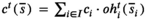
Inventory optimization approaches typically optimize steady‐state performance, but do not consider the transition of an initial state to the optimized state. In this study, we address this transition. Our research is motivated by a company that implemented an improved inventory policy for its spare parts division. The improved policy suggested new base stock levels for the majority of the parts. For parts with increased base stock levels, inventory increases were realized after the part lead times, but for low‐demand parts with decreased base stock levels, inventory reductions were slow. As a result, inventory cost increased over the first months after the new inventory policy had been introduced and exceeded the inventory budget substantially. To avoid such undesirable effects, base stock level changes must be phased in. We consider a multi‐item spare parts inventory system, initially operating under an item approach inventory policy that achieves identical fill rates for all parts. Our approach addresses the transition to a superior system approach inventory policy that maximizes the system fill rate. We model the inventory transition as a finite‐horizon optimization problem and apply column generation and a marginal analysis heuristic to determine transient base stock levels for all parts. Using data from the company that motivated our research, we illustrate how the transition can be controlled to quickly improve fill rates without exceeding the initial inventory budget.
Introduction
The trigger of inventory optimization projects is often a suboptimal performance of the current inventory system. In spare parts management, for instance, companies can set base stock levels such that a certain fill rate is achieved by every individual part. This approach is referred to as
Implementing a system approach requires the adjustment of inventory control policy parameters. For example, base stock levels of inexpensive fast movers are increased and base stock levels of expensive slow movers are reduced. Overall inventory performance is improved once the inventory system has reached its new steady state. However, during the transition to the new steady state, system fill rate or system inventory holding cost can deteriorate temporarily, particularly if lead times are long or demand rates are low.
We experienced this in an inventory optimization project with the service division of a global business‐to‐business (B2B) equipment manufacturer. The company generates annual multi‐billion euros turnover and operates in more than 50 countries. Its service division offers repair and maintenance services for the specialized and expensive equipment. The division wanted to improve its inventory performance but the inventory budget was restricted and we were asked to improve the system fill rate without exceeding the current budget. We suggested moving the inventory system from an item approach to a system approach and projected a long‐run system fill rate increase of 12 percentage points while keeping the inventory holding cost constant. After pilot implementation of the new approach, the system fill rate started to improve, but the inventory holding cost increased by more than 20% within four months (Figure 1). This placed a major burden on the service organization's inventory budget and it took more than a year for the inventory holding cost to finally reach the projected value.
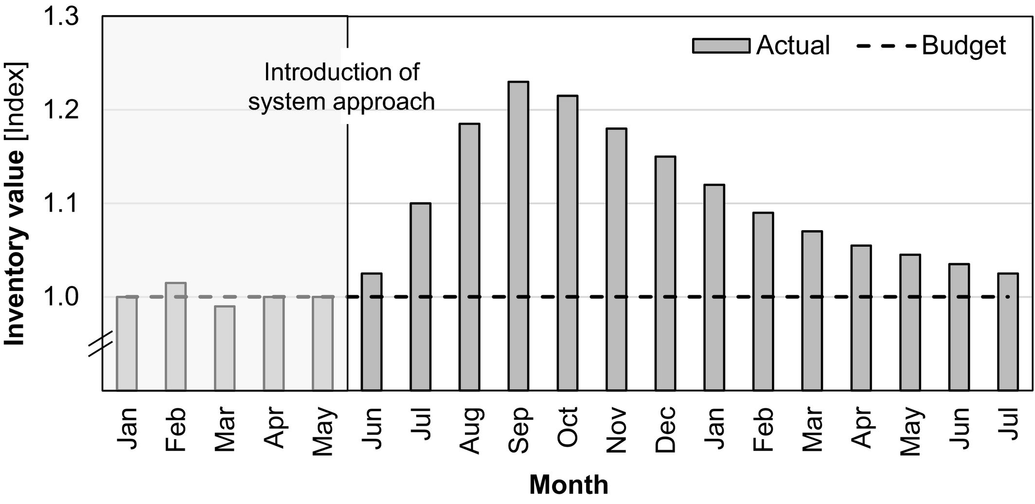
Inventory Index Development at the Service Division after Introducing the System Approach Base Stock Levels in May
The observed increase in inventory cost is a severe issue, since complying with inventory budgets is of critical importance to companies. Companies establish inventory budgets because the capital they can invest in inventory is restricted (Silver et al. 2016, Yang et al. 2017). Requiring significantly more capital, even if only temporarily, can cause severe financial straits and even impacts the company's valuation. Moreover, the negative consequences of increased inventory cost during the transition period are not limited to the direct financial impact. Major changes in inventory policies like moving from an item approach to a system approach are usually initiated in the scope of large and costly inventory projects. If the inventory performance falls short of its targets and expectations, the pressure on accountable divisions can be substantial.
These observations motivated our research on controlling the transition of inventory systems when the inventory policy changes. We analyze the transient behavior of a spare parts inventory system that operates under a periodic review base stock policy. The goal of our approach is to phase‐in changes in base stock levels over time while keeping inventory holding cost within a given budget during the transition.
We focus on analyzing the base stock level transition of an inventory system that moves from an item approach to a system approach, taking into account replenishment lead times and expected future demands. However, our model is not restricted to managing transitions of inventory systems starting from an item approach. It can be generally applied to arbitrary inventory systems that operate under periodic review base stock policies and that require an adaption of the base stock levels to a system approach. Such adaptions might be triggered, for example, if lead times or prices are renegotiated with suppliers, new suppliers are introduced, new customers are acquired, or major customers terminate their service contracts (Çetinkaya and Parlar 2010).
We contribute to the inventory control literature by considering the transition of a multi‐item inventory system from a current state to an optimized state, which is a topic that has not previously been addressed. We formulate the problem as a multi‐period optimization problem and present two solution approaches that rely on column generation and on marginal analysis, respectively. For small and moderate size problems, for which we can determine upper bounds on the objective function values, both approaches generate solutions that are close to optimal. Large size problems can only be solved by marginal analysis and we use the approach in an extended case study that is based on data from a global equipment manufacturer.
This study is structured as follows. In section 2, we review the literature. In section 3, we present a model for optimizing the inventory system transition. In section 4, we introduce two solution approaches. In section 5, we present numerical results based on data from the service division of the global manufacturer that motivated our research. In section 6, we summarize our findings and conclude.
Literature Review
We review steady‐state system approaches with modeling assumptions similar to our work, and non‐steady‐state inventory models for base stock level transitions. We also review two relevant solution techniques for system approach optimization problems. For a comprehensive overview of the literature on spare parts inventory systems, we refer to Sherbrooke (2004), Muckstadt (2005), Basten and Van Houtum (2014), and Van Houtum and Kranenburg (2015).
System approaches for spare parts inventory systems have gained increasing attention since their introduction in the seminal paper by Sherbrooke (1968). Their benefits compared to simpler item approaches have been shown by Mitchell (1988), Thonemann et al. (2002), Rustenburg et al. (2003), and Sherbrooke (2004). Spare parts inventory systems that operate under a periodic review base stock policy have been analyzed by Mitchell (1988), Cohen et al. (1989), and Cohen et al. (1992). Budget‐constrained, service maximizing system approaches have been analyzed by Rustenburg et al. (2000, 2003) and Sherbrooke (2004). Schwarz et al. (1985) maximize the system fill rate subject to a constraint on the system safety stock.
While most system approach models consider the initial supply of spare parts, there are only a few models that include the current state of a running inventory system. For such a system, Rustenburg et al. (2000) address a budget‐constrained re‐supply problem. They assume annual budgets for the total purchasing cost of new parts, which arrive after a fixed lead time. They develop operational re‐supply strategies for spending the limited budget, but do not cover situations in which the optimal target base stock levels change.
Van Houtum and Kranenburg (2015 ch. 2.8) introduce a modified system approach for periodic base stock level optimization. They account for the current inventory position of each spare part by modifying the cost function of the standard initial supply model when updating the base stock levels. While their approach generates good solutions for the next planning period, it is myopic and does not aim to reach the standard system approach base stock levels. This is reasonable for inventory systems that already operate under a system approach, when changes in base stock levels are typically minor. Their approach also assumes steady‐state behavior of the system in each period with quickly realized changes in the base stock levels. The authors note that it is necessary to consider the transient behavior of the inventory system if their assumptions do not hold, for example, if parts have long replenishment lead times. We address such situations with our research.
Several publications address the non‐steady‐state transition period when steady‐state base stock levels change for single items. When base stock levels increase, the implication in a single‐item setting is straightforward: new parts must be ordered and arrive after the replenishment lead time. When base stock levels decrease, inventory above the reduced base stock level must be considered. Pinçe and Dekker (2011) note that in such situations “timely adaption of the base stock levels is crucial for optimal stock control” (p. 83). They adapt the steady‐state base stock policy for a single, low demand item with a fixed lead time and decreasing demand and propose a transition control policy that minimizes the total expected cost during the transition. Similar to our model, their policy is based on the current inventory position of the item, but it only allows for two different base stock levels and focuses on the timing of the switch. Our model allows for multiple adjustments in base stock levels during the transition period, which is hypothesized by Pinçe and Dekker (2011) to improve results. Teunter and Klein Haneveld (2002) develop an ordering policy for the end‐of‐life phase of service parts with stationary, Poisson‐distributed demand. Assuming a higher replenishment price and risk of obsolescence in the final phase, they propose a sequence of decreasing base stock levels for a deterministic planning horizon of a single item. Çetinkaya and Parlar (2010) consider the introduction of a periodic review base stock policy without an explicit spare parts focus. In their single‐item setting, the target inventory policy is similar to ours. However, the authors do not consider inventory systems with multiple items and do not include replenishment lead times. All of the reviewed non‐steady‐state models focus on the transition of a single item and are not directly applicable to the multi‐item problem that we consider.
We apply two solution approaches to solve our optimization problem. The first approach, decomposition and column generation, exploits structural properties of multi‐item spare parts systems. Instead of solving the original complex optimization problem, the problem is decomposed by spare part and the resulting single‐item optimization problems are solved repeatedly. This method has recently received increasing attention in the multi‐item spare parts inventory optimization literature (Alvarez et al. 2013, 2015, Arts 2017, Drent and Arts 2020, Kranenburg and Van Houtum 2007, Topan et al. 2010, Topan et al. 2017, Wong et al. 2007). Details on fundamentals and theoretical background of decomposition and column generation are provided by Dantzig and Wolfe (1960) and Desrosiers and Lübbecke (2005).
Our second solution approach, marginal analysis, is a well‐known solution technique for optimizing spare parts inventory systems that operate under a system approach (Sherbrooke 2004, Van Houtum and Kranenburg 2015). The general principle is to compare the cost of increasing a spare part's base stock level by one unit with its impact on the system's performance (e.g., the expected backorders or the system fill rate). In each iteration, the base stock level of the part with the highest performance improvement per monetary unit spent is increased. The procedure is repeated successively until the system target is reached. Marginal analysis is efficient, provides good results, and is easy to implement in practice. It has been applied to various spare parts inventory optimization problems, for example, by Wong et al. (2005, 2007) and Topan et al. (2017). For a finite‐horizon periodic review setting, Caggiano et al. (2006) apply heuristics that are based on marginal analysis to make operational repair and inventory allocation decisions. We use this solution approach to determine target base stock levels for multiple items and multiple periods based on the expected system state.
Problem Formulation and Mathematical Model
We consider a multi‐item spare parts inventory system that operates under a periodic review base stock policy (e.g., Cohen et al. 1992, Sherbrooke 2004). This inventory control policy is suited when spare parts are ordered periodically and is applied in many real‐world spare parts inventory systems (Cavalieri et al. 2008, Tiemessen et al. 2013, Wang 2012). It is also applied at the company that motivated our research. We denote the set of spare parts 


We will next discuss the model of the steady‐state inventory system and define the initial state of the inventory system under the item approach, as well as the target state of the inventory system under the system approach. Then, we will build on the steady‐state model to optimize the inventory transition from the item approach to the system approach.
The Inventory System in Steady State
We denote the base stock level of part 


The fill rate of part 
The Inventory System under the Item Approach
Consider an inventory system that is operated under the item approach. The base stock levels 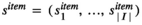

The Inventory System under the System Approach
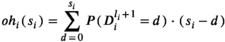
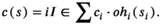
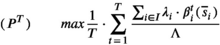
The base stock levels that maximize the system fill rate 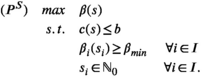


We solve problem (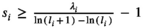
The Inventory Transition
The transition from the item approach to the system approach is realized during a finite planning horizon 


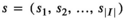
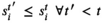
We model the transition as a sequence of base stock levels 


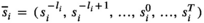


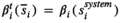
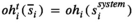
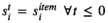
The base stock levels 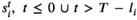


If 
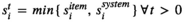
If 

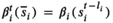
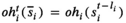
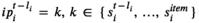
We can apply the steady‐state equations for increasing and constant base stock levels because of the characteristics of the base stock policy. Under the steady‐state base stock policy, the on‐hand inventory depends on the base stock level 


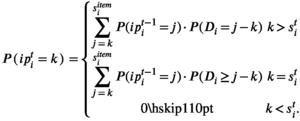
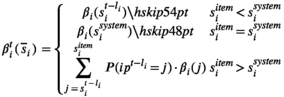
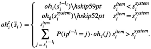
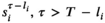
If 


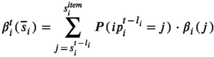
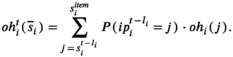
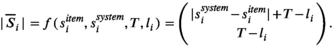
The transient fill rate and the transient on‐hand inventory at the end of period 


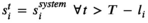
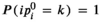
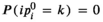
At the beginning of the transition, in period 0, the system is in steady‐state under the base stock policy with base stock levels 


(
Solution Approaches
We provide two solution approaches for problem (
Column Generation Approach
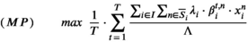
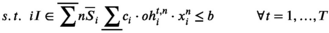
The optimization problem (
We first reformulate the problem (


For every part, the number of potential sequences 


In principle, it would be possible to determine 


To overcome this computational challenge, we relax the integrality constraints on 


We achieve this by solving the final (
Marginal Analysis Approach
Our second solution approach applies marginal analysis to all periods of the planning horizon. In every period, it considers the projected state of the inventory system, based on decisions of previous periods, different lead times of the parts, projected part demand, and restrictions on the base stock level sequences. We refer to this approach as marginal analysis approach (MA approach).
We perform a two‐stage algorithm on the planning horizon 


The 


The 


The detailed marginal analysis approach is provided in pseudocode in the Online Appendix.
We split the approach into two stages to mitigate the negative effects of its myopicness. The algorithm optimizes the base stock levels of the different periods successively. As a result, the transition to new base stock levels could be prolonged unnecessarily without the two stages. For parts with decreasing base stock levels, the myopicness of the approach could keep the base stock levels 


The two‐stage approach addresses this issue and ensures that base stock levels converge quickly to the target base stock levels, since it prioritizes the increase in base stock levels for parts with 


To guarantee the adherence to the budget constraint during the transition, only the first stage of the MA approach is crucial. Depending on the characteristics of the inventory system, the second stage can additionally increase the transient system fill rate during the transition, for example, if parts with increasing base stock levels have long lead times and parts with decreasing base stock levels have short lead times and high demands. For most inventory systems in the numerical study, however, the impact of the second stage is limited and most benefits are realized by applying the first stage.
The objective of the MA approach differs from the objective of the original problem (
Numerical Study
The numerical study presented in this section consists of two parts. First, we compare the performance of the CG approach and the MA approach for small to medium‐sized inventory systems with medium‐length planning horizons (section 5.1). Second, we analyze the value of optimizing the inventory transition in a case study based on company data (section 5.2). After applying the MA approach to a real‐world inventory system in section 5.2.1, we analyze the impact of changes in system characteristics in an extensive sensitivity analysis (section 5.2.2) and discuss managerial implications (section 5.2.3). We implemented all approaches in C++ and used Gurobi to solve the linear and integer programs. We conducted the computations on a Windows 10 64‐bit system with 16 GB memory and two Intel Xeon 2.30 GHz processors.
Performance Evaluation of the Solution Approaches
We benchmark the performance of the CG approach and the MA approach against the upper bound for small to medium‐sized inventory systems. The inventory systems are characterized by the number of parts, the initial system fill rate under the item approach, and the distributions of demand rates, unit holding costs, and lead times. Moreover, we vary the planning horizon of the transition. To obtain robust results, we randomly generate inventory systems with different parameter values. To get realistic scenarios, we base the parameter ranges on data from the company that motivated our research. Table 1 contains the parameter values that we cover in a full factorial analysis. We test the solution approaches for inventory systems with 20, 35, and 50 parts. Demand rates 


Parameter Values for the Performance Evaluation
We analyze four lead time settings. In the first setting, all parts have a lead time of 1 period. In the other settings, lead times are drawn from a discrete uniform distribution between 1 and an upper bound of 2, 3, and 4. We solve all instances with a minimum part fill rate of 50% and initial system fill rates of 75%, 85%, and 95%. The planning horizons are set to 10, 12, and 14 periods, which are reasonable time spans for the considered lead times. The combination of parameter values results in 35 × 4 = 972 settings. We randomly generate 20 instances per setting, leading to a total of 19440 instances. For all instances, we determine item approach and system approach base stock levels and then optimize the inventory transition with both solution approaches.
We assess the performance of the two approaches by evaluating the solutions and the runtimes for each instance. The solution quality is measured by comparing the objective value of the respective solution approach (


Table 2 summarizes the computational results for the 19440 tested instances. We report averages and maximum values for the gaps to the upper bound and runtimes with respect to the different parameter values (Table 2a–f) and present results across all instances at the end (Table 2g). The gaps to the upper bound are reported in percent. Across all instances (Table 2g), we observe that both solution approaches perform well with an average gap to the upper bound of 0.025% (CG approach) and 0.058% (MA approach). The maximum gaps of all 19440 instances are 0.644% and 1.163%, respectively. The gap of the CG approach to the upper bound is always smaller than or equal to the gap of the MA approach to the upper bound, as the base stock level sequences from the MA approach act as the starting solution for the CG approach. On average, the CG approach is able to close approximately half of the gap of the MA approach.
Summary of the Performance of the CG Approach and MA Approach
Analyzing the influence of different parameter values, we observe that the gap to the upper bound decreases with an increasing number of parts (Table 2a), thus with increasing problem size. This is particularly convenient since instances of real‐world size, like the ones we investigate in section 5.2, are large. The gaps also decrease with an increasing initial system fill rate 


While both solution approaches perform well with respect to gaps to the upper bound, the differences in runtimes are substantial. The MA approach provides a solution within milliseconds for all instances (maximum runtime of 13 milliseconds). The runtimes of the CG approach vary strongly. Across all instances, the average CG runtime is 45.92 seconds. However, the runtimes of single instances reveal large differences between 0.02 seconds (not explicitly shown in Table 2) and 26,122 seconds (7.25 hours). We observe this variation because the runtimes of the CG approach depend on the specific size of every instance, that is, the number of potential decision variables.
The problem size is driven by three elements: the number of parts in the system, the length of the planning horizon, and the difference between the item approach and the system approach base stock levels. The increase in average and maximum runtimes for the first two elements can be observed in Table 2a–f, respectively. An increasing number of parts and an increasing planning horizon result in longer runtimes. The third element, the difference in the base stock levels, drives the large spread of runtimes across all instances. It also drives the increasing runtimes for increasing demand parameters (Table 2c). In systems with low demand rates, more parts have minimum base stock levels of 1 under both the item approach and the system approach, thus fewer differences in the base stock levels and smaller problem sizes. Systems that transition from a lower system fill rate 


The results of the full factorial analysis demonstrate that applying column generation becomes impracticable for large inventory systems and long planning horizons. However, with the MA approach, we can obtain close‐to‐optimal solutions at short runtimes. To get further indications on how this performance might scale to larger inventory systems with longer planning horizons, we relax the full factorial setup. We fix the system parameters at the values for which we observed the maximum gaps of the MA approach to the upper bound (

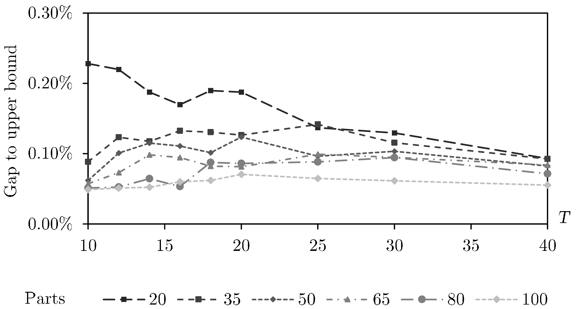
Average Gap of the MA Approach to the Upper Bound Depending on Planning Horizon and Number of Parts in the System
This further strengthens the positive indications for utilizing the MA approach for transitions that are impractical to solve with column generation. We will apply this solution approach to solve the real‐world inventory systems in the next section. Although we cannot provide upper bounds for the large systems, the results in this section suggest that we can expect the good performance of the MA approach also for larger planning problems.
The Value of Controlling the Transition
We benchmark the
Real‐World Application
We analyze the value of controlling the inventory transition based on data from the global manufacturer that motivated our research. The inventory system contains 3191 spare parts. Replenishment orders can be initiated on a daily basis (corresponding to a review period of one day) and arrive after lead times between 1 and 373 days. The demand rates vary between 0.5 and 1,524 units per year. The annual unit holding costs range between below 0.10 euros and above 30,000 euros per spare part, with an average of 416.80 euros.
Currently, the base stock levels of the system are determined with the item approach and the initial system fill rate is 85%. This results in annual system inventory holding cost of approximately 2.2 million euros. With a required minimum part fill rate of 50%, we predict an increase in the system fill rate of 13 percentage points with similar holding cost when moving the inventory system from an item approach to a system approach.
Figure 3 shows the development of the annual system inventory holding cost and the system fill rate for the uncontrolled and the controlled transition. We observe that directly implementing the system approach base stock levels (the uncontrolled transition) results in violations of the allowed holding cost budget of up to 15%, 100 days after the new base stock levels are introduced. On average, the budget is exceeded by 6.3% (142,000 euros) during the first year and by 1.8% (40,000 euros) during the second year of the transition.
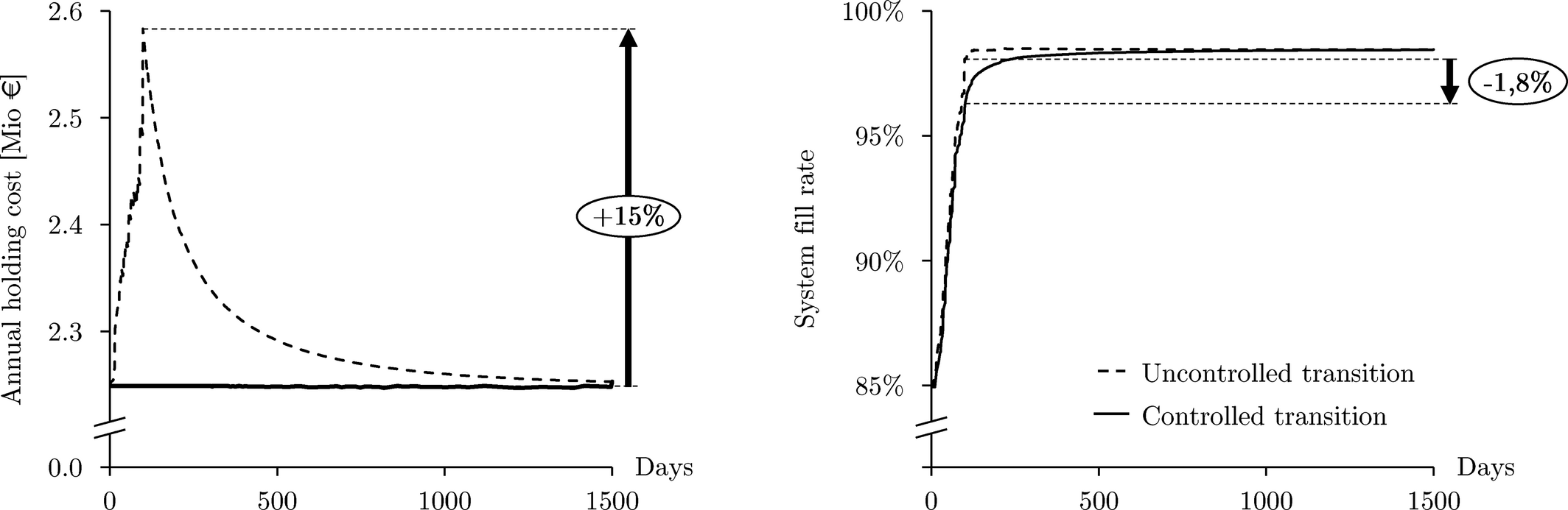
Comparison of the Controlled and the Uncontrolled Transition ‐ System Inventory Holding Cost (left) and System Fill Rate (right)
The controlled transition does not exceed the budget. The savings in holding cost go along with minor losses in the system fill rate of 0.7% on average during the first year and 0.1% during the second year, with a maximum of 1.8% on day 100. Those losses are the consequence of deliberately delaying the increase of base stock levels for certain parts to stay within the budget constraints in the controlled transition. This leads to a delayed increase in fill rates for the corresponding parts, and a lower system fill rate in the controlled transition than in the uncontrolled transition. However, the differences in system fill rate are marginal compared to the savings in system inventory holding cost. Similar to the uncontrolled transition, the system fill rate steeply increases at the beginning of the transition and the largest share of system fill rate improvement is realized quickly.
Figure 4 shows the base stock level transition and the resulting on‐hand inventory development for three exemplary parts. The first part (Part A) has a high demand over lead time, resulting in a higher system approach base stock level than under the item approach. Since it has relatively high unit holding cost, the increase of base stock levels is delayed and the system approach base stock level is reached relatively late in the transition. The changes in base stock levels are reflected in inventory after the lead time (90 days). Prolonging the base stock level increase of expensive parts is reasonable since all considered parts are of high criticality and any available part provides similar value to the company's B2B customers. Considering the benefit per monetary unit, it is therefore more beneficial to increase the base stock level of less expensive parts with a similar demand over lead time earlier. This can be observed for Part B. It has a similar demand over lead time but lower unit holding cost than Part A. Therefore, the base stock levels are increased earlier during the transition. The third part (Part C) has a rather low demand over lead time and relatively high unit holding cost. This results in a lower system approach base stock level than under the item approach. The system approach base stock level is set directly in period 1, however, it takes time until the projected steady‐state on‐hand inventory value is reached.
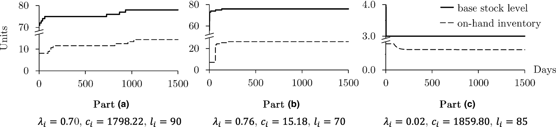
Transition of Base Stock Levels and Expected On‐Hand Inventories for Three Exemplary Parts
Sensitivity Analysis
In the real‐world application analyzed in the previous section, we observe significant savings in system inventory holding cost and only marginal losses in system fill rate when controlling the transition. In this section, we investigate how the characteristics of the inventory system (demand rates, unit holding costs, lead times, and initial system fill rates under the item approach) influence the impact on system holding cost and system fill rate during the transition.
We must find appropriate representations of the real‐world inventory system's characteristics that can be varied subsequently. Therefore, we describe the inventory system by the distributions of demand rates, unit holding costs, and lead times. We fitted various distributions to the parameter value realizations and found that the demand rates and the unit holding costs for different spare parts are well represented by lognormal distributions (

We substitute the original values for the part characteristics with the theoretical values obtained from the distributions. For every part in the original dataset, we first determine the percentile ranks of its demand rate 


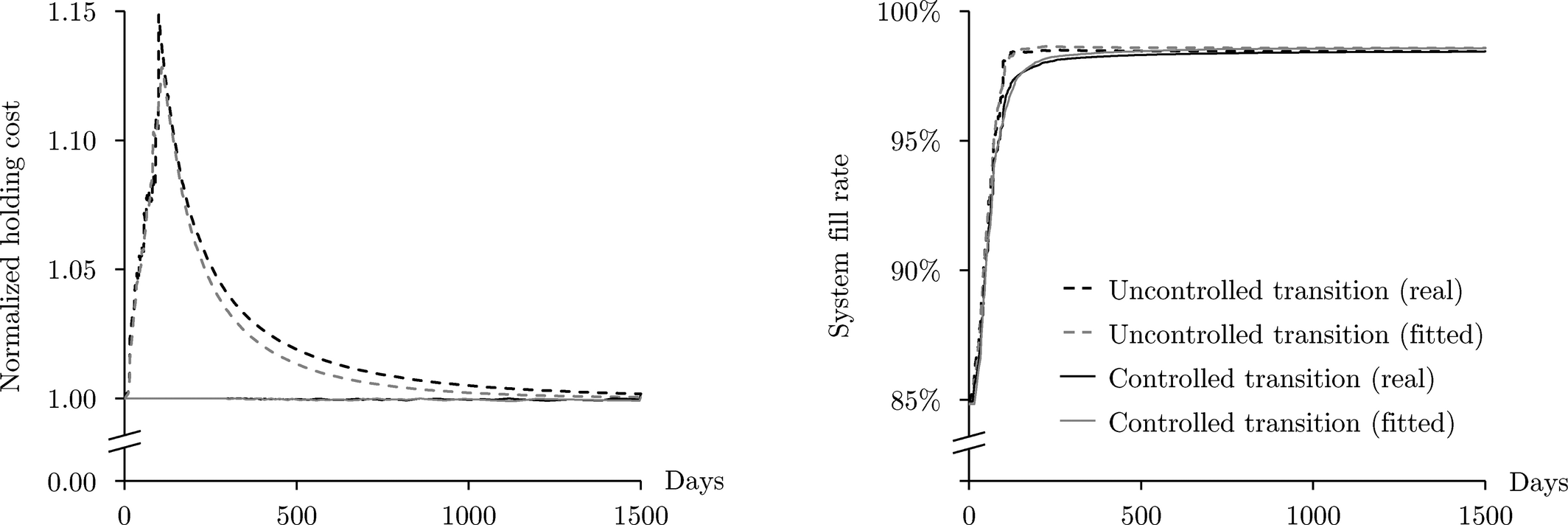
Comparison of the Transitions of the Real and the Fitted Inventory System ‐ System Inventory Holding Cost (left) and System Fill Rate (right)
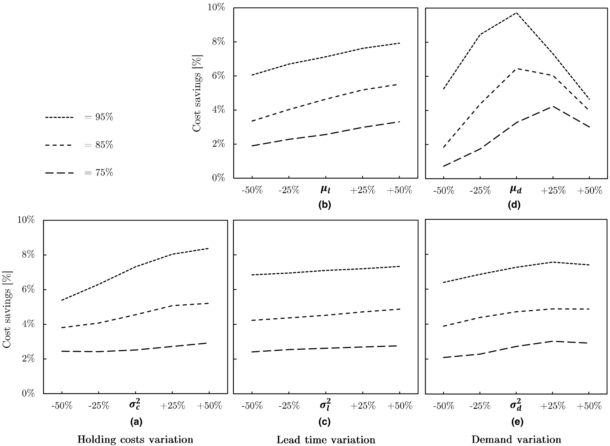
To analyze in which settings controlling the inventory transition is particularly beneficial, we vary the characteristics of the inventory system by modifying the corresponding distribution parameters. For the demand rates of the system's spare parts, we increase and decrease 


We analyze the transition for all different parameter combinations. Figures 6a–e show the aggregated effect of the different parameter values on the savings in system inventory holding cost during the first year of the controlled transition, compared to the uncontrolled transition. Across all systems, we observe the highest savings in system inventory holding cost for systems with high initial system fill rates 

Average Savings in System Inventory Holding Cost When Controlling the Transition Depending on the Inventory System Characteristics
The distribution of lead times also affects the cost savings. Longer lead times (Figure 6b) positively correlate with the savings due to their influence on the demand over lead time, which is the main driver for base stock levels. A higher demand over lead time yields higher initial base stock levels, and therefore more budget flexibility. The variance of the lead times (Figure 6c) has only little effect on the cost savings. We observe a weak positive influence of a higher spread in lead times, which is mainly driven by the long lead time for some parts and the truncation of the lead time distribution at 1.
The impact of demand parameters on the cost savings is ambiguous. Figure 6d shows the influence of the demand parameter 

We next analyze the impact of the inventory system characteristics on the relative difference in average system fill rate between the controlled and uncontrolled transition during the first year (Figure 7a–e). Across all system parameter values, the differences in average system fill rate are small and rarely exceed 1.5%. This underlines the value of controlling the inventory transition since it allows to save a significant amount of money while not significantly affecting the system fill rate. We also observe that the higher the initial system fill rate 

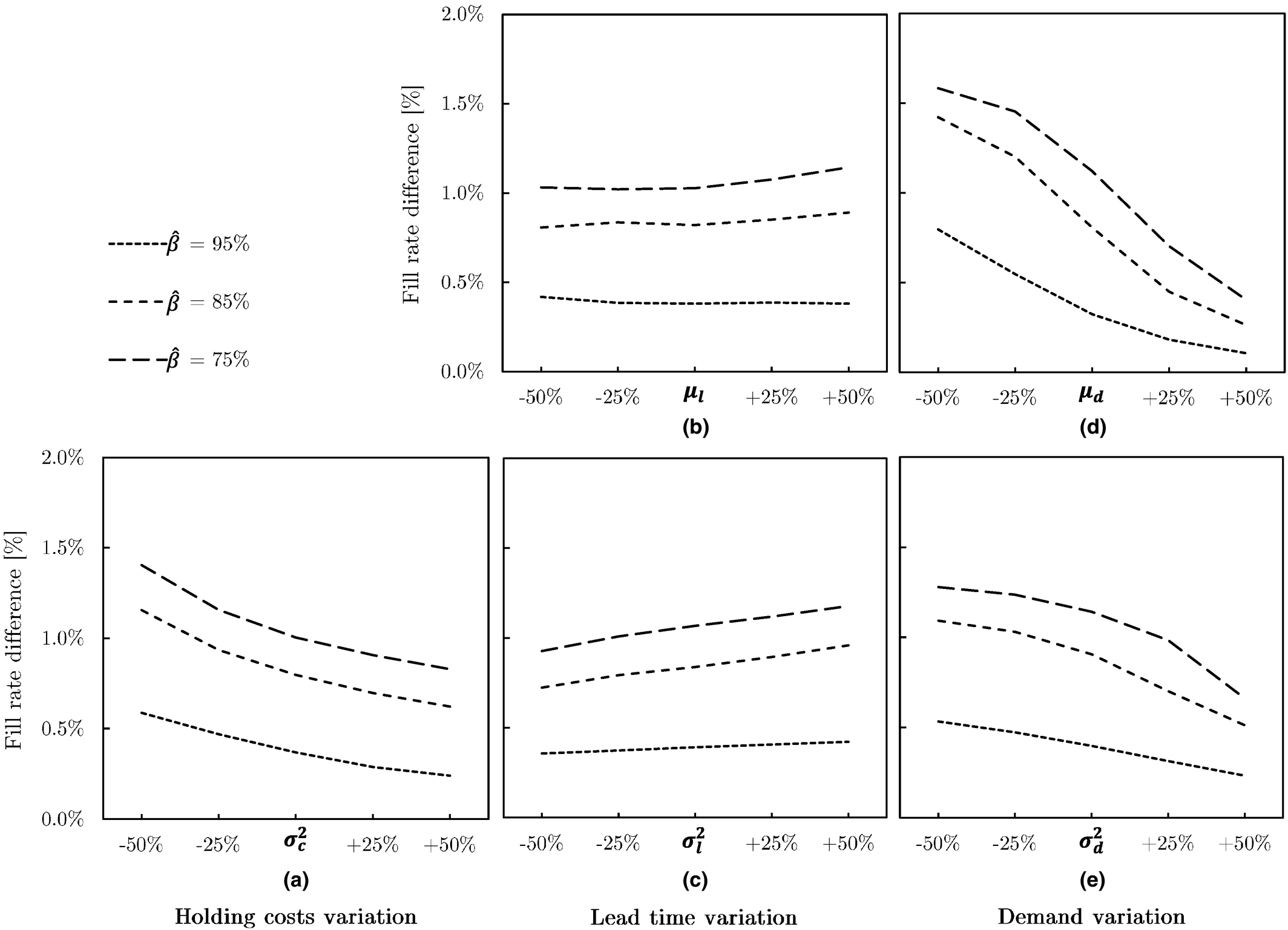
Relative Differences in Average System Fill Rate When Controlling the Transition Depending on the Inventory System Characteristics
The maximum periodic cost savings and the maximum fill rate difference during the transition show similar patterns for different system characteristics as the discussed cost savings and differences in average system fill rate. Please see the Online Appendix for the corresponding graphs.
In summary, the sensitivity analysis reveals that the value of controlling the inventory transition is particularly sensitive to the initial system fill rate and the spread in unit holding costs. We can achieve the largest benefits in terms of system holding cost savings and small loss in average system fill rate by controlling the transition of systems that operate under a high system fill rate at the beginning of the transition. Also, the larger the spread in unit holding costs, the larger the benefits. Longer lead times and a higher spread in lead times increase the cost saving potential as well. The impact of demand parameters is ambiguous and needs further analysis for each particular situation.
Discussion of Managerial Implications
The results of the case study and sensitivity analysis provide important managerial insights. They demonstrate that companies can realize large savings in inventory holding cost with moderate losses in system fill rate by controlling the transition as opposed to adapting an optimized solution for all parts at a single point in time. The magnitudes of the savings and losses depend on the inventory system characteristics, such as the initial system fill rate, the spread in unit holding costs, and the demand rate distribution. The savings and losses evolve over time and it can take long until the optimal inventory levels have been reached by all parts of the system. Thus, the required time for reaching the optimal solution for all parts will typically exceed reasonable lengths of the planning period. This raises the issue on the appropriate length of planning horizon
Figure 8 presents three metrics for the inventory system of section 5.2.1 as a function of the planning horizon
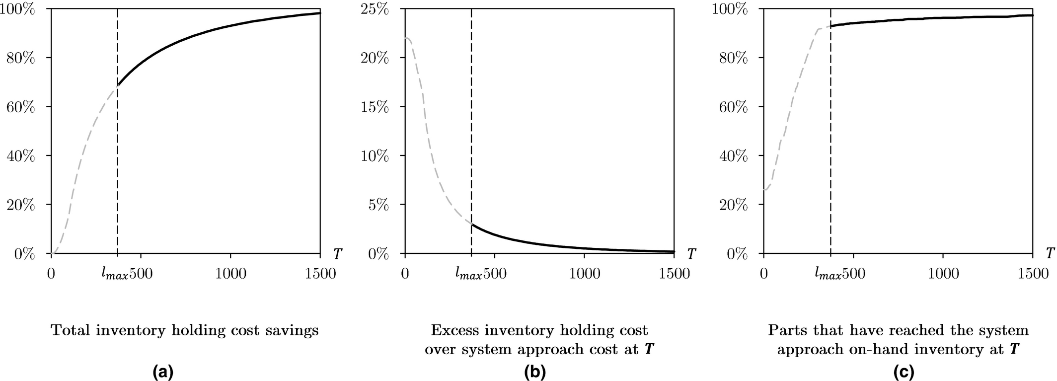
Effect of Planning Horizon
The length of an appropriate planning horizon depends on the goals of the company and the characteristics of the inventory system. Companies can, for example, set a maximum percentage 
To determine an appropriate planning horizon 


To reduce the inventory above budget after the transition, companies can decide on whether to extend the planning horizon
Conclusion
In this study, we have analyzed how the transition of inventory systems can be controlled when the inventory policy changes from an item approach to a system approach. We have shown that an uncontrolled transition results in severe violations of operational constraints, which can jeopardize the successful implementation of the system approach in practice. We have formulated an optimization problem that enables a smooth adaptation of base stock levels over time with the objective to maximize the average system fill rate without exceeding the inventory holding cost budget during the transition. We have presented two approaches to solve the problem. The first approach is based on decomposition and column generation and provides an upper bound and a well‐performing feasible solution to the maximization problem. However, it requires long runtimes for large‐scale inventory systems and long transition periods. The second solution approach is a heuristic that is based on marginal analysis. It is able to solve the transition of large‐scale inventory systems with very short runtimes. We have demonstrated the performance of both approaches in an extensive numerical study.
Our research provides important managerial implications. First, it raises awareness for the unique challenges companies have to face when optimizing an existing inventory system. In such situations, it is not only important to establish a new target state of the system but it is also important to consider the transition period. Second, we provide insights on why the inventory system performance might fall short of the target performance during a transition period and how severe this deterioration can be. Even if managers decide against transition period control and cope with the resulting disturbances instead, our research helps to understand the implications and to avoid wrong interpretations and actions. It might also reduce the stress put on responsible units within a company. Third, we provide a solution approach that enables companies to keep inventory cost within a budget during the transition period. We also provide guidance on how to choose an appropriate length for the transition period. The suggested controlled transition is easy to apply in practice as the recommended base stock levels during the transition period can be integrated in existing operational routines and ERP systems.
To maximize the average system fill rate without exceeding the inventory holding cost budget, we allow the base stock levels to change gradually during the transition period. If a gradual adaptation is not desired, our approach could be simplified to a single‐adjustment policy per item. Pinçe et al. (2015) have demonstrated that such a policy performs well for the base stock level transition of a single item in continuous‐time. Going forward, it would be interesting to analyze how such a policy performs in our multi‐item setting.
Even though we have focused on the introduction of the system approach in an inventory system that has been operated under the item approach before, our approach is suited for any adaptations of base stock levels in an inventory system that should eventually operate under a system approach. This makes our approach applicable for a broad range of situations, for example, if new information regarding demand or reliability of parts is available, unit holding costs change, parts are substituted, or new supply sources are explored. If resulting changes in base stock levels are not quickly reflected in inventory, controlling the transition is important and valuable.