Sage Journals: Discover world-class research

Abstract

We examine inventory decisions in a multiperiod newsvendor model. In particular, we analyze the impact of budget cycles in a behavioral setting. We derive optimal rational decisions and characterize the behavioral decision‐making process using a short‐sightedness factor. We test the aforementioned effect in a laboratory environment. We find that subjects reduce order‐up‐to levels significantly at the end of the current budget cycle, which results in a cyclic pattern during the budget cycle. This indicates that the subjects are short‐sighted with respect to future budget cycles. To control for inventory that is carried over from one period to the next, we introduce a starting‐inventory factor and find that order‐up‐to levels increase in the starting inventory.

Keywords

inventory management multiperiod budget cycle behavioral operations lab experiments

Introduction

Managing inventories to align supply with demand is critical for the financial performance of many firms (Eroglu and Hofer 2011, Hendricks and Singhal 2009, Steinker and Hoberg 2013). Most products are sold over multiple periods and can be replenished in regular intervals. Even though in many cases replenishment systems are automated, inventory managers still monitor stock levels over time, observe fluctuating demand, and place or adjust orders with suppliers as required. Therefore, the human effect is a crucial part of such replenishment systems (Bendoly et al. 2010, Boudreau et al. 2003, Gino and Pisano 2008).

Inventory managers typically face performance evaluations on a regular basis, e.g., based on monthly, quarterly, or yearly budget cycles. The most common budget cycle is the fiscal year, and firms generally aim to demonstrate higher performance toward the end of the fiscal year. This also holds for inventories, because investors have recently been found to pay particular attention to inventory metrics (Gaur et al. 2005, Kesavan et al. 2010), which can reveal important information about operational efficiency (Monga 2012) and future financial performance (Kesavan and Mani 2013). Prior literature has also shown that firms often engage in real earnings manipulation towards the fiscal‐year end to demonstrate better performance to the stock market (Roychowdhury 2006). In an inventory‐specific context, Lai (2008) found that retailers reduce inventories on average by 10% in the fourth fiscal quarter, even after correcting for sales timing. Hoberg et al. (2017) extended this analysis to manufacturing firms, which reduce inventories on average by 6% at the end of the fiscal year. These strong inventory reductions could serve as signals of efficiency.

Accordingly, an inventory manager who receives a bonus based on performance within the current budget cycle may have the incentive to optimize inventories toward the end of that cycle. Human decision makers may thus be short‐sighted and focus only on decisions and bonuses pertaining to the current budget cycle, mentally discounting future bonuses because they are temporally distant. Moreover, in some cases human planners will no longer be responsible for a given task in the following budget cycle, e.g., due to job changes. Therefore, it is possible that limited planning horizons and short‐sightedness result in the evaluation of these repeated incentives as single‐period incentives.

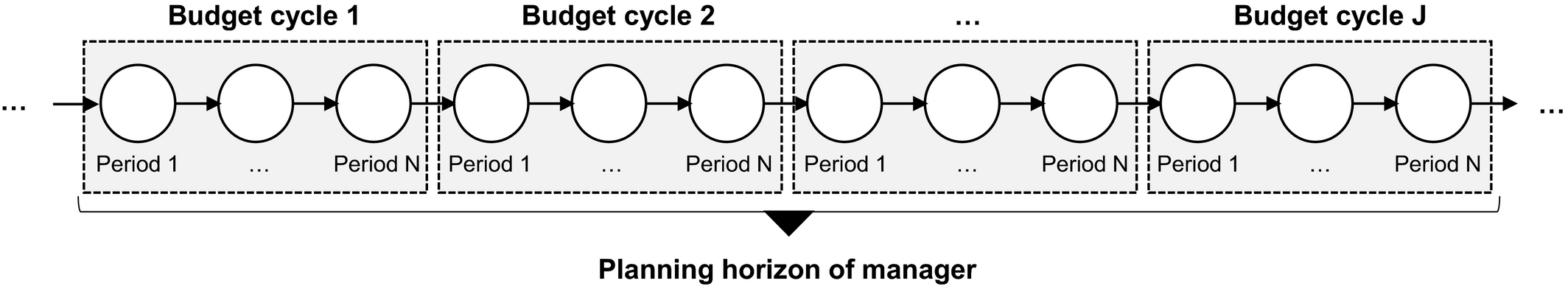
In this study, we analyze the effect of the budget cycle in a multiperiod inventory setting. Figure 1 outlines our stylized setting. A human decision maker is responsible for making inventory decisions over J·N periods. This relates to J budget cycles with each budget cycle consisting of N periods. In each period, a replenishment order is placed, demand is observed, and inventories are carried over to the next period. However, the human decision maker does not receive a formal incentive to optimize inventories in view of the budget cycle. She is incentivized by the total cash flow generated over all J·N periods. Using laboratory experiments, we explicitly analyze behavioral aspects in this multiperiod inventory management setting. Many behavioral studies have explored the impact of human behavior on inventory management using a single‐period model (for an overview of behavioral inventory management studies see, e.g., Becker‐Peth and Thonemann 2018).

Figure 1

Multiperiod Setting with Budget Cycles

The classic newsvendor setting typically serves as a basis for this stream of literature. From the perspective of financial performance metrics, the newsvendor model relates to a classic cash flow incentive: the decision maker faces random demand and has to determine the optimal inventory level to balance leftover inventory and lost sales at the end of the period. Remaining inventory is carried over from one period to the next. However, little is known about human behavior when the newsvendor model is extended to the multiperiod case, that is, to a setting in which starting inventory is present at the beginning of a period, the decision maker faces multiple periods with stochastic demand, and she has to make multiple order decisions. In addition, researchers have not investigated whether the framing of budget cycles does in fact affect the order decisions. Rationally, this should not be the case, because all bonuses in our setting simply accumulate over time and are not discounted in any way.

Against this background, the objective of our study is to investigate the factors that affect human decisions in multiperiod decision‐making. In particular, we examine how human planners react to starting inventories that are carried over from one period to another. Next, we investigate the impact of budget cycles and analyze the extent to which human decision makers adjust their ordering decisions during the budget cycle. Specifically, we derive the optimal order‐up‐to level to understand the decision of a fully rational decision maker. Next, we conduct a lab experiment to test the rational predictions and disentangle three behavioral factors that become relevant in our setting. We find that normatively irrelevant budget cycles have a significant impact on actual ordering behavior because decision makers focus too much on the current cycle and under‐weight the effects on future cycles.

Our research is closely related to two streams of research: (i) behavioral operations management, and (ii) finite‐horizon inventory models. The research on behavioral operations management provides one of the foundations of our paper. Behavioral research in general challenges the main underlying assumption of most operation management models: fully rational profit maximization by the decision maker. Deviations from this assumption can be categorized into two dimensions. The first is the use of an alternative utility function, including risk and loss aversion (Abdellaoui et al. 2007, Tversky and Kahneman 1991) or preferences in addition to or different from the absolute monetary payoff, e.g., stock‐out aversion. The second dimension is the inability to maximize the utility function: This includes decision heuristics (Tversky and Kahneman 1974) and bounded rationality (Simon 1955).

Starting with Schweitzer and Cachon (2000), recent contributions to the literature have considered actual stocking decisions in the newsvendor setting using laboratory experiments. Testing different theories, these studies have provided evidence for various decision biases that are partly general and partly context dependent. The most striking observation, which is consistent across nearly all follow‐up studies, is the so‐called pull‐to‐center effect. In the classical newsvendor problem, optimal stocking quantities are above mean demand for high profit margins and below mean demand for low profit margins—the critical fractile solution (Arrow et al. 1951). In laboratory experiments, human decision makers actually order more (less) than mean demand in high‐ (low‐) margin settings, but they significantly deviate from the optimal order quantities. The adjustment upward (downward) from mean demand to the optimal order quantities is insufficient; the order quantities are between mean demand and the optimal quantities—they are pulled to center (Schweitzer and Cachon 2000). This effect decreases little over time (Bolton and Katok 2008), and students as well as managers exhibit this decision bias in the lab (Bolton et al. 2012).

Based on this observation, explanations such as risk and loss aversion/seeking have been ruled out as (stand‐alone) explanations for the decision biases, because such preferences would lead to similar deviations in the high‐ and low‐profit cases, e.g., risk‐ or loss‐averse decision makers would order less in both cases (Becker‐Peth et al. 2018, Eeckhoudt et al. 1995, de Vericourt et al. 2013, Wang and Webster 2009 analyze how risk preferences affect human newsvendors in more detai). To explain the observed ordering pattern, various theories have been tested, including bounded rationality (Su 2008), mean anchoring (Schweitzer and Cachon 2000), prospect theory (Long and Nasiry 2014), and ex‐post inventory error minimization (Ho et al. 2010, Kremer et al. 2014). Although the literature has found support for each of their explanations, the trade‐off between these theories has yet to be analyzed sufficiently. Other studies have analyzed context‐specific decision biases. Katok and Wu (2009) found significant differences in ordering behavior between equivalent buyback and revenue‐sharing contracts. Becker‐Peth et al. (2013) found specific mental accounting effects (Thaler 1999) in the buyback contract, and Kremer et al. (2010) found a stronger anchoring on mean demand in the newsvendor setting compared to an equivalent lottery choice task. In contrast to our paper, this stream of the literature has focused on the single‐period newsvendor setting without inventory carryover.

In the domain of multiperiod inventory settings, a stream of research has investigated the well‐known beer game, which is a multistage inventory system (e.g., Croson and Donohue 2006, Croson et al. 2014, Sterman 1989). These studies have described the bullwhip effect, which can be attributed to both structural deficits of the system and behavioral factors, e.g., decision makers’ practice of under‐weighting the supply line. Our setting differs substantially from this one. First, we do not consider backlogs but use a lost sales system. Second, we abstract from lead times, so there is no supply line that could be under‐weighted. Additionally, the literature on the beer game setting has focused strongly on demand variability amplification across multiple players and has paid less attention to the multiperiod inventory decision‐making of individuals, which is the focus of our paper.

Other studies of multiperiod inventory decisions include Hartwig et al. (2015), who analyzed strategic inventories in a two‐period setting but with deterministic demand. The newsvendor model with transshipments (for theoretical studies see, e.g., Dong and Rudi 2004, Sošić 2006 has been developed by a stream of literature that is based on the two‐period newsvendor model. However, in that setting, the second decision is not an ordering decision under uncertainty but rather a filling up/selling decision with deterministic quantities, and little work has examined the behavioral aspects of decision makers in this setting.

Using a setting rather similar to ours, Katok et al. (2008) examined a multiperiod setting under a service level agreement, but they focused on the effect of the review periods and the size of the service level bonus rather than on differences of actual order decisions between periods. Additionally, they used the order‐up‐to level as the decision variable, whereas we use order quantities (the details of our setting are described below).

In terms of the psychological literature, decision‐making in our setting is related to choice bracketing, which is defined as “the grouping of individual choices together into sets” (Read et al. 1999, p. 172). When decision makers act in a budget cycle environment, they may be affected by the cyclic frame. Kahneman and Lovallo (1993) argued that “people tend to make decisions one at a time, and […] they are prone to neglect the relevance of future decision opportunities” (Kahneman and Lovallo 1993, p. 23). Similarly, Rabin and Weizsäcker (2009) argued that “a decision maker who faces multiple decisions tends to choose an option in each case without full regard to the other decisions and circumstances that she faces” (Rabin and Weizsäcker 2009, p. 1508). Regarding financial investments, Benartzi and Thaler (1995) related this effect to differences between evaluation periods and planning periods. Investments for a pension plan (with a planning horizon of 30 years or more) are affected by the yearly evaluation reports, e.g., those provided by the insurance companies. This results in actions of decision makers that optimize their investment plan for the upcoming year (evaluation period) while under‐weighting the long‐term effects (planning horizon) (Benartzi and Thaler 1995). Although the terms used in the papers differ (e.g., narrow frames or isolated choices in Herrnstein and Prelec 1992, Kahneman and Lovallo 1993), all the terms refer to the effect of choices being “made with an eye to the local consequences of one or few choices” (Read et al. 1999, p. 172, calling it narrow bracketing). Having a budget cycle frame in the experiment, we expect similar effects to be present in the setting. In this study, we refer to this effect as short‐sightedness.

In light of the aforementioned literature, our study makes a threefold contribution. First, we analyze the effect of the cash flow incentive on inventory decisions in a multiperiod (finite horizon) setting and determine that optimal order‐up‐to levels decrease towards the end of the planing horizon. Second, we find that starting inventory plays an important role when human subjects decide on order quantities. Subjects seem to under‐weight the available starting inventory when making their ordering decisions. We find that a unit of starting inventory increases the order‐up‐to level by 0.324 units. Third, we analyze how budget cycles affect decision‐making in the multiperiod setting. We find that order‐up‐to levels follow a cyclic pattern over time: orders are higher in the early periods and lower in the later periods of a budget cycle. This is driven by short‐sighted behavior, because human decision makers focus on the current budget cycle and disregard future periods. We test different lengths of budget cycles and different frames and find consistent short‐sightedness in ordering behavior in all settings.

The remainder of the study is structured as follows. In section 2, we formulate mathematical models for rational and behavioral decision‐making. In section 3, we analyze behavioral decision‐making based on single‐period and multiperiod laboratory experiments. In section 4, we conclude and discuss our findings. All proofs can be found in the Appendix.

Decision‐Making

In this section, we formulate the mathematical model for the classic cash flow incentive scheme. The cash flow incentive is used to analyze both rational and behavioral decision‐making. We then describe the sequence of events and derive the rational single‐period model (section 2.1), which serves as a building block for the rational multiperiod model (section 2.2) and the behavioral multiperiod model that we develop subsequently (section 2.3). Products are non‐perishable and have an infinite horizon. However, managers are typically held accountable for their performance over the budget cycle, which is a finite horizon (Thomas 2005). In our single‐period model, the manager has to make decisions for only one period of the infinite horizon. Analogously, in the two‐period model, the manager has to make decisions for two consecutive periods of the infinite horizon. Finally, in the multiperiod model, the manager has to make decisions for multiple budget cycles with two periods each. Accordingly, we assume a finite incentive horizon, which is in line with the short‐term incentive structures in place in many companies that have incentives linked to specific time intervals, e.g., a month, quarter, or year.

Rational Single‐Period Model

The manager operates under an order‐up‐to level policy according to which she brings the inventory level to S at the beginning of the single period. The customer demand ξ is stochastic, with p.d.f. f(ξ) and c.d.f. F(ξ). The unit sales price is r, and the unit purchase cost is c. Excess inventory at the end of the period incurs a unit holding cost h that reflects the physical inventory holding fee charged by a logistics service provider. Our model assumes lost sales; that is, unfulfilled demand does not carry over to the next period but is lost. Motivated by the work of Zipkin (2008) and Bharadwaj et al. (2002), we focus on a lost sales problem. More specifically, Bharadwaj et al. (2002) showed that only 15% of consumers will delay their purchase in the event of a stock‐out. Our model assumes no unit shortage costs for lost sales.

In our paper, the manager makes inventory decisions under a cash flow incentive. The objective function for the cash flow incentive includes the revenue from sales, the purchasing cost for all products purchased, and the holding cost. The cash flow is defined as

C F (S) = r {(S, ξ)}^{-} - c S - h {(0, S - ξ)}^{+},

where S is the order‐up‐to level. We use the following notation:

{(a, b)}^{-} = m i n (a, b)

and

{(a, b)}^{+} = m a x (a, b)

. Therefore,

{(S, ξ)}^{-}

is the sales quantity (minimum of order‐up‐to level and demand), and

{(0, S - ξ)}^{+}

is the excess inventory at the end of the period.

Note that the cash flow is directly affected by units bought but not sold in the period. Furthermore, we assume that the initial inventory is zero, while the model can be easily adjusted otherwise. The expected objective function for the single‐period cash flow incentive is shown in Equation 2.

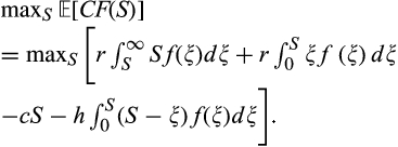
\begin{matrix} max_{S} E [C F (S)] \\ = max_{S} [r \int_{S}^{\infty} S f (ξ) d ξ + r \int_{0}^{S} ξ f (ξ) d ξ \\ - c S - h \int_{0}^{S} (S - ξ) f (ξ) d ξ] . \end{matrix}

In the analytical model and for simplicity of presentation, we assume that the demand follows a continuous uniform distribution U[0,1]. If demand follows a continuous uniform distribution U[0,1], then we can easily show that the optimal order‐up‐to level is

S^{*} = \frac{r - c}{r + h}

. Note that for the numerical analyses, we use a continuous uniform distribution U[0,100], because it intuitively relates to the laboratory setting.

Rational Multiperiod Model

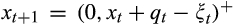
In this section, we extend our single‐period model to a multiperiod inventory decision problem, in which the manager operates under an order‐up‐to level policy according to which she observes the initial inventory level

x_{t}

at the beginning of period t and brings it to level

S_{t}

S_{t} > x_{t}

by placing an order

q_{t} = {(0, S_{t} - x_{t})}^{+}

. If the optimal cash flow profit from period t onwards is now denoted as

{\hat{CF}}_{t} (x_{t}, S_{t})

, then we can use the following recursive expression:

\begin{matrix} {\hat{CF}}_{t} (x_{t}, S_{t}) & = max_{S_{t}} [r \int_{x_{t} + q_{t}}^{\infty} (x_{t} + q_{t}) f (ξ_{t}) d ξ_{t} \\ + r \int_{0}^{x_{t} + q_{t}} ξ_{t} f (ξ_{t}) d ξ_{t} - c q_{t} \\ - h \int_{0}^{x_{t} + q_{t}} (x_{t} + q_{t} - ξ_{t}) f (ξ_{t}) d ξ_{t} \\ + {\hat{CF}}_{t + 1} (x_{t + 1}, S_{t + 1})], \end{matrix}

where

x_{t + 1} = {(0, x_{t} + q_{t} - ξ_{t})}^{+}

. See Zipkin (2000,2008) for a detailed discussion of the recursive equations and standard transformations for the lost sales problem. For the multiperiod model, a closed form solution is not possible. Zipkin (2000,2008) provided a detailed discussion of solution techniques and heuristics based on state reduction for lost sales models. We can derive a closed form solution for the special case of two periods.

Proposition 1

For a two‐period model, the optimal order‐up‐to level for the first decision

S_{1}^{*} = \frac{\sqrt{r^{2} + 2 h r + h^{2} - 2 c h - c^{2}} - h}{r + h}

is higher than that for the second decision

S_{2}^{*} = \frac{r - c}{r + h}

(which is equivalent to the single‐period decision).

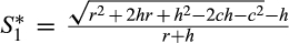
Figure 2 illustrates the numerical optimal order‐up‐to levels for different horizon lengths (N = 1,2,4, and 8). For this analysis, we use r = 20, c = 7.5, and h = 5. Figure 2 shows that the optimal order‐up‐to level gradually decreases for the last two decisions (

S_{N}

and

S_{N - 1}

). The intuition behind this decrease is that the overage costs are higher for these periods, because there are no further opportunities to sell leftover products in later periods.

Figure 2

Optimal Order‐Up‐To Levels

Corollary 1

For a multiperiod model, the optimal order‐up‐to levels of the last two periods are equivalent to the two‐period model.

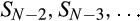
It is also evident that the order‐up‐to level increases once more for earlier decisions (for

S_{N - 2}, S_{N - 3}, \dots

for N = 4 and N = 8) but then stays constant at the high level. More specifically, the order‐up‐to levels

S_{N - 2}, S_{N - 3}, \dots

approach the level of the infinite horizon model. Having an infinite horizon, the optimal order‐up‐to level (base stock policy) is (Porteus 1990)

S_{\inf}^{*} = \frac{r - c}{r - c + h} .

For the numerical example in Figure 2, the optimal order‐up‐to level is

S_{\inf}^{*} = 71.4

. We conclude that the end‐of‐horizon effect is relevant only for the last (two) decisions in our setting.

Behavioral (Short‐Sighted) Multiperiod Model

The previous section analyzed rational decision‐making in the context of a multiperiod inventory setting. Following the classical operations management approach, we optimized our decision model and derived normative predictions for the optimal inventory decision for our setting. Our solution can be implemented into computerized optimization protocols. In practical settings, human decision makers often do not make inventory decisions according to the optimization models.

The growing field of behavioral operations management addresses this issue and incorporates human decision‐making into operations management models. In this section, we follow this research stream and analyze our setting from a behavioral perspective. Further, challenging the assumption of fully rational expected‐profit‐maximizing decision makers, we discuss which behavioral aspects may affect inventory decisions in our setting.

Numerous studies have analyzed actual human decision‐making in the context of inventory decisions (see Becker‐Peth and Thonemann 2018, for a comprehensive overview of existing behavioral newsvendor literature). Focusing mainly on the single‐period newsvendor, the consistent observation is that human decision makers do not order according to expected‐profit‐maximizing predictions. The reasons for this are manifold and include bounded rationality and alternative preferences.

Regarding human decision makers in realistic settings that involve multiperiod inventory decisions, there is a crucially important observation that should be captured in a decision model.

Many incentive systems for real‐world managers focus on the performance during a budget cycle, e.g., the year‐end bonus of a decision maker is based on the annual cash flow achieved within that year. Consider, for example, a product/inventory manager who has to place monthly orders for a certain (non‐perishable) product. At the end of the year, she will receive a bonus based on her yearly performance, e.g., the cash flow achieved with her product.¹

Rationally, such a cyclical incentive structure should not affect decision‐making. Fully anticipating the effect of current decisions on overall/future performance, decision makers should act according to the model described in the previous setting, even under such budget‐cycle‐bonus contracts. However, two factors may lead to deviations from the prediction of the previous section.

First, decision makers receiving the bonus at the end of the budget cycle may discount the future payments with a certain discount factor α; that is, future money is less valuable than recent money. This kind of modeling is also related to the financial literature on discounting future income (Brealey et al. 2006, Federgruen and Zipkin 1986). In the yearly payment example mentioned above, payments of future years are discounted, e.g., due to interest rates. In the lab experiment we consider, such delayed payments are not relevant, because there is no real time difference and no discounting.

However, a (second) behavioral bias affects decision‐making in a very similar way, and we expect it to hold in the lab setting. Decision makers focusing on the recent budget cycle may under‐weight the effect of the current cycle’s decisions on the following cycle. In our setting, reframing a decision task of 16 inventory decisions as 8 times 2 decisions (i.e., eight years with two decisions per year) can be seen as an example of inducing a narrow frame (Kahneman and Lovallo 1993); see the introduction for a more detailed description. Although decision makers are aware that they are making 16 decisions, the budget cycle frame may prevent them from fully considering the effects of the current decision on decisions in later years. We refer to this behavior as short‐sightedness: decision makers do not take all future effects into consideration when making an ordering decision.

Please note that products (and the company) may have an infinite planning horizon. However, the planning horizon for real‐world managers (and for the subjects in our lab experiments) is usually finite (e.g., due to job rotation or fixed‐term employment contracts). Therefore, it is appropriate to assume a finite horizon. However, if we assume an infinite horizon, the behavioral effects remain essentially the same (except for the last two periods).

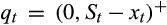
Consider that there are N decisions per budget cycle, e.g., 12 monthly decisions, and the bonus is paid only at the end of the year; then, the total yearly cash flow consists of the sum of the monthly cash flows of that year. Technically, we model the short‐sighted behavior as follows: decision makers discount all future‐year profits when making decisions in a certain budget cycle (e.g., decisions in periods t = 1,…,N are in the first budget cycle, decisions in periods t = N + 1,…,2N are in the second budget cycle, etc.). Given this notation, the budget cycle is then defined as

j = ⌈ \frac{t - 1}{N} ⌉

, where j = 1 is the first budget cycle, etc. Therefore, if we are currently in period t, which belongs to the

j^{th}

budget cycle, then we define the cash flow from period t onwards

\tilde{C F_{t}}

as seen in the following equation, where

C F_{t}

is the actual cash flows as defined above (note that we have suppressed the notation

(x_{t}, S_{t})

for the sake of simplicity).

\tilde{C F_{t}} = \sum_{k = 0}^{j N - t} C F_{t + k} + α \sum_{k = j N - t + 1}^{T - t} C F_{t + k}

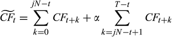
The first sum represents all the remaining decisions to be made within the current budget cycle, whereas the second sum includes all remaining decisions to be made within the subsequent budget cycles until the end of the time horizon, where T is the total number of decisions to be made (having J budget cycles, we have J·N = T periods/decisions). We formulate our model in this way (one discount factor for all decisions in upcoming budget cycles) because this may also be relevant in our experimental study. Technically, we solve the problem using backward induction, and we denote the optimal behavioral order‐up‐to level that maximizes Equation 5 as

S_{t}^{α}

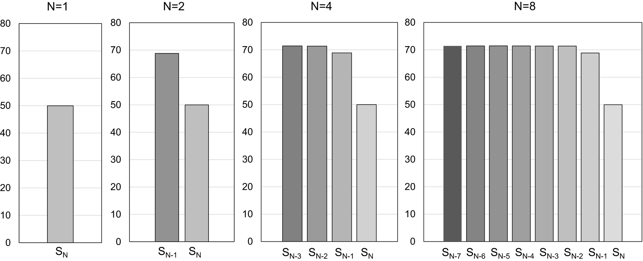
The analysis of the order‐up‐to levels shows a very interesting pattern. Figure 3 illustrates the predicted decisions for different discounting factors α for a setting with two periods/decisions per budget cycle for a horizon of eight budget cycles and for a setting with four decisions per budget cycle for a horizon of four years. Therefore, both settings have 16 decisions in total. The gray bars illustrate the first decisions in each budget cycle, whereas the white bars illustrate the second decision in each budget cycle.

Figure 3

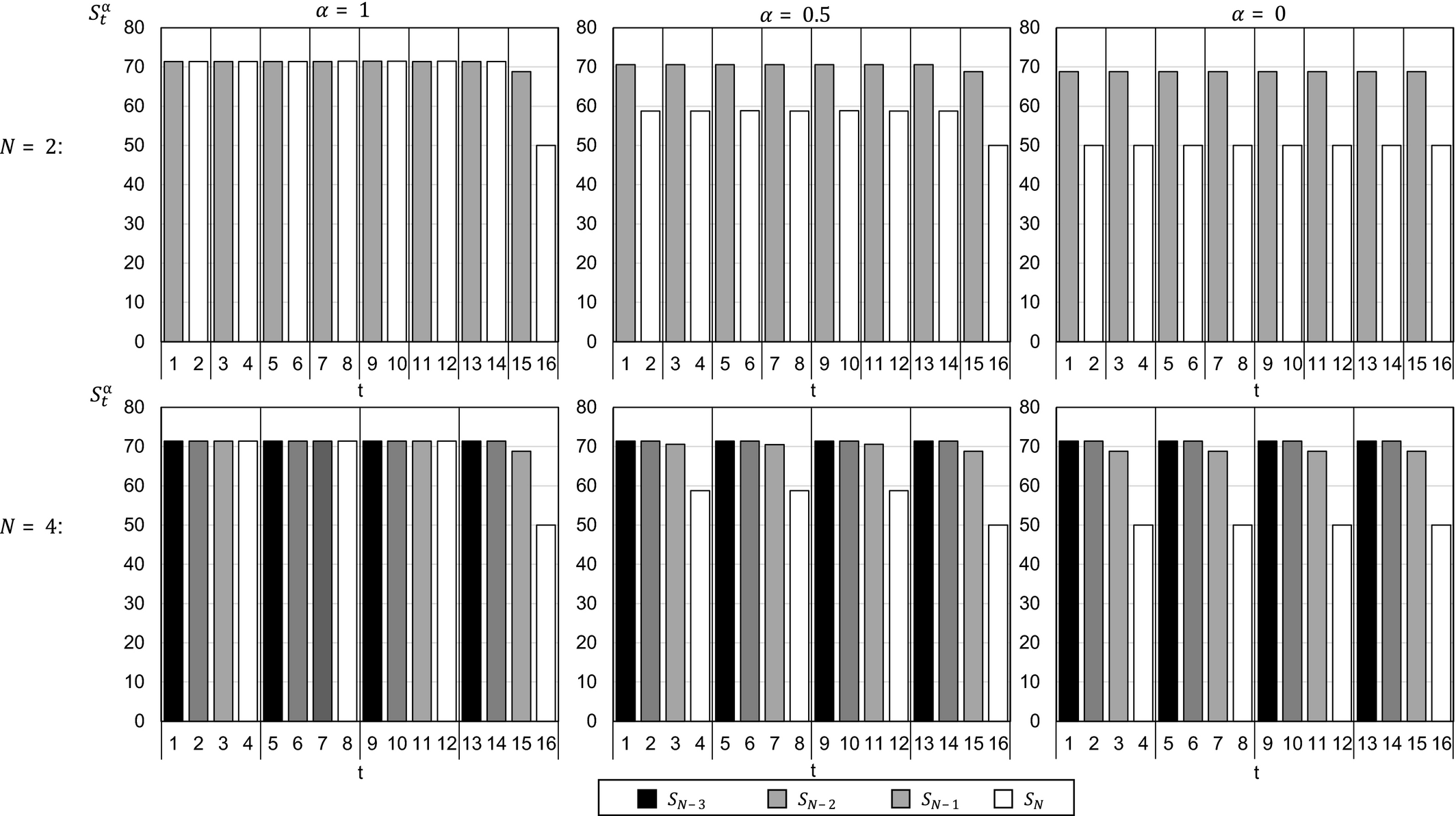
Optimal Order‐Up‐To Levels (numerical analysis) for Short‐Sighted Decision Makers Focusing on Budget Cycles

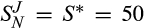
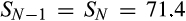
We first observe that the decisions in the last budget cycle are equivalent for different values of α because there is no future effect at all, so there is no difference in future discounting. Essentially, the order‐up‐to level for short‐sighted decision makers in the last budget cycle with N decisions per budget cycle is equivalent to the rational N‐period decision model.

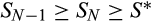
With respect to earlier budget cycles (j < J), we observe that short‐sightedness leads to a cyclic decreasing pattern of the order‐up‐to levels towards the end of the budget cycle. The last decision in a budget cycle

S_{N}

decreases substantially in α, and

S_{N - 1}

also decreases in α, but to a smaller extent. For α = 0, the decisions for all budget cycles are equivalent to the N‐period decision model (equivalent to Figure 2 with N = 2 repeating itself in each cycle), because the decision maker acts as if the horizon ends after the current budget cycle. For α = 1, the graph corresponds to Figure 2 with N = 16.

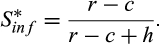
Regarding the N = 4 setting, we see that

S_{N - 2}

and

S_{N - 3}

are not affected by α (see also the normative N = 4‐period decision model in Figure 2). Additionally, for α = 0, the graph corresponds to a repeated Figure 2 with N = 4.

Experimental Design

Our setting differs from those of previous studies because it is a multiperiod setting. This leads to two main factors that may affect decision‐making by human subjects in the laboratory. First, for multiperiod products, inventory is carried over, yielding starting inventory at the beginning of the next period. This has not been addressed in previous behavioral operations literature. Therefore, we design an experiment to test whether starting inventory has an effect on the order‐up‐to level. Second, we design an experiment to test the aforementioned short‐sighted behavior in the multiperiod setting.

Study 1: Single‐Period Model with Starting Inventory

Most existing behavioral studies use settings without starting inventory and ask the subjects to determine order quantities explicitly. For these studies, the order quantity equals the order‐up‐to level. However, for our multiperiod model, the ending inventory from a period is carried over to the next period and serves as the starting inventory for the next period. Accordingly, this will frequently violate the assumption of no starting inventory.

In our setting, the optimal inventory policy is an order‐up‐to policy. This is equivalent to an order quantity policy whereby the starting inventory is deducted from the optimal order‐up‐to level. Assuming no starting inventory, the order quantity is equivalent to the order‐up‐to level. To keep our experiments similar to the existing literature, we use the order quantity as the subject’s decision variable. Therefore, decision makers have to account for possible nonzero starting inventory and deduct this from their targeted order‐up‐to level. Rationally, the order‐up‐to level should be the same for different starting inventories as long as the starting inventory is below the optimal order‐up‐to level. If the starting inventory is above the optimal order‐up‐to level, decision makers should order zero units. In Study 1, we analyze the effect of starting inventory on the order‐up‐to level in the single‐period model.

Laboratory Design

To analyze whether starting inventory affects the order‐up‐to levels of human decision makers, we conduct an experiment in which the starting inventory is altered while the optimal order‐up‐to level is held constant. To keep the setting as simple as possible, we focus on a single‐period model to analyze the effect of starting inventory.

The decision maker purchases products at a unit purchasing cost c before the selling period. Demand is discrete and uniformly distributed between 1 and 100. Similar discrete uniform demand distributions are commonly used in experimental studies (e.g., Bolton and Katok 2008, Bolton et al. 2012, Schweitzer and Cachon 2000). If a product is sold, the decision maker receives a unit revenue r. If a product is not sold, it is stocked in inventory and induces a unit holding cost h. In our experiment, we set r = 20, c = 7.5, and h = 5. This results in an optimal order‐up‐to level of 50 units in the single‐period model. The reason for this choice is to address the possible pull‐to‐center effect. Previous research has indicated that subjects anchor on mean demand and that order quantities are pulled towards mean demand (Bolton and Katok 2008, Bolton et al. 2012, Schweitzer and Cachon 2000). With our parameters, the optimal order‐up‐to level equals the mean demand, and deviations from the optimal order‐up‐to level therefore cannot be explained by mean anchoring.

To keep our experiments similar to the existing behavioral operations literature, the decision makers are asked to determine order quantities. To test the effect of starting inventory on the decisions, we varied the starting inventory. We chose a starting inventory of

I_{START} = 0, 10, 20, 30, 40, 50, 60, 70

units. Starting inventories smaller than or equal to the optimal order‐up‐to level of 50 units are natural choices and should lead to order quantities that result in an order‐up‐to level of 50 units. For starting inventories equal to or above 50 units, the optimal ordering quantity is zero (recall that negative orders are not permitted). We explicitly included these values to test the effect of setting the starting inventory above the actual targeted order‐up‐to level. This may also happen in the multiperiod model if the optimal order quantity is smaller in the upcoming period than in the previous period and the actual demand in the previous period is relatively small. Using a starting inventory of zero allows us to calibrate the order‐up‐to levels to the actual (non‐affected) order‐up‐to level that the subjects want to achieve.

Subjects faced each starting inventory twice, resulting in a total of 16 decisions. We randomized the sequence of starting inventory levels to avoid ordering effects. The only exception was that we used one of the

I_{START} = 0

settings as the first round to have a non‐affected decision for this starting inventory. This enables a better calibration of the decision makers’ targeted order‐up‐to level.

In our experiment, the decision task is more complex than in the simple newsvendor setting. Therefore, we provide decision support in the form of a bar chart. This chart showed the actual starting inventory, and the subjects could enter different possible order quantities. The screen then stated the inventory level after the order (i.e., the order‐up‐to level). The bar chart also visualized this and displayed the expected sales and resulting expected inventory level after demand realization. This should have helped the decision makers to evaluate the effect of their order quantity on the expected revenues and the expected inventory costs. The experiment was implemented in Z‐Tree (Fischbacher 2007); screenshots can be found in the Online Appendix. After each round, demand was realized and the subjects saw their actual performance.

We conducted the experiments at the Cologne Laboratory for Economic Research (CLER). We invited 14 students via an online recruitment system (ORSEE); all of them were master’s students with majors in business administration or economics. At the beginning of the experiment, students received written instructions. The instructions explained the setting and the decision task (instructions are contained in the Online Appendix). After reading the instructions, the subjects had to answer control questions about the experiment. They could make as many attempts as needed to answer the questions but could continue with the experiment only after correctly answering all questions. Having 16 decisions, subjects were paid according to their average performance over all 16 rounds; that is, in the cash flow model, subjects were paid based on the average cash flow achieved in the experiment. Overall, the session lasted approximately 60 minutes, and the subjects earned an average of around 15 euro.²

Experimental Results

To analyze the inventory decisions of the subjects in the lab experiments, we first calculate the actual order‐up‐to level of the decision maker. Figure 4 shows the mean order‐up‐to levels for the different starting inventories. The horizontal line indicates the optimal order‐up‐to levels given the starting inventory.

Figure 4

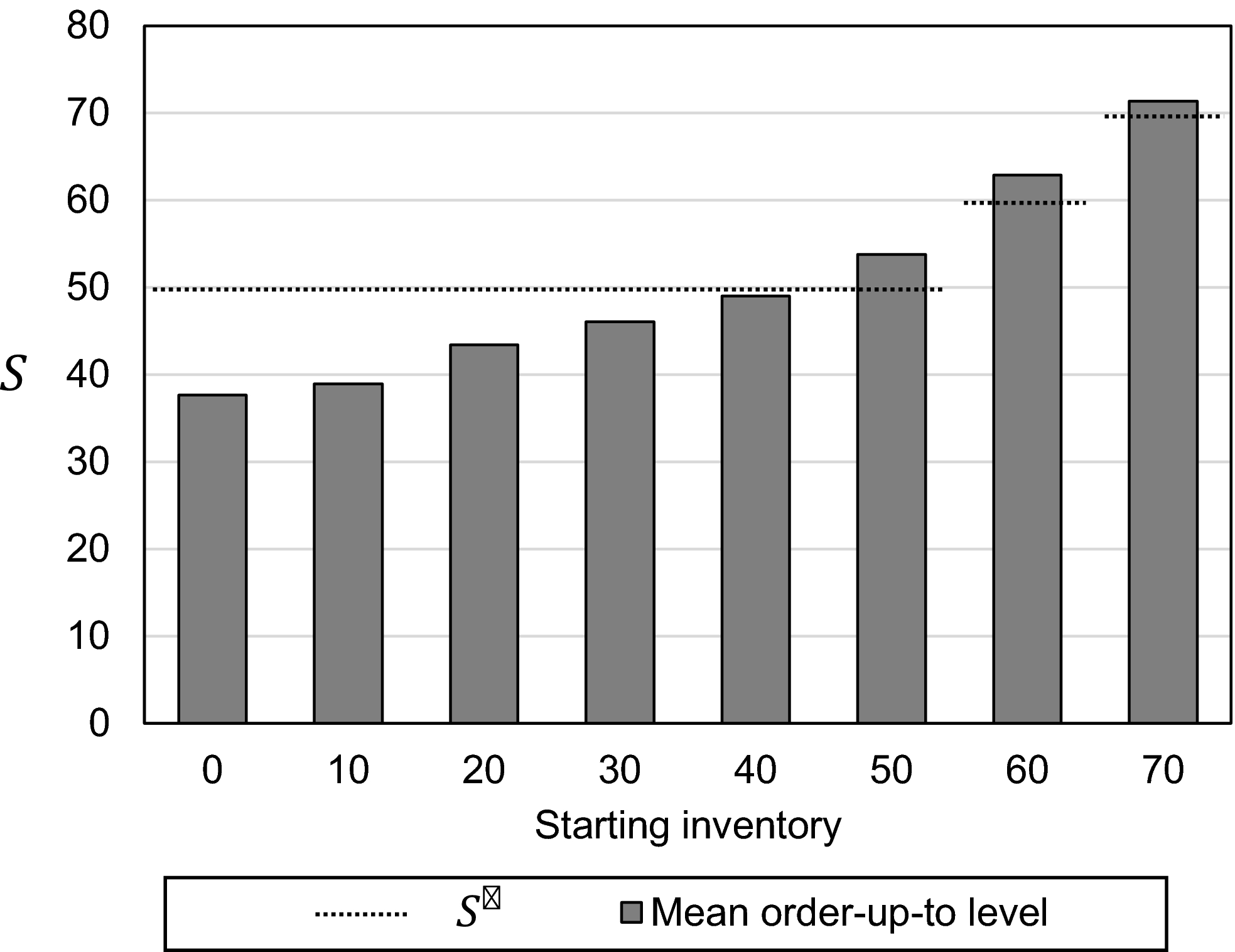
Empirical Mean Order‐Up‐To Levels for Different Starting Inventories

First, we observe that the order‐up‐to level is below the optimal order‐up‐to level for most of the starting inventories. For zero starting inventory, the mean order‐up‐to level is only 37.7 units, which is significantly different from the optimal level of 50 (p < 0.001). There are many possible reasons for this. Risk and loss aversion are natural candidates for an explanation, but over‐weighting inventory costs (e.g., leftover aversion) may also drive this behavior.

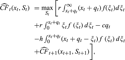
Second, we observe that the order‐up‐to level increases in the starting‐inventory level. For example, the mean order‐up‐to level for starting inventories of 50 units is 53.8 units, which is significantly greater than the 37.7 for zero starting inventory (p = 0.001, Wilcoxon signed‐rank test). This effect may be driven by the fact that the starting inventory is above the actually targeted order‐up‐to level, and we need to control for this effect. Adjusting the approach of Sterman (1989) and Croson and Donohue (2006) (who estimate the under‐weighting of pipeline inventory) to the starting inventory in our setting, the order quantity q of a subject is

q = max (0, β_{0} + β_{1} I_{START}) .

Adjusting this to the order‐up‐to level, we receive

S_{i} = max (I_{START}, β_{0} + β_{1}^{'} I_{START}),

where

β_{1}^{'}

relates to

β_{1}

from above with

β_{1}^{'} = β_{1} + 1

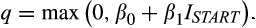
The expected‐profit‐maximizing solution equals

β_{0} = 50

and

β_{1}^{'} = 0

. We estimate the parameters individually for each subject using a bootstrapped maximum‐likelihood estimation with 100 replications per subject (each estimation contains N = 16 data points). Additionally, we perform a pooled estimation (N = 224) with subject‐specific clusters (again bootstrapped with 100 replications). Table 1 presents the estimated parameters per subjected and pooled. It shows that

β_{1}^{'}

is significantly > 0 for eight out of 14 subjects and

β_{0}

is significantly smaller than 50 for 10 out of 14 subjects. Pooled, the subjects under‐weight the starting inventory by 0.324 (significantly > 0, p < 0.001) and have a

β_{0} = 36.7

Table 1

Estimation Results of Inventory Weighting Parameters

ID	$β_{0}$	p‐value	$β_{1}^{'}$	p‐value	ID	$β_{0}$	p‐value	$β_{1}^{'}$	p‐value
1	30.1	0.000	0.429	0.274	8	40.0	0.000	0.000	0.999
2	27.6	0.000	0.529	0.000	9	39.8	0.044	0.293	0.038
3	54.8	0.061	0.380	0.000	10	34.8	0.000	0.393	0.000
4	44.0	0.164	0.414	0.007	11	19.1	0.000	0.696	0.000
5	43.0	0.031	0.050	0.782	12	45.0	0.481	−2.000	0.262
6	43.0	0.207	0.050	0.930	13	36.5	0.000	0.271	0.008
7	36.5	0.001	0.331	0.017	14	43.5	0.207	−0.150	0.581
Pooled	36.7	0.000	0.324	0.000

Note:

Bootstrapped MLE with 100 replications each. Parameters significantly different from normative predictions (

β_{0} = 50, β_{1}^{'} = 0

) are in bold (p < 0.1).

For robustness, we conducted two additional analyses. First, we consider only those rounds for which the actual order quantity is > 0. Figure 5 shows the mean order quantities for the different starting inventories. We observe that the order quantities are not sufficiently reduced to compensate for the increasing starting inventories. Using the fixed‐effect regression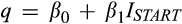

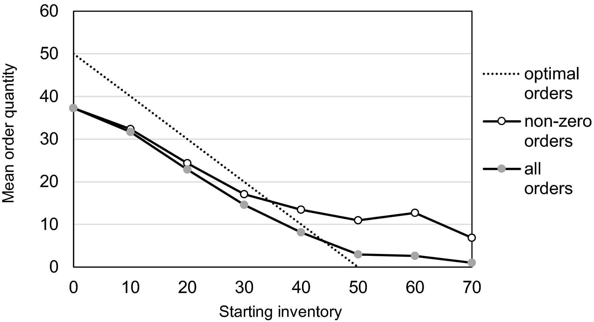
q = β_{0} + β_{1} I_{START}

shows that the coefficient for the starting inventory is significantly > −1 (

β_{1} = - 0.513

for nonzero orders, and

β_{1} = - 0.675

for all orders if

I_{START} \leq 50

, with p < 0.001 for both analyses).

Figure 5

Empirical Order Quantities for Different Starting Inventories

Second, we consider the order‐up‐to level for the decisions when starting inventory is zero and assume that these settings show the unbiased order‐up‐to level. For each subject, we exclude those periods when the starting inventory is above the order‐up‐to level of the zero‐starting‐inventory case. This excludes all settings in which we expect subjects to order zero units. The results are comparable to the previous results, with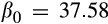

β_{0} = 37.58

(smaller than 50, p < 0.01) and

β_{1}^{'} = 0.251

(> 0, p < 0.01).

Endogenous Starting Inventory: The Two‐Period Case

In the experiment in Study 1, the starting inventory was externally given by us. Because this is rather artificial, we additionally conducted an experiment with two consecutive decisions with inventory carryover. This also serves as a robustness check if the effect is still visible in a more complex setting. Using the same cost parameters and demand distribution as above, the second period of that setting mimicked the previous experiment, with the difference that starting inventory was now a result of their first order decision and random demand realization. Subjects played eight rounds of these two decisions (28 subjects participated in that experiment).³ The normative predictions for that setting are visualized in the second graph (N = 2) of Figure 2. We conduct the same analyses as in Study 1 for the second (and therefore last) decision per round. The results are robust: subjects also under‐weight the starting inventory (

β_{1}^{'} = 0.124, p < 0.001

The results show that having higher starting inventories increases order‐up‐to levels even when starting inventories are below the optimal order‐up‐to level. Previous studies have not analyzed this bias, because they have not used multiperiod settings or starting inventories. This result is very interesting and implies that decision makers do not follow an order‐up‐to policy when they are asked to determine order quantities.

Study 2: Multiperiod Case

To examine a second behavioral aspect, we test whether and how short‐sightedness affects decision‐making in the context of multiperiod inventory decisions. Based on our analysis in section 2.3, we design an experiment which relates to the empirical setting with budget cycles. Here we relate a budget cycle to a year with two periods per year. Bonuses are awarded annually, and total payout is calculated as the sum of the annual cash flows.

Laboratory Design

The design of Study 2 is related to the previous experiment. The decision maker purchases products at a unit purchasing cost c before the selling period. Demand is discrete and uniformly distributed between 1 and 100. If a product is sold, the decision maker receives a unit revenue r. If a product is not sold, it is stocked in inventory and induces a unit holding cost h. Again, we use r = 20, c = 7.5, and h = 5.

The main difference of Study 2 is that subjects played 16 consecutive rounds; that is, the leftover inventory of round t is the staring inventory of round t + 1. Subjects made 16 decisions consecutively, seeing the demand realizations and leftover inventory of the previous round. The subjects were paid according to the overall cash flow obtained over all 16 decisions.

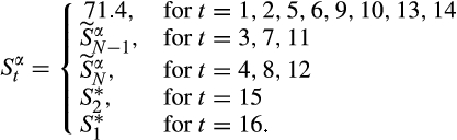
The rational expected‐profit‐maximizing order‐up‐to levels therefore follow the pattern described in Corollary 1. The left graph of Figure 3 shows the rational predictions (α = 1) for our setting. Subjects should have an order‐up‐to level of approx.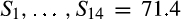

S_{1}, \dots, S_{14} = 71.4

for the first 14 decisions and then decrease the order‐up‐to level to

S_{15} \approx 68.8

and

S_{16} = 50

In total, we designed four treatments to test short‐sighted behavior in the lab, as shown in Table 2. In Treatment 1, we display all 16 decisions on one screen. Subjects place order quantities for a specific round and see the resulting order‐up‐to level. After that, the demand realizes and the inventory adapts accordingly. After seeing this happen, subjects place a new order quantity for the next round. After all 16 rounds are finalized, subjects see the final cash flow and their resulting payout (instructions and screenshots for all treatments are presented in the Online Appendix to visualize the design). This treatment serves as a baseline treatment without any narrow framing. We do not expect any short‐sighted behavior in T1. The left graph of Figure 6 shows the predictions for T1.

Figure 6

Qualitative Prediction of Behavioral Model (assuming α = 0.5) for Treatments in Study 2

Table 2

Overview of Treatments in Study 2

Treatment	# decisions	# Budget cycles	# decisions per cycle
T1	16	1	16	Baseline treatment
T2	16	8	2	Narrow frame
T3	16	4	4	Narrow frame
T4	16	8	2	Alternative narrow frame

In Treatments 2 and 3, we describe the setting as eight years with two decisions (T2) or four years with four decisions (T3). It was made clear that inventory was carried over not only within but also across years. However, subjects were told to make decisions per year, and the screen contained only the decisions of one respective year. After each year, subjects received a notification with the obtained cash flow for the current year (to represent budget cycles). Leftover inventory was carried over between periods and years. However, these budget cycles (years) do not affect rational decision‐making. The payment was again based on the total cash flow, which is the sum of the yearly cash flows. On the other hand, if subjects are short‐sighted, they may be biased due to the yearly cycles.

For a robustness check, we added an alternative (weaker) frame in T4. T4 was similar to T2, using eight years with two decisions each (the instructions also describe it as eight years with two decisions). To emphasize the total set of 16 decisions, we visualized all of them on one screen, separating the years only with vertical lines and highlighting the yearly cash flows (screenshot comparisons between T2 and T4 are shown in the Appendix). We assume that this alternative frame may reduce the short‐sightedness of the decision makers, because the separation between the years is much weaker on the screen.

The middle and right graphs of Figure 6 show the behavioral predictions for short‐sighted subjects for T2, T3, and T4. We observe the effect described above: order‐up‐to levels exhibit a cyclic structure in which subjects decrease the order‐up‐to levels in the last decision of a year. Note that order‐up‐to levels are also slightly below rational quantities for the second‐last decision within a year. However, this effect is rather small (and may also be superposed with mean anchoring in our experimental data).

The experiments were again conducted at the Cologne Laboratory for Economic Research (CLER), and we recruited 112 students (business administration or economics) in total (T1: 28, T2: 29, T3: 28, T4: 27) via ORSEE. The session lasted approximately 75 minutes, and the subjects earned on average around €19.

Experimental Results

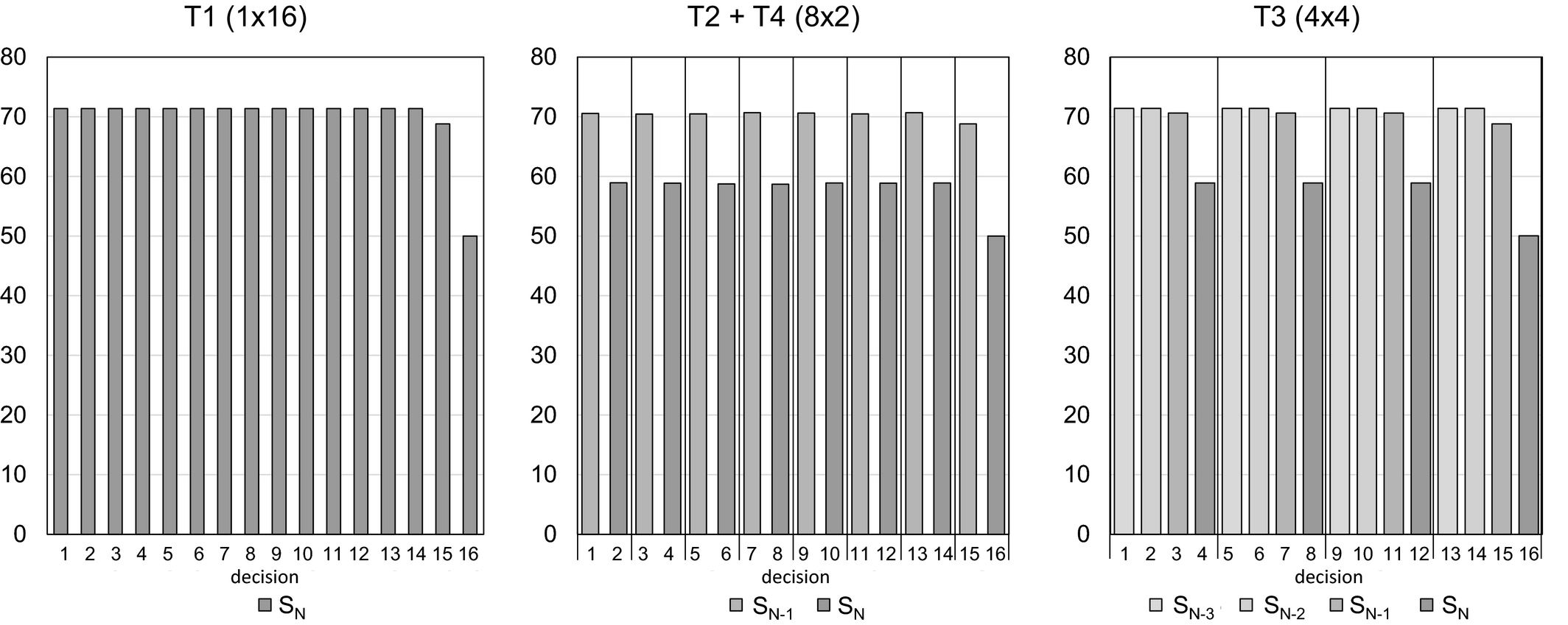
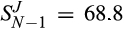
We start with a quick analysis of our baseline treatment (T1). For the first 14 decisions, in which the optimal order‐up‐to level is 71.4, the mean order‐up‐to level is 54.4 (p < 0.001, Wilcoxon signed‐rank test); for decision 15, the mean order‐up‐level is 56.1 (significantly below the optimal level of 68.8, p < 0.001, Wilcoxon signed‐rank test); and for decision 16, the mean order‐up‐to level is 53.2 (not significantly different from the optimal level of 50, p = 0.576, Wilcoxon signed‐rank test). There is no significant difference between rounds 15 and 16 or between the average of rounds 1‐14 and round 15 or 16 (Wilcoxon signed‐rank test, p = 0.22 for subjects’ average order‐up‐to levels in 1–14 vs. 15 and p = 0.52 for 1–14 vs. 16). Figure 7a shows the development over the decisions. Although we are interested mainly in the differences between the treatments, we note that there is a strong pull‐to‐center effect in the 16‐decision newsvendor task. Additionally, we find starting‐inventory effects similar to those in Study 1. Subjects increase the order‐up‐to level by 0.40 for each unit of starting inventory. Table 3 shows the estimation results for the anchoring and starting‐inventory factors (see section 3.2.3 for details of the estimation).

Figure 7

Mean Order‐Up‐To Levels in Treatments 1–4 of Study 2

Table 3

Estimation Results of Behavioral Parameters for Treatments in Study 2

Parameter	T1 (1×16)	T2 (8×2)	T3 (4×4)	T4 (8×2 LIGHT)
Anchoring (θ)	0.785 ***	0.477 ***	0.757 ***	0.485 ***
Anchoring (θ)	(0.112)	(0.132)	(0.076)	(0.112)
Starting inventory ( $β^{'}$ )	0.402 ***	0.106 ***	−0.140	0.176 ***
Starting inventory ( $β^{'}$ )	(0.114)	(0.022)	(0.1032)	(0.036)
Short‐sightedness (α)		0.625 **	0.670 **	0.656 **
Short‐sightedness (α)		(0.179)	(0.151)	(0.178)
N	416	418	403	411
# of clusters	28	29	28	27
LogLike	−1626.82	−1524.45	−1473.39	−1519.48

Note:

Significant values against normative benchmarks (θ = 0, α = 1,

β^{'} = 0

) in bold, standard errors of estimates in parentheses. ***:p < 0.01, **:p < 0.05, *: p < 0.1.

We now analyze the effect of the budget cycle frame for T2. Comparing Figure 7a and b visualizes our first observation: Figure 7b shows a clear cyclic order‐up‐to‐level pattern for the two‐period budget cycle. The order‐up‐to level is significantly lower in the second decisions of each year, with a mean order‐up‐to level of 53.4 (dark‐gray bars in Figure 7b) compared to the first decisions (mean = 60.4, light‐gray bars, p < 0.001, Wilcoxon signed‐rank test). This also holds for each individual year (p = 0.0697 for year 3, p = 0.051 for year 5, and p ≤ 0.001 for all other years).

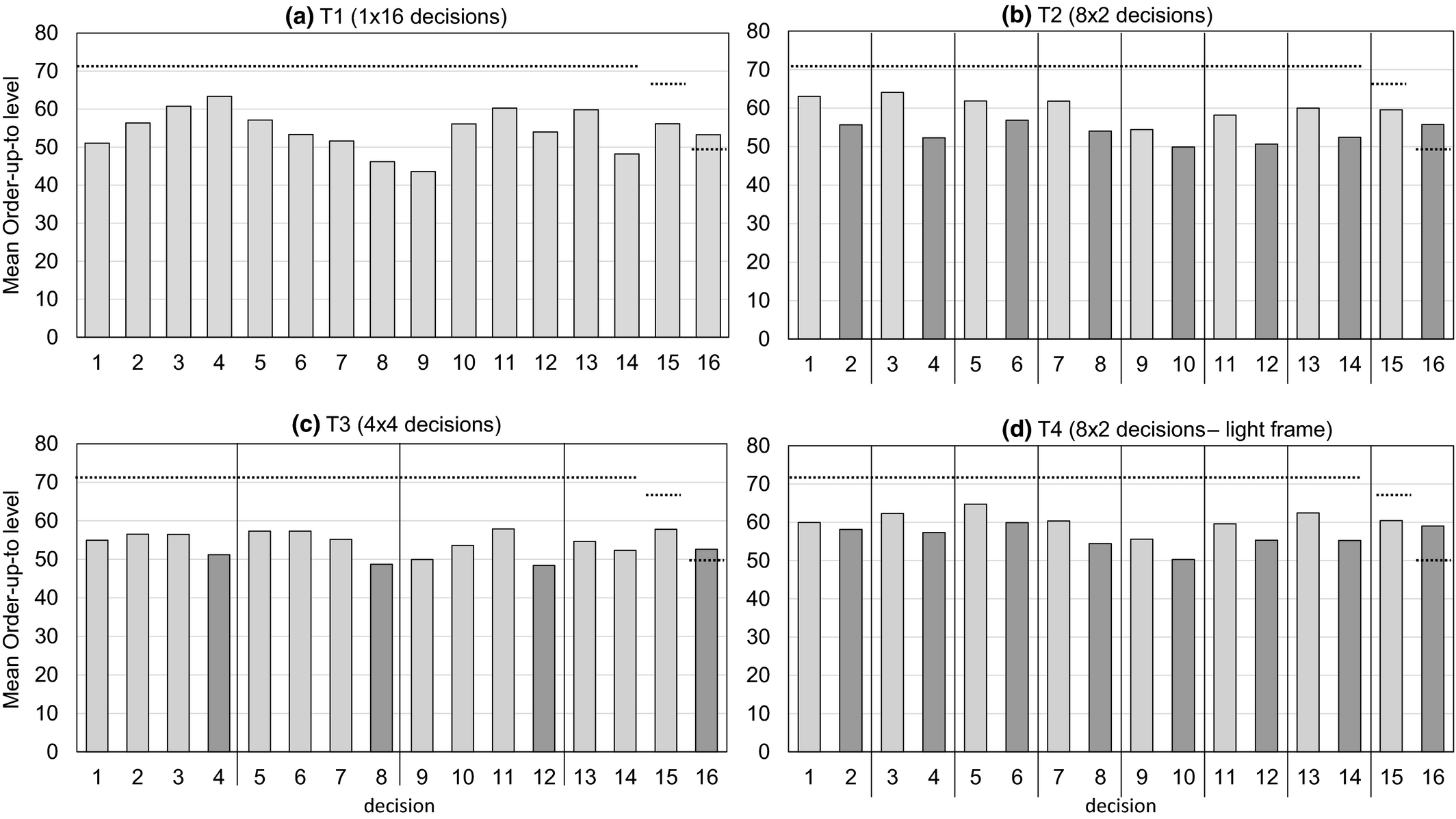
Figure 8a compares the average order‐up‐to level of the first decisions per year for the first seven years with the second decisions of these years (in those years, the normative prediction was 71.4 for all decisions). For these years, the first decisions were also significantly higher than the second decisions (60.5 vs. 53.1, p < 0.001, Wilcoxon signed‐rank test). Note that for decisions 15 and 16 in year 8, there is a normative decline in the order‐up‐to level due to the end‐of‐horizon effect. For the 16‐decision case (T1), there is no significant difference between the corresponding (even and odd) periods. This shows that the narrow frame on two decisions per year leads to short‐sighted decisions. We note again that this is not due to any financial discounting (as in real‐world settings) but due only to the narrow focus.

Figure 8

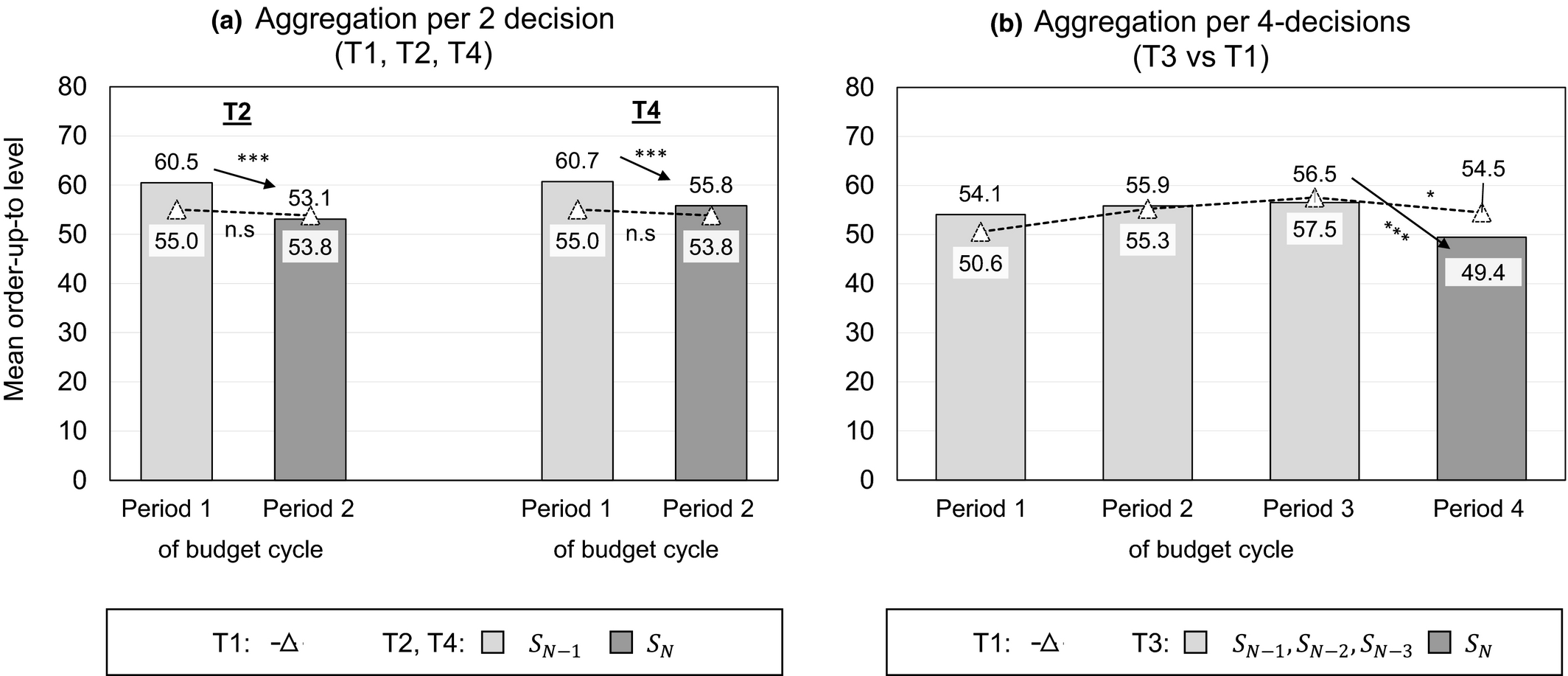
Aggregated Orders for Treatments 1–4 of Study 2

Supporting this argument, Figures 7c and 8b show the order‐up‐to levels for Treatment T3, with four years with four decisions each. Figure 8b shows the significant drop of the order‐up‐to levels in the fourth decision per year (aggregated over the first three years) from 56.5 to 49.4 (p ≤ 0.001). Compared to T2, there is no drop for the second decisions. Figure 7c also visualizes that the cyclic pattern (the drop at the end of the year) is observable in each year (every four decisions in T3). These results support our behavioral short‐sightedness model.

Analyzing the alternative narrow frame in T4, we find qualitatively similar results between the two 8×2 treatments (compare Figure 7b and d). The mean order‐up‐to levels are again significantly lower for the second decisions of a year compared to the first decisions in a year in T4 (60.7 vs. 55.8, p ≤ 0.001, Wilcoxon signed‐rank test, see Figure 8a). Comparing T2 and T4, we find no significant difference between order‐up‐to levels in the first decisions in a year (two‐sample Wilcoxon rank‐sum test of subjects’ average order‐up‐to level between treatments (

N_{T 2} = 29

N_{T 4} = 27

), 60.5 vs. 60.7, p = 0.961), the second decisions (53.1 vs. 55.8, p = 0.496) or the reduction of order‐up‐to levels from first to second decisions (−7.4 vs. −4.9, p = 0.248). We conclude that the effect is robust and not simply based on our strong frame.

A second obvious observation is that order‐up‐to levels are rather low, even in the first decisions. They are significantly below the rational order‐up‐to level (of 71.4) for the first 14 decisions for all of the treatments (p < 0.001, Wilcoxon signed‐rank test). This observation is in line with previously observed mean anchoring. In the previous experiment and in the last decision, the optimal order‐up‐to level equaled mean demand. Therefore, potential mean anchoring did not bias subjects’ decisions there. For the first 15 decisions in this experiment, the optimal order‐up‐to levels are above mean demand. Therefore, mean anchoring pulls order‐up‐to levels towards 50, which may explain the observed differences from optimum, at least for the first decisions per year. Note that mean anchoring cannot explain the cyclic pattern in the order quantities: optimal order‐up‐to levels are the same for

S_{N}

and

S_{N - 1}

in the first seven years; therefore, mean anchoring leads to similar order‐up‐to levels throughout the first 14 decisions (independent of the frame).

A third observation is that the mean order‐up‐to level is not (significantly) above optimum for the very last decision. However, there is a straightforward reason for this: the demand realization in the second last period was very low (

d_{15} = 6

). This resulted in a very high starting inventory for decision 16. On average, the starting inventory was 53.59, which was already above the optimal order‐up‐to level of 50. In that decision, only 9 out of 29 subjects placed an order quantity > 0. This shows that the actual targeted order‐up‐to level is probably below the observed 55.8. Such effect can occur if the targeted order‐up‐to levels decrease over time/decisions and demand realizations are very low.

Combining these factors, we now estimate the behavioral parameters and the effect of these factors.

Estimating Behavioral Parameters

To estimate the behavioral model, we consider three behavioral parameters: the anchor factor θ, the starting‐inventory factor β, and the short‐sightedness factor α. Anchoring on mean demand is classically modeled using the anchor factor θ: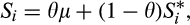

S_{i} = θ μ + (1 - θ) S_{i}^{*},

where

S_{i}^{*}

is the optimal order‐up‐to level for period i. From a normative perspective, we expect no anchoring and therefore θ = 0.

We discussed the starting‐inventory effect in Study 1 in the single‐period model. For the multiperiod model, we use a simple estimation approach: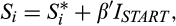

S_{i} = S_{i}^{*} + β^{'} I_{START},

where

β^{'}

represents the fraction of starting inventory that subjects do not deduct from their targeted order‐up‐to level when determining the order quantity (i.e., their starting inventory over‐weighting, see also Equation 7). From a normative perspective, we expect no starting‐inventory effect and therefore

β^{'} = 0

To test the short‐sightedness effect, we first have to analyze how α affects the order‐up‐to levels over the 16 decisions. We denote the number of decisions within a budget cycle as N (the number of budget cycles is denoted as J). As described in section 2.3, there is no closed‐form solution for the behavioral order‐up‐to level

S_{t}^{α}

. To enable an effective estimation, we need to find a closed‐form approximation for

S_{t}^{α}

. To do so, we analyze the numerical results in more detail. Recall Figure 3 and the effect of α on the order‐up‐to levels. Certain observations are important for the further analysis:

The order‐up‐to levels in the last budget cycle (J) are equivalent to the N‐period model (

S_{N}^{J} = S^{*} = 50

and

S_{N - 1}^{J} = 68.8

There is a cyclic pattern for the earlier budget cycles (j < J) with

S_{N - 1} \geq S_{N} \geq S^{*}

(for α ≤ 1).

S_{N}

is the same across earlier budget cycles (j < J) but larger than in the last budget cycle (

S_{N}^{j = 1} = S_{N}^{j = 2} = \dots = S_{N}^{J - 1} \geq S_{N}^{J} = S^{*} = 50

Equivalent relations hold for the comparisons of the second last decisions

S_{N - 1}

between budget cycles.

Earlier decisions in the budget cycles (

S_{N - 2}, S_{N - 3}

) are the same within and across all budget cycles. Additionally, they are not affected by short‐sightedness. In our setting,

S_{N - 2} = S_{N - 3} = 71.4

Based on these observations, we optimize the order‐up‐to level for the two last decisions (

S_{N}, S_{N - 1}

) within earlier budget cycles (j < J) for different α numerically. The results are shown in Figure 9. We observe that the order‐up‐to level decreases for decreasing α (i.e., increasing short‐sightedness). In the extreme case of α = 0, order‐up‐to levels equal those of the two‐period model (

S_{N - 1} = 68.8

for the second last decisions and

S_{N} = S^{*} = 50

for the last decisions in a budget cycle). For rational decision makers (α = 1), the order‐up‐to levels are the same for both decisions (i.e.,

S_{N - 1} = S_{N} = 71.4

for our setting).

Figure 9

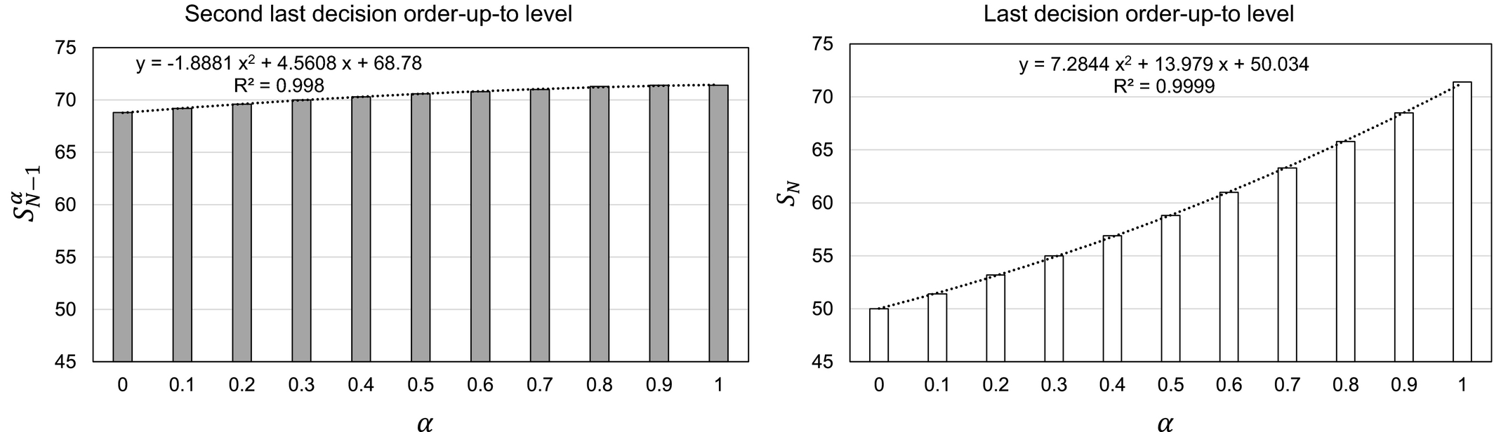
Increasing Factor of Order‐Up‐To Level in the Years before the Last Year (j < J) for Different Levels of Short‐Sightedness

For budget cycles with more than two periods (e.g., N = 4), the order‐up‐to levels for the third last and earlier periods (

S_{N - 2}, S_{N - 3}, \dots

) are not effected by α (see Figure 3). To make the following estimations trackable, we use polynomial approximations of the relationships for (

S_{N}^{α}, S_{N - 1}^{α}

), as shown in Figure 9. The graphs show that a polynomial provides a very good approximation of the relevant range (0 ≤ α ≤ 1) for the short‐sighted order‐up‐to level:

{\tilde{S}}_{N - 1}^{α} = - 1.8881 α^{2} + 4.5608 α + 68.78,

{\tilde{S}}_{N}^{α} = 7.2844 α^{2} + 13.979 α + 50.034 .

Combining the three behavioral factors, the expected behavioral order‐up‐to level (

\bar{S}

) for any period is

\bar{S} = θ μ + (1 - θ) (S_{t}^{α} + β^{'} I_{START}),

with the optimal behavioral order‐up‐to level depending on the period.

For the treatments with two decisions per budget cycle (T2 and T4):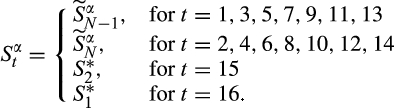

S_{t}^{α} = \{\begin{matrix} {\tilde{S}}_{N - 1}^{α}, & for t = 1, 3, 5, 7, 9, 11, 13 \\ {\tilde{S}}_{N}^{α}, & for t = 2, 4, 6, 8, 10, 12, 14 \\ S_{2}^{*}, & for t = 15 \\ S_{1}^{*} & for t = 16 . \end{matrix}

For treatments with four decisions per budget cycle (T3), the optimal order‐up‐to level for the decision

S_{N - 2}

and

S_{N - 3}

is equal to 71.4 (see Figure 6). This results in the following equation:

S_{t}^{α} = \{\begin{matrix} 71.4, & for t = 1, 2, 5, 6, 9, 10, 13, 14 \\ {\tilde{S}}_{N - 1}^{α}, & for t = 3, 7, 11 \\ {\tilde{S}}_{N}^{α}, & for t = 4, 8, 12 \\ S_{2}^{*}, & for t = 15 \\ S_{1}^{*} & for t = 16 . \end{matrix}

To estimate the effects for our experimental data, we use a nonlinear random‐coefficient model, clustering on subject level. We consider only decisions in which subjects actually placed an order (with a positive order quantity), because for the other decisions, we cannot precisely determine the targeted order‐up‐to level. Table 3 shows the results of our estimation for the different treatments. We find significant and strong effects for all three behavioral factors in all the treatments.⁴

Anchoring. First, subjects anchor on mean demand when deciding on the order‐up‐to level with a weight on the mean demand (θ). Anchoring is strongest in T1 (0.785) and smallest in T2 (0.477). This is unsurprising if we consider that T1 consists of a task in which subjects have 16 decisions on one screen. In T3, there are 4 decisions “at once” and in T2, only two decisions. T4 lies in‐between, because subjects have 16 decisions on the screen but focus instead on the budget cycle with two decisions. Therefore, we expect the task in T1 to be perceived as more complex, leading to a higher degree of anchoring.

Starting inventory. Second, subjects do not fully account for starting inventory but decrease their order‐up‐to level only by

1 - β^{'} = 59.8 %

of the starting inventory in T1. This estimate is bigger in T1 than in the other treatments. Whereas subjects rationally account for starting inventory in T3 (the estimate is not significantly different from 0), they slightly over‐order (by 10.6% and 17.6%) in treatments T2 and T4.

Short‐sightedness. Finally, subjects exhibit short‐sightedness and do not fully account for the effects on the cash flows in the following budget cycles for treatments T2‐T4. The estimates of the short‐sightedness factor (α) are significantly smaller than the normative value of 1 for T2 (α = 0.625, p = 0.018). The light frame in T4 weakens that effect slightly (α = 0.656), but it remains significantly smaller than 1 (p = 0.027). This shows that even under the milder frame in T4, subjects are narrow bracketing and do not account correctly for the future periods, which is in line with the prediction of our behavioral model (Corollary 1). In T3 (with four decisions per year), short‐sightedness is decreased even further (α = 0.670) but remains significantly below 1 (p = 0.014). We note that the full models shown in Table 3 perform significantly better than partial models with fewer parameters (see tables 4–6 in the Appendix for the full comparison).

Summarizing the findings of our experiments, we find non‐expected‐profit‐maximizing ordering behavior. Order‐up‐to levels differ significantly from the optimum for most of the periods. The differences in relation to normative theory can be attributed to three different factors. First, we observe anchoring on mean demand. Although this effect has been observed in previous studies, it is noteworthy that the size of the effect is rather high in our setting. Other studies have reported values between 0.20 and 0.79 in the single‐period newsvendor setting (Becker‐Peth and Thonemann 2018). This rather high value may be driven by the higher complexity in our setting. Higher complexity of decision tasks increases the use of decision heuristics, and a multiperiod decision setting is naturally more complex than a single‐period setting.

Additionally, we observe that decision makers do not fully account for starting inventory. Subjects do not order up to the same inventory level when facing different starting inventories (both with exogenous starting inventory and endogenous starting inventory resulting from previous decisions). This is an interesting finding that has not been explicitly reported in previous studies.

The most interesting finding is that subjects are very short‐sighted and do not properly consider the long‐term effect of their decision. In our multiperiod setting, subjects’ ordering is similar to that of the single‐year setting, and they do not order enough units, especially in the last periods of the year. This cyclic pattern relates to an under‐weighting of future years and periods (

α_{T 2} = 0.496

and

α_{T 4} = 0.558

instead of 1). Generally, loss aversion would reduce the order‐up‐to levels similarly between periods (mixing with mean anchoring in our setting); therefore, loss aversion cannot explain this pattern. We observe this effect even in a setting where there are no rational reasons for decreasing the weight of later decisions, e.g., discounting later payments due to interest rates. This effect has not previously been reported in inventory settings.

Conclusion

In this study, we analyze inventory decisions in multiperiod settings under a cash flow incentive. We focus on the setting in which decision makers make multiple decisions over time with inventory carryover between decisions. Our paper offers two main contributions.

First, we find that starting inventory is not fully considered in the ordering decisions of human decision makers. Interestingly, starting inventory has a significant effect on the order‐up‐to level. Although optimal order‐up‐to levels are the same, higher starting inventory leads to higher actual order‐up‐to levels (our estimates indicate an increase of approximately 30% of the starting inventory). One explanation for this may be an under‐weighting of existing inventory comparable to the under‐weighting of pipeline inventory in the beer game (Croson and Donohue 2006, Sterman 1989). In our experiments, human decision makers order products even when the starting inventory is above the optimal order‐up‐to level. This may also indicate an action bias whereby human decision makers place an order despite not needing to order any goods (e.g., Bar‐El et al. 2007). This effect suggests that it is important to explicitly test the difference between a setting with order‐up‐to levels as a decision variable and a setting with order quantities, and we leave this for future research.

Second, we review the impact of budget cycles in a multiperiod setting. First, we (analytically) show that a finite incentive system, e.g., due to job rotation or fixed‐term contracts, leads to a decrease of order‐up‐to levels towards the end of the incentive system. At the beginning of the time horizon, order‐up‐to levels are constantly on a higher level compared to the end period. The order‐up‐to levels decrease in the last two periods of the incentive horizon. Second, we show that the short‐sightedness of decision makers (e.g., a focus on a budget cycle) has a detrimental effect if budget cycles are used for intermediate incentive payments. Decision makers decrease the order‐up‐to level towards the end of each budget year and do not account for spillovers into future budget cycles. This leads to a cyclic ordering pattern over the budget cycles. Conducting lab experiments, we find evidence that subjects are short‐sighted, focusing on the budget year even in settings in which it is not rational to discount future periods. Testing different lengths of budget cycles and different frames, we find a significant decrease of order‐up‐to levels at the end of the budget cycles even in early periods of the incentive horizon (where there should not be a decrease). This ordering pattern is in line with narrow bracketing, which is known to be relevant in other contexts, e.g., financial decision‐making. Focusing too much on the actual budget cycle, decision makers under‐weight the impact of the decision on future budget cycles. In the extreme case, decision makers may act as if the incentive horizon ends after the current budget cycle, reducing the order‐up‐to levels to single‐period levels at the end of the budget cycle.

Narrow bracketing is usually described as having a negative impact on overall performance (because subjects ignore important effects). However, our experiments show an interesting behavioral effect: narrowing the frame can also improve the performance of decision makers. To demonstrate this phenomenon, we calculated the expected profits for the different treatments for the observed ordering patterns.⁵ We find that expected profits are lowest for the 1×16 Treatment (T1) and highest for the 8×2 treatment (T4) (the difference is weakly significant, p = 0.064). Facing all 16 decisions on one screen, subjects exhibit a stronger pull‐to‐center effect, because the perceived complexity may be higher. Moreover, the variance of the order‐up‐to levels is higher in T1 than in T4 (320 in T1 vs. 240 in T4 and vs. only 159 in T3). Focusing on the current budget cycle, decision makers can solve the task more easily but suffer from the narrow structural frame, leading to an overall improvement for our setting. Analyzing this, there may be an optimal frame that balances the necessary focus and the long‐term horizon. This is an interesting topic which could be addressed in future research.

This also raises the question of whether and how much the problem should be simplified to obtain the best performance. Simplifying the problem leads to worse normative solutions, but human decision makers may be able to find the best solution for this task. This could lead to better overall performances than humans trying (failing) to solve the complex problem and ending up with a worse solution.

In our experimental study, the implemented budget cycles had no effect on normative decision‐making. There was no incremental incentive on lower year‐end inventories (all inventories were accounted), no real time lag between payments (all payments were done at the end of the session), and no additional benefits for reduced final inventories (e.g. signaling efficiency to the stock market). Such factors are likely to additionally affect real‐world decision makers and lead to an even stronger end‐of‐budget‐cycle effect. However, our experiments show that in addition to these factors, the design of incentives and decision‐support tools can have a significant effect. Our experimental design relates to the question of how to design decision‐support tools, because they may also induce such a narrow frame.

These observations have important implications in terms of our contribution to the emerging field of research on the inverse hockey‐stick effect of inventories. Empirical research (Hoberg et al. 2017, Lai and Xiao 2017) has shown that inventory levels decrease significantly toward the end of the fiscal year. Our paper identifies additional factors that may cause such an effect. Decreased order‐up‐to levels directly correspond to reduced expected ending inventories (given constant demand distributions). This means that short‐sighted decision makers intentionally decrease the inventory level towards the end of their individual planning horizons. This is the case for a setting in which no discounting of future returns applies. However, in reality, managers may very well discount future bonus payments, especially if it is uncertain that they will keep their position and responsibilities in the future. Accordingly, short‐sightedness and myopic behavior may apply more strongly in real‐world situations than in our stylized laboratory setting.

These results have implications for future research in behavioral operations management. Previous studies have focused on settings without inventory carryover and no starting inventory. In such settings, order‐up‐to levels are identical to order quantities. However, our results show that both inventory carryover and starting inventory drive the complexity of decisions and affect the ordering behavior of human decision makers. Further, future research could review the cyclic ordering pattern in more detail. In our analysis, we found significant differences between the ordering decisions in the two periods of the budget cycle. However, in real life, there are likely more than two periods and two order decisions in a budget cycle (e.g., many retailers can place orders every day). For accounting purposes, many firms regard performance metrics as incentives that are gathered on a quarterly or monthly basis. Accordingly, it would be interesting for future research to investigate how inventory managers react in settings with more than two periods. We expect that the cyclic pattern would be more pronounced with higher reductions towards the end of the budget cycle but also initial peaks at the start of the budget cycle. However, we leave this analysis to future research.

Our research also provides managerial insights. We find that short‐sighted human behavior leads to higher order and inventory variability. This may cause problems within the supply chain, such as the bullwhip effect. In the theoretical case of an infinite planning horizon, the order‐up‐to levels are also constant. However, incentives in real‐world settings cannot be infinite. Additionally, human decision makers heavily discount future income, which leads to short‐sighted decision‐making. In this study, we assumed the same demand distributions for both periods. However, demand in reality often fluctuates throughout the planning horizon. Seasonal demand can be particularly high on certain days of the week or in certain months of the year. Inventory planners need to manage inventories accordingly and dynamically adjust them throughout the planning horizon. It is important for future research to shed light on the behavioral aspects of changing demand.

Footnotes

Proofs

Additional Analyses

1

In reality, the bonus may also be based on the inventory position at the end of the year. In fact, such an incentive will even increase the effect we observe, a phenomenon we discuss at the end of the paper.

2

For completeness, we note that we also conducted an additional treatment with a different incentive system (Accounting Profit). The results are comparable to the treatment here, and we exclude that incentive system from the paper to improve readability.

3

The subjects additionally played eight single‐period decisions without starting inventory upfront to become familiar with the setting, but for the sake of readability, we exclude the results from the paper.

4

As a robustness check, we estimated the parameters when including zero orders. The results, which exhibit only negligible changes, are included in table in the Appendix. For these cases (where starting inventory is rather high), we overestimate the effect of starting inventory, because the order‐up‐to level is an upper bound for the targeted value. Additionally, we underestimate the short‐sightedness effect, because these cases occur more often in the periods where you aim at lower order‐up‐to levels. However, the factors are still significantly different from 1.

5

We simulated 1,000,000 samples of 16 demand realizations and calculated the profits for the subjects’ order‐up‐to levels observed in the lab.

References

Abdellaoui

Bleichrodt

Paraschiv

. 2007. Loss aversion under prospect theory: A parameter‐free measurement. Management Sci. 53(10): 1659–1674.

Arrow

Harris

Marschak

. 1951. Optimal inventory policy. Econometrica 19(3): 250–272.

Bar‐El

Azar

O. H.

Ritov

Keidar‐Levin

Schein

. 2007. Action bias among elite soccer goalkeepers: The case of penalty kicks. J. Econ. Psychol. 28(5): 606–621.

Becker‐Peth

Thonemann

. 2018. Behavioral inventory decisions: The newsvendor and other inventory settings. Donohue

Katok

Leider

, eds. The Handbook of Behavioral Operations, chap. 11. Wiley, Hoboken, NJ, 393–432.

Becker‐Peth

Katok

Thonemann

. 2013. Designing buyback contracts for irrational but predictable newsvendors. Management Sci. 59(8): 1800–1816.

Becker‐Peth

Thonemann

U. W.

Gully

. 2018. A note on the risk aversion of informed newsvendors. J. Oper. Res. Soc. 69(7): 1135–1145.

Benartzi

Thaler

R. H.

. 1995. Myopic loss aversion and the equity premium puzzle. Q. J. Econ. 110(1): 73–92.

Bendoly

Croson

Goncalves

Schultz

. 2010. Bodies of knowledge for research in behavioral operations. Prod. Oper. Manag. 19(4): 434–452.

Bharadwaj

Gruen

T. W.

Corsten

D. S.

. 2002. Retail out of stocks: A worldwide examination of extent, causes, and consumer responses.

10.

Bolton

Katok

. 2008. Learning by doing in the newsvendor problem: A laboratory investigation of the role of experience and feedback. Manuf. Serv. Oper. Manag. 10(3): 519–538.

11.

Bolton

Ockenfels

Thonemann

. 2012. Managers and students as newsvendors. Management Sci. 58(12): 2225–2233.

12.

Boudreau

Hopp

McClain

J. O.

Thomas

L. J.

. 2003. On the interface between operations and human resources management. Manuf. Serv. Oper. Manag. 5(3): 179–202.

13.

Brealey

Myers

S. C.

Allen

. 2006. Corporate Finance. eight edition. McGraw‐Hill, New York, NY. 84(143) 244–272.

14.

Croson

Donohue

. 2006. Behavioral causes of the bullwhip effect and the observed value of inventory information. Management Sci. 52(3): 323–336.

15.

Croson

Donohue

Katok

Sterman

. 2014. Order stability in supply chains: Coordination risk and the role of coordination stock. Prod. Oper. Manag. 23(2): 176–196.

16.

Dong

Rudi

. 2004. Who benefits from transshipment? Exogenous vs. endogenous wholesale prices. Management Sci. 50(5): 645–657.

17.

Eeckhoudt

Gollier

Schlesinger

. 1995. The risk‐averse (and prudent) newsboy. Management Sci. 41(5): 786–794.

18.

Eroglu

Hofer

. 2011. Lean, leaner, too lean? The inventory‐performance link revisited. J. Oper. Manag. 29(4): 356–369.

19.

Federgruen

Zipkin

. 1986. An inventory model with limited production capacity and uncertain demands II. The discounted‐cost criterion. Math. Oper. Res. 11(2): 208–215.

20.

Fischbacher

2007. z‐tree: Zurich toolbox for ready‐made economic experiments. Exp. Econ. 10(2): 171–178.

21.

Gaur

Fisher

M. L.

Raman

. 2005. An econometric analysis of inventory turnover performance in retail services. Management Sci. 51(2): 181–194.

22.

Gino

Pisano

. 2008. Toward a theory of behavioral operations. Manuf. Serv. Oper. Manag. 10(4): 676–691.

23.

Hartwig

Inderfurth

Sadrieh

Voigt

. 2015. Strategic inventory and supply chain behavior. Prod. Oper. Manag. 24(8): 1329–1345.

24.

Hendricks

Singhal

. 2009. Demand‐supply mismatches and stock market reaction: Evidence from excess inventory announcements. Manuf. Serv. Oper. Manag. 11(3): 509–524.

25.

Herrnstein

R. J.

Prelec

. 1992. T. complexity of addiction is mirrored in the many disciplines. Choice Over Time, 331.

26.

Lim

Cui

. 2010. Reference dependence in multilocation newsvendor models: A structural analysis. Management Sci. 56(11): 1891–1910.

27.

Hoberg

Badorf

Lapp

. 2017. The inverse hockey stick effect: An empirical investigation of the fiscal calendar's impact on firm inventories. Int. J. Prod. Res. 55(16): 4601–4624.

28.

Kahneman

Lovallo

. 1993. Timid choices and bold forecasts: A cognitive perspective on risk taking. Management Sci. 39(1): 17–31.

29.

Katok

D. Y.

. 2009. Contracting in supply chains: A laboratory investigation. Management Sci. 55(12): 1953–1968.

30.

Katok

Thomas

D. J.

Davis

. 2008. Inventory service‐level agreements as coordination mechanisms: The effect of review periods. Manuf. Serv. Oper. Manag. 10(4): 609–624.

31.

Kesavan

Mani

. 2013. The relationship between abnormal inventory growth and future earnings for US public retailers. Manuf. Serv. Oper. Manag. 15(1): 6–23.

32.

Kesavan

Gaur

Raman

. 2010. Do inventory and gross margin data improve sales forecasts for US public retailers? Management Sci. 56(9): 1519–1533.

33.

Kremer

Minner

Van Wassenhove

. 2010. Do random errors explain newsvendor behavior? Manuf. Serv. Oper. Manag. 12(4): 673–681.

34.

Kremer

Minner

Van Wassenhove

. 2014. On the preference to avoid ex post inventory errors. Prod. Oper. Manag. 23(5): 773–787.

35.

Lai

R. K.

2008. Is inventory's fiscal year end effect caused by sales timing? A test using a natural experiment from Germany. Harvard Business School Technology and Operations Mgt. Unit Research Paper, Harvard Business School.

36.

Lai

Xiao

. 2017. Supply chain information signaling and capital market. Handbook of Information Exchange in Supply Chain Management. Springer, Berlin, 215–233.

37.

Long

Nasiry

. 2014. Prospect theory explains newsvendor behavior: The role of reference points. Management Sci. 61(12): 3009–3012.

38.

Monga

2012. Unraveling Inventory's Riddle. Available at http://blogs.wsj.com/cfo/2012/04/10/unraveling-inventorysriddle/ (accessed date November 7, 2019).

39.

Porteus

E. L.

1990. Stochastic inventory theory. Stochastic Models, Handbooks in Operations Research and Management Science, Vol. 2, chap. 12. Elsevier, Amsterdam, 605–652.

40.

Rabin

Weizsäcker

. 2009. Narrow bracketing and dominated choices. Am. Econ. Rev. 99(4): 1508–43.

41.

Read

Loewenstein

Rabin

Keren

Laibson

. 1999. Choice bracketing. Elicitation of Preferences. Springer, Dordrecht, 171–202.

42.

Roychowdhury

2006. Earnings management through real activities manipulation. J. Account. Econ. 42(3): 335–370.

43.

Schweitzer

Cachon

. 2000. Decision bias in the newsvendor problem with a known demand distribution: Experimental evidence. Management Sci. 46(3): 404–420.

44.

Simon

1955. A behavioral model of rational choice. Q. J. Econ. 69(1): 99–118.

45.

Sošić

2006. Transshipment of inventories among retailers: Myopic vs. farsighted stability. Management Sci. 52(10): 1493–1508.

46.

Steinker

Hoberg

. 2013. The impact of inventory dynamics on long‐term stock returns–an empirical investigation of US manufacturing companies. J. Oper. Manag. 31(5): 250–261.

47.

Sterman

J. D.

1989. Modeling managerial behavior: Misperceptions of feedback in a dynamic decision making experiment. Management Sci. 35(3): 321–339.

48.

2008. Bounded rationality in newsvendor models. Manuf. Serv. Oper. Manag. 10(4): 566–589.

49.

Thaler

1999. Mental accounting matters. J. Behav. Decis. Mak. 12(3): 183–206.

50.

Thomas

2005. Measuring item fill‐rate performance in a finite horizon. Manuf. Serv. Oper. Manag. 7(1): 74–80.

51.

Tversky

Kahneman

. 1974. Judgment under uncertainty: Heuristics and biases. Science 185(4157): 1124–1131.

52.

Tversky

Kahneman

. 1991. Loss aversion in riskless choice: A reference‐dependent model. Q. J. Econ. 106(4): 1039–1061.

53.

de Véricourt

Jain

Bearden

Filipowicz

. 2013. Sex, risk and the newsvendor. J. Oper. Manag. 31(1‐2): 86–92.

54.

Wang

Webster

. 2009. The loss‐averse newsvendor problem. Omega 37(1): 93–105.

55.

Zipkin

2000. Foundations of Inventory Management. McGraw‐Hill, New York.

56.

Zipkin

2008. Old and new methods for lost‐sales inventory systems. Oper. Res. 56(5): 1256–1263.

Multiperiod Inventory Management with Budget Cycles: Rational and Behavioral Decision‐Making

Abstract

Keywords

Introduction

Decision‐Making

Rational Single‐Period Model

Rational Multiperiod Model

Behavioral (Short‐Sighted) Multiperiod Model

Experimental Design

Study 1: Single‐Period Model with Starting Inventory

Laboratory Design

Experimental Results

Note:

Endogenous Starting Inventory: The Two‐Period Case

Study 2: Multiperiod Case

Laboratory Design

Experimental Results

Note:

Estimating Behavioral Parameters

Conclusion

Footnotes

Proofs

Additional Analyses

1

2

3

4

5

References