Sage Journals: Discover world-class research

Abstract

Activity network analysis is a widely used tool for managing project risk. Traditionally, this type of analysis is used to evaluate task criticality by assuming linear cause‐and‐effect phenomena, where the size of a local failure (e.g., task delay) dictates its possible global impact (e.g., project delay). Motivated by the question of whether activity networks are subject to nonlinear cause‐and‐effect phenomena, a computational framework is developed and applied to real‐world project data to evaluate project systemic risk. Specifically, project systemic risk is viewed as the result of a cascading process which unravels across an activity network, where the failure of a single task can consequently affect its immediate, downstream task(s). As a result, we demonstrate that local failures are capable of triggering failure cascades of intermittent sizes. In turn, a modest local disruption can fuel exceedingly large, systemic failures. In addition, the probability for this to happen is much higher than anticipated. A systematic examination of why this is the case is subsequently performed, with results attributing the emergence of large‐scale failures to topological and temporal features of activity networks. Finally, local mitigation is assessed in terms of containing these failures cascades – results illustrate that this form of mitigation is both ineffective and insufficient. Given the ubiquity of our findings, our work has the potential of deepening our current theoretical understanding on the causal mechanisms responsible for large‐scale project failures.

Keywords

risk management project failure complex networks systemic risk modeling

Introduction

Understanding project susceptibility to failure is a persistent, and increasingly relevant, challenge across operations research (Gunasekaran and Ngai 2012). Research into understanding the cause of project failure broadly follows two distinct, yet complementary, directions. Several studies have approached this challenge by deploying empirical surveys that focus on the sociological factors that contribute to project failure (e.g., the importance of leadership (Turner and Müller 2005), corporate environment (Schmidt et al. 2001) etc.). Yet such endeavors are exposed to a multitude of biases associated with retrospective studies (Tversky and Kahneman 1974, Watts 2014), complicating the integration of their findings to derive causal mechanisms responsible for project failure (Parvan et al. 2015). A second, and potentially more fruitful (Harrison et al. 2007), approach relies on computational methods that focus on modeling various dynamical properties that condition project failure, from risk culture (Ellinas et al. 2017) and rework dynamics (Jalili and Ford 2016) to propagation of delays (Vanhoucke 2013).

Within this second strand of research, delay propagation is arguably one of the most heavily examined aspects that contributes to project failure (Tavares and Wegłarz 1990). A brief historical overview of models that focus on delay propagation – including critical path method and program evaluation and review technique – is included in Appendix S1, section 1.1. The strength of these models largely lies on the assumption of a linear cause‐and‐effect, the implications of which can be understood with the following example: a single task fails, and the size of its failure determines its impact on the overall project i.e. the completion of a critical task is delayed by x days, with the project being subsequently delayed by x days, at worst. This assumption allows a shift of focus from the way in which tasks interact to the nature of the tasks themselves (Browning and Ramasesh 2007), for example, by minimizing the uncertainty in estimated task duration (Herroelen and Leus 2001). Albeit useful, this simplification leaves more complicated scenarios of project failure unresolved.

For instance, let us consider the case of a different class of failure propagation, by replacing “task delay” with “change order.” In this case, a request to change the specifications of a single task can propagate throughout the project in an unconstrained manner (Jarratt et al. 2011). Consequently, and in contrast to the delay propagation example, the overall impact that a single change order can have on the overall project is not determined by the magnitude of that initial change order. To illustrate, Sosa (2014) reports a case where a single change order was responsible of affecting nearly a third of all tasks, although the initial change was itself, unremarkable. Similarly, Terwiesch and Loch (1999) report a case where change order cascades resulted in a 20–40% increase in the overall project cost; similar cases have also been reported by Mihm et al. (2003), and Loch and Terwiesch (1998). These examples demonstrate the susceptibility of projects to nonlinear failures, where an initially modest disruption can be amplified, and eventually affect the overall project in a disproportionate way.

To account for these nonlinear effects, we focus on the general case of cascading failures, where a generic task “failure” can cascade throughout a project's activity network, with the prospect of affecting a substantial portion of the project. In the context of this study, this risk of having cascades of interdependent failure is referred to as project systemic risk.

The Conditions of Project Systemic Risk

Project systemic risk can have a devastating effect to project performance. One of the most dramatic examples is the case of the Piper Alpha oil production platform in Piper Oldfield, North Sea. On July 6, 1988, a rather minor aspect of a maintenance project was to go horribly wrong, resulting to the world's deadliest offshore oil industry disaster. A public enquiry led by Lord Cullen (1990) established the narrative of the incident, where the failure to complete a task (sealing of an open pipe) triggered a domino‐like series of unfortunate, yet seemingly preventable, failures that eventually led to the loss of 167 people and damages worth 3.4 billion USD. The final report made a total of 106 recommendations to ensure a similar line of failures could not be repeated.

Importantly, this failure cascade was deemed to be enabled by a set of extraordinary conditions, such as a defeated structural design and negligent organizational culture (NASA 2013). This is an example of a consistent trend throughout the project management literature, where large‐scale project failures are attributed to extraordinary conditions (Kappelman et al. 2006, Pinto and Mantel 1990). As a result, extraordinary conditions are often assumed to be necessary for a large‐scale failure to occur.

Complexity science offers an alternative view, where large‐scale failures occur for the exact same reason(s) as small ones do, that is, ordinary conditions (Albert et al. 2000, Bak et al. 1987, McAteer et al. 2015). Particularly, it has been argued that despite the unique nature of each failure, common principles are in place (Bak and Paczuski 1995). These principles essentially reside to: (a) the rules that govern dynamical processes, such as the propagation of failure (Bak et al. 1987, Vespignani 2012), and (b) the topological features that enable such processes to materialize in the first place (Albert et al. 2000, Pastor‐Satorras and Vespignani 2001, Rahmandad and Sterman 2008, Williams 2002). Insights into the fragility of critical infrastructure (Buldyrev et al. 2010) and resilience of global supply chains (Kim et al. 2015), the sensitivity of the financial market (Schweitzer et al. 2009) and the persistence of viruses (Vespignani 2012) are some of the hallmarks of the approach. See Appendix S1, section 1.2 for a brief overview of additional work, and Appendix S1, section 1.3 for its relevance to projects.

Our work expresses this alternative view by contextualizing principles from complexity science to the domain of project management. We specifically focus on how task interactions support nonlinear failure mechanisms, in the form of generic failures cascading through a project in a domino‐like fashion. By doing so, we relax the linear cause‐and‐effect assumption. Each domino‐like failure is triggered by a modest disruption – the failure of a single task – and therefore, observing any significant impact on the overall project implies that extraordinary conditions are not necessary for large‐scale, project failures to occur.

Our work makes three core contributions. First, we model large‐scale project failures in the form of domino‐like failures cascading throughout a network. Results of our analysis indicate that projects are exceedingly prone to large‐scale failures, both in terms of their absolute size and probability of occurrence. Assessing these large‐scale failures in a quantifiable way has the potential of deepening our current theoretical understanding on the causal mechanisms responsible for large‐scale project failures, which is currently restrained by two widely held assumptions – that project failure is driven by linear cause‐and‐effect, and that extraordinary conditions are necessary for large‐scale, project failures to occur. Secondly, we systematically explore the cause of increased project susceptibility towards large failure cascades, with certain project features being identified as key enablers. In doing so, we are able to provide actionable insight for controlling damaging effects of these failures cascades. This is in contrast to cases where large‐scale failures are attributed to extraordinary conditions, which tend to be generic in nature, and therefore limiting in terms of actionable insight (Zwikael and Globerson 2006). Thirdly, the ability of local mitigation to contain the propagation of failure cascades is evaluated, with results demonstrating both its ineffective and inefficient nature. As such, we provide quantifiable evidence in support for the complex nature of modern projects, stressing the need to look beyond conventional approaches when dealing with risks associated with these projects (Geraldi et al. 2011, Williams 1999).

Experimental Design

Data

Risk management is a key enabler for successful project delivery, through identification and reduction in project risk levels (Zwikael and Ahn 2011). The majority of risk management practices is performed during the planning phase of a project (Maytorena et al. 2007), where the project plan lies at the core of delivering it (Zwikael and Sadeh 2007). For the reader's reference, Zwikael and Ahn (2011) define the planning phase as “the establishment of a set of directions provided in sufficient detail to inform the project team of exactly what must be done, when it must be done, and what resources to use to produce the expected results of the project successfully”.

Project plans encompass a variety of information related to the planning phase, including activity networks that identify the sequence of tasks that needs to be done, at any given point in time (Vanhoucke 2010). As such, we deploy project plans from 5 construction projects, with 2 plans per project capturing the state of the plan at different points in time (Table 1). Construction projects are regularly deemed to have the highest level of risk among other type of engineering projects (Zwikael and Ahn 2011), and therefore provide an ideal context to explore project systemic risk. More generally, projects composed of technical activities are the backbone of modern organizational activity (Shenhar 2001), further strengthening the relevance of this dataset.

Table 1

Summary of Empirical Dataset and Respective AON Networks

Project type (cost, USD)	Project plan information				AON network
Project type (cost, USD)	Project plan	Project start date	Plan modified after (days)	Expected duration (days)	Node count, N	Edge count, E
Educational Institution ($15,000,000)	#1	10/09/2009	+40	366	935	1,070
Educational Institution ($15,000,000)	#2	10/09/2009	+104	344	1,037	1,198
Commercial Offices ($13,000,000)	#3	15/09/2004	+604	744	833	867
Commercial Offices ($13,000,000)	#4	15/09/2004	+709	734	802	810
Undisclosed (Undisclosed)	#5	04/12/2004	+45	419	753	820
Undisclosed (Undisclosed)	#6	04/12/2004	+115	405	779	850
Medical Institution ($7,000,000)	#7	22/09/2003	+1	596	513	563
Medical Institution ($7,000,000)	#8	22/09/2003	+14	562	514	563
Commercial Offices ($5,000,000)	#9	16/07/2006	+12	549	326	435
Commercial Offices ($5,000,000)	#10	16/07/2006	+122	593	312	369

Notes

Information includes the project start date (Column 2), the point in which the project plan used was produced relative to the project launch (Column 3), and the expected project duration (Column 4)

Formally, each project plan is abstracted using the activity‐on‐the‐node (AON) network notation (Valls and Lino 2001), in the form of a directed graph G = {{N} {E}}, where every node i ∈ N, corresponds to task i and a directed link e _i,j ∈, E, account for the precedence relationship between tasks i and j. A relationship between task i and j further requires that task i must first be completed, for task j to start, that is, task j is, in relation to task i, a downstream task (similarly, task i is, in relation to task j, an upstream task) (Krishnan et al. 1997). As a result, a temporal direction to all possible failures exist, where a failure in task i can only affect downstream tasks – which are scheduled to start once task i is completed – but not upstream tasks, as these tasks have already been completed.

Overview of the Cascade Model

A failure cascade corresponds to the outcome of a cascading process, where node i fails and has the potential to affect its immediate, downstream node(s) j. If node(s) j fails, the process has the potential to continue (i.e., node j is now considered to be node i) and affect additional downstream nodes until the process is brought to a stop. This can happen either because node i has no immediate downstream nodes or because the failure of node i has had no effect to the state of node j.

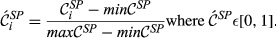
In this context, the state of node i (s _i) is described by one of two possible values – 1 if node i is “affected” (s _i = 1)’ or 0 if “non‐affected” (s _i = 0); this is a well‐established premise when modeling cascading effects in both natural (Kermack and McKendrick 1932) and social sciences (Granovetter 1978). Note the generic nature of the term “affected” which reflects the general nature of these dynamics, since failure can mean very different things, depending on the context of a particular project. For example, “failure” can mean “structural defect” in a construction project, or something much less tangible such as “contaminated” or “compromised” in a cyber‐security project. Every node is also described by a threshold value (θ), which reflects its capacity to function. Therefore, a node with a “non‐affected” state can irreversibly switch to an “affected” state if its own threshold exceeds a given failure threshold (Granovetter 1978). The use of failure thresholds to model cascading effects is widely adopted across a broad range of domains – for additional details see the reviewing work of Pastor‐Satorras et al. (2015) – particularly Section X.A – and Porter and Gleeson (2016).

The impact of node i's failure can be numerically explored by artificially failing it (i.e., switch its state from “non‐affected” to “affected”) and examine its capacity to affect its immediate downstream node(s) j, which are now considered to be stressed. The amount of “stress” node(s) j receives is a function of its exposure to the failure of node i – node(s) j's “sensitivity” – and to node i's ability to convey the effects of its failure – node i's “spreading power.” Following the failure of node i, the new threshold of node j − θ(new)– is a combination of the aforementioned quantities “sensitivity” and “spreading power.” As such, if the new threshold is lower than a given percentage of node j's initial threshold –

θ (initial)

– then node j fails and has the opportunity to fuel the cascade further by affecting its own downstream nodes.

Two fundamentally different mechanisms are in play here – (a) the mechanism responsible for node i switching its state, from “non‐affected” to “affected,” and (b) the mechanism responsible for the spread of the effect of this switch. Mechanism (a) can exist regardless of whether node i is connected to other nodes or not (i.e., a task can fail regardless of whether it links to other upstream or downstream tasks), while mechanism (b) is solely driven by interconnectivity (i.e., failure of a task can only spread if that task is linked to additional downstream tasks). As we focus on the implications of nontrivial interconnectivity, we explicitly focus on the spreading mechanism (b), and therefore introduce the impact of (a) by replicating its effect in an artificial manner (i.e., by artificially failing task i), similar to (Rahmandad and Sterman 2008, Watts 2002). By doing so, we focus on the impact that a single failure can have on the remaining network.

Definition of Cascade Model Components

Quality of Completion

The quality of completion for each task is a function of numerous parameters, one of them being the ability to dispense resources as originally planned (e.g., time, material, labor, equipment, etc.). Therefore, the aim is to minimize the deviation between actual and planned resource expenditure (ideally zero) (PMI 2008). With temporal aspects being the most frequently‐used quantities for project risk management (Zwikael and Sadeh 2007), we will assume that the deviation between time planned (

T_{i}^{plan}

) and actual time spent (

T_{i}^{actual}

) for the delivery of task i is the sole parameter that affects its quality of completion (q _i). In this context, the notion of quality of completion is general enough to apply to a wide range of projects, yet specific enough to capture the all‐important duality between quality and time.

The uncertainty in delivering node i within the planned time can be modeled stochastically by introducing a perturbation term

β_{i}^{pdf}

, reflecting the actual amount of time spent on task i:

T_{i}^{actual} = \{\begin{matrix} T_{i}^{plan} + β_{i}^{pdf}, & if T_{i}^{plan} + β_{i}^{pdf} > 0 \\ 1 & otherwise \end{matrix},

(1)

where

β_{i}^{pdf}

is uniformly drawn at random from a predefined, probability density function (pdf) – in this case

β_{i}^{pdf} \sim N (0, 2) .

Subsequently, by considering the effective time spent, defined as

{\hat{T}}_{l} = \frac{T_{i}^{actual}}{T_{i}^{plan}},

the impact of

T_{i}^{actual} \neq T_{i}^{plan}

on the quality of completion of task i can be explored. The assumption here is that effective, rather than actual, time is the determining factor for achieving the agreed quality of completion, which is in step with standard practice (i.e., numerous constructs are defined based on the same principle, from the general notion of project control to the formulation of performance indices such as the schedule performance index (PMI 2008)).

The nature of the relationship between q _i and

{\hat{T}}_{i}

reflects the cumulative improvement in quality as resource expenditure increases. Equally, it reflects the change in completed quality if this line of resource is perturbed. Hence, let us refer to the relationship between q _i and

{\hat{T}}_{i}

as the resource sensitivity profile (RSP) function. Though the exact shape of the RSP for every task i is not known, it needs to have a number of essential features:

A task will have a quality of 0 unless some resource has been spent;

Quality increases monotonically as the cumulative resource that drives it also increases;

If the task receives exactly its planned resource it will achieve an almost perfect quality of completion. This is because its quality of completion can always increase (even infinitesimally small) if resource expenditure continues to increase;

A task cannot have a quality higher than a maximum of 1.

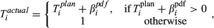
As such, three distinct RSP functions are formulated – linear, sigmoidal and exponential – each defining the sensitivity of particular task archetypes to resource perturbation (Figure 1). A task with a linear RSP is one where change in its quality is directly proportional to the time spent towards its delivery. Such tasks are rather sensitive to resource perturbation, as halving the resource spent will cause a substantial drop in quality. A task with a sigmoidal RSP is one with a shifting behavior. Initially, increasing resource expenditure can substantially increase the resulting quality; beyond a point this behavior shifts to one where increased resource expenditure has a diminished return. Therefore, resource perturbation can have a range of effects, depending on the point at which it is applied. Finally, a task with an exponential RSP is one where change in its quality is disproportionately dependent on the time spent, saturating early at an almost perfect value. Such tasks are robust to resource perturbation, as halving the resource spent will cause a relatively small drop in quality. Relevant mathematical definitions are included in Appendix S1, section 2.

Figure 1

Three Model Resource Sensitivity Profiles (RSP) Functions, Mapping the Relationship between Effective Time Spent (x‐axis) and Quality of Completion (y‐axis) for Task i [Color figure can be viewed at wileyonlinelibrary.com]

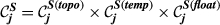
Spreading Power of Node i

The “spreading power” of node i

(C_{i}^{SP})

is a function of both topological and temporal features of the AON network, denoted as

C_{i}^{SP (topo)}

and

C_{i}^{SP (temp)}

, respectively. The core concepts are summarized in Table 2.

Table 2

Core Aspects that Determine the “Spreading Power” of Task i

Spreading Power of task i , $C_{i}^{SP} = C_{i}^{SP (topo)} \times C_{i}^{SP (temp)}$
Topological aspect	$C_{i}^{S P (t o p o)}$ ∝ number of paths between task i and j, weighted by path length
Temporal aspect	$C_{i}^{S P (t e m p)}$ ∝ ratio between duration of task i and project duration

Parameter

C_{i}^{SP (topo)}

considers the position of a task within the AON network by accounting for the effectiveness by which task i can reach, and hence affect, its immediate downstream tasks(s) over all possible paths. In addition, longer paths contribute less to the overall spreading power as they are less likely to be traversed, compared to shorter, more direct paths (Schilling and Phelps 2007). Shifting focus to the temporal aspect,

C_{i}^{SP (temp)}

formalizes the premise that the longer a task is, in terms of T ^actual, the greater its ability to affect its immediate downstream tasks. As an example, consider the AON network in Figure 2a, where task i can affect task l in a direct and indirect way (via task j); in comparison task k can only do so in a direct way (Figure 2b). Therefore,

C_{i}^{SP (topo)}

is higher than

C_{j}^{SP (topo)}

. In a similar spirit,

C_{k}^{SP (temp)}

is higher than

C_{j}^{SP (temp)}

since task k consumes a larger portion of the overall project duration, compared to task j (Figure 2c). Additional details for

C_{i}^{SP (topo)}

and

C_{i}^{SP (temp)}

are included in Appendix S1, section 3.

Figure 2

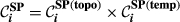
(a) Example Network that Illustrates the Two Aspects Captured Within “Spreading Power”, For Task i and j, in Terms of: (b) Possible Pathways and, (c) Task Duration [Color figure can be viewed at wileyonlinelibrary.com]

The overall “spreading power” of task i is necessarily zero if any of its two constituent aspects is zero. That is, a task with no duration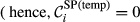

(hence, C_{i}^{SP (temp)} = 0

or no immediate downstream asks

(hence, C_{i}^{SP (topo)} = 0)

can have no spreading power. Therefore, the overall “spreading power” of task i can be defined as:

C_{i}^{SP} = C_{i}^{SP (topo)} \times C_{i}^{SP (temp)} .

(2)

Note that under this formulation, both components have equal weights. Finally, since q(i) ϵ [0,1],

C_{i}^{SP}

is normalized so that both q and

C_{i}^{SP}

(and

C_{j}^{S}

; see Section 3.3.3) are of identical range to ensure the condition set in equation 7 is computed in an unbiased way:

{\overset{´}{C}}_{i}^{SP} = \frac{C_{i}^{SP} - m i n C^{SP}}{m a x C^{SP} - m i n C^{SP}} where {\overset{´}{C}}^{SP} ϵ [0, 1] .

(3)

Sensitivity of Node j

In step with the definition

C_{i}^{SP},

the “sensitivity” of task j

(C_{j}^{S})

to the failure of its immediate upstream task(s) is also a function of the topological and temporal features of the AON network, denoted by

C_{j}^{S (topo)}

and

C_{j}^{S (temp)}

respectively. In addition, the time between two consecutive tasks – the so‐called float – is introduced as an additional temporal component, denoted by

C_{j}^{S (float)}

. Note that the inclusion of an additional temporal component (compared to “spreading power” definition) does not bias the results in any way (see Appendix S1, section 6). The core concepts are summarized in Table 3.

Table 3

Core Aspects that Determine the “Sensitivity” of Task j

Sensitivity of task j , $C_{j}^{S} = C_{j}^{S (t o p o)} \times C_{j}^{S (t e m p)} \times C_{j}^{S (f l o a t)}$
Topological aspect	$C_{j}^{S (topo)} \propto$ number of task(s) i that can affect task j
Temporal aspect	$C_{j}^{S (temp)} \propto$ ratio between project duration and duration of task j
Temporal aspect	$C_{j}^{S (float)} \propto$ float between task i and j

C_{j}^{S (topo)}

considers the number of upstream tasks that directly link to task j, where a higher number implies that there are simply more things that can go wrong and affect the delivery of task j.

C_{j}^{S (temp)}

reasons that a longer task, in terms of T ^actual, is less sensitive to the failure of its immediate upstream task(s), due to an increased capacity to encompass additional work that can mitigate the effect of such failure. Finally,

C_{j}^{S (float)}

considers the impact of float between two consecutive tasks. In the case of a task i failing, the float between task i and j restrains the response time available for mitigation to be deployed. As a result, high float increases the possibility of task j to remain unaffected by the failure of task i, as the available time to respond is high, and vice versa. As an example, consider the AON network in Figure 3a, where the start of task l depends on the completion of task k and j; in comparison the start of j depends only on task i (Figure 3b). Therefore

C_{l}^{S (topo)}

is larger than

C_{j}^{S (topo)}

. In a similar spirit,

C_{l}^{S (temp)}

is larger than

C_{j}^{S (temp)}

since task l consumes a smaller portion of the overall project duration, compared to task j (Figure 3c). Finally, the float between task l and its upstream tasks is larger compared to the float between task j and its upstream tasks, making

C_{j}^{S (float)}

larger than

C_{l}^{S (float)} .

Additional details for

C_{j}^{S (topo)}

C_{j}^{S (temp)}

and

C_{j}^{S (float)}

are included in Appendix S1, section 4.

Figure 3

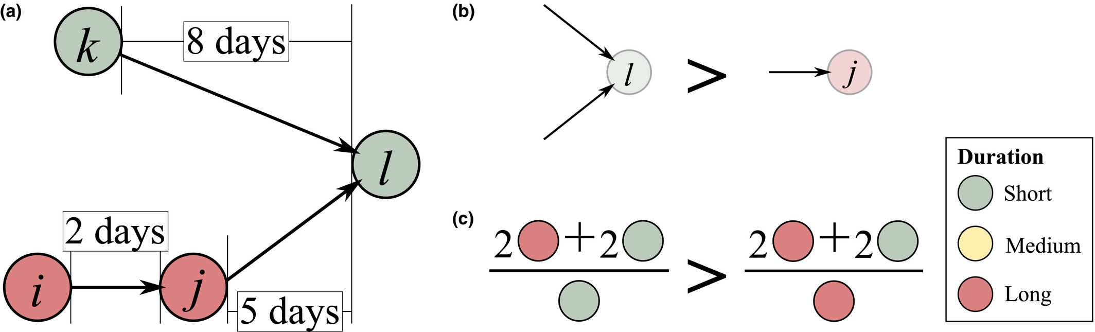
Example Network that Illustrates the Three Aspects Captured Within “Sensitivity”, For Task i and j, in Terms of: (a) Float, (b) Number of Immediate Upstream Tasks, and (c) Task Duration [Color figure can be viewed at wileyonlinelibrary.com]

The overall sensitivity of task j is necessarily zero if any of its three constituent aspects is zero. That is, a task with no immediate upstream tasks, with infinite duration or infinite float can have no sensitivity. In practice, only the first condition can be achieved, the latter two being theoretical, yet practically unattainable, possibilities. This suggests that the only way in which a task can have no sensitivity is to be independent of other tasks. In the context of failure cascades, this is a reasonable assumption: as long as there is a path between task i and j, task j will always be exposed to the failure of task i, albeit to a varying extent (which is controlled by the task's duration and float). Therefore, the overall “sensitivity” of task j can be defined as follows: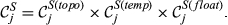

C_{j}^{S} = C_{j}^{S (t o p o)} \times C_{j}^{S (t e m p)} \times C_{j}^{S (f l o a t)} .

(4)

All three components of

C_{j}^{S}

have an equal weight, with

C_{j}^{S}

further being normalized in a similar fashion obtaining

{\overset{´}{C}}_{j}^{S} ϵ [0, 1]

(see equation 3).

Cascade Model Dynamics

Initially, the state of each node is set to “non‐affected.” Subsequently, every task is assigned a RSP function which determines its sensitivity to resource perturbation. For this work, the sigmoidal RSP is assigned to all tasks due to its wide adoption across the PM domain (PMI 2008). The planned duration for each task is subsequently perturbed to derive the actual duration, and from there the effective time spent. Effective time is then used to determine the quality of completion of each task, which serves as the initial failure threshold. In the case of task j, this corresponds to the following: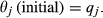

θ_{j} (initial) = q_{j} .

(5)

At this point, the cascading process is initiated by picking task i and artificially failing it by switching its state from “non‐affected” to “affected.” As a result, the state of all of its immediate downstream task(s) j, is reassessed in order to evaluate the effect that the failure of task i has to task(s) j's state. To do so, new thresholds are computed for all task(s) j, based on the “spreading power” and “sensitivity” of task i and j respectively: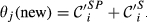

θ_{j} (new) = {C^{'}}_{i}^{SP} + {C^{'}}_{i}^{S} .

(6)

θ_{j} (new)

is greater than a given percentage of

θ_{j} (initial)

, then task j fails and has the opportunity to fuel the cascade further by affecting its own immediate, downstream task(s).

This percentage is controlled by parameter, α, which essentially regulates the magnitude by which

θ_{j} (new)

must exceed

θ_{j} (initial)

for task j to fail – see RHS of equation 7. On one end of the spectrum (α = 0), the failure of task i guarantees the subsequent failure of task j. Hence, the final failure cascade size is the largest possible one, being determined solely by the features of the AON network. Beyond this point

(α > 0)

, the probability for the failure of node i to affect node j reduces, with the final failure cascade size being determined by both network features and the magnitude of parameter α.

In practice, parameter α scales the quality of completion function. Therefore, a higher α value means that a higher quality of completion can be achieved while spending the same amount of effective time; conversely, the same quality can be achieved while spending less effective time. As an example, consider the case where a task is almost halfway towards achieving its specified quality, yet has depleted most of its allocated effective time. To maximize the impact of the remaining effective time, a decision maker can increase the rate by which quality improves (e.g., by assigning additional personnel, deploying more efficient technology, etc.). The effect of such action is essentially equivalent to an increase in α. In the context of failure cascades, varying α corresponds to a localized effort in reducing the likelihood that the failure of task i affects task j by increasing task j's quality of completion. Note that although α is applied uniformly across all tasks, its influence is limited to local, pairwise interactions. In contrast, global mitigation would require an intervention affecting the entirety of nodes (e.g., tailoring particular network features, as specified in Section 3.5).

The majority of cascade models incorporate an absolute failure threshold, either drawn from empirical estimates, for example, (Battiston et al. 2012), or using purely arbitrary values, for example, (Watts 2002). Yet in the context of projects, no absolute value can be considered to be a sensible choice for all types of tasks, due to the potential for large variance to exist across definitive task characteristics (e.g., float can vary across several orders of magnitude (Ellinas et al. 2016b)). As such, a relative failure threshold is introduced through equation 7, where task j switches state if the failure of task i induces a change to task j's threshold, greater than a given size. In other words, the “non‐affected” task j can become “affected” if the failure of task i induces a change in a given size to task j's quality of completion. By doing so, we assume that task j will not necessarily fail on the grounds of poor quality, but rather on its inability to cope with large deviation in its quality of completion. In other words, it is more likely for a poorly completed task to still be delivered, unlocking its downstream tasks, compared to one that has achieved a higher level of quality but has sustained extensive changes.

Finally, Table 4 details the algorithm used to implement the cascade dynamics.

Table 4

Algorithm Detailing the Implementation of the Model Dynamics

Step 1: Model parameterization

1a: Set model parameter: α, α

ϵ

[1,200]

1b: Define a resource sensitivity profile (RSP)

Step 2: Model initialization

2a: Draw task fluctuations

β_{i}^{pdf}

from a specified statistical distribution

2b: Set

q_{i} = R S P [{\hat{T}}_{i}]

for all i

2c: Define initial node states at time t = 0:

s_{i} (0) = \{\begin{matrix} 1, & if i = = k \\ 0, & otherwise \end{matrix}

Step 3: Model dynamics

3a: Iterate simulated time t = 1, 2, …, until no more change happens:

– For all “affected” nodes i (i.e., nodes where s _i = = 1):

– For all immediate downstream nodes j of node i:

s_{j} (t) = \{\begin{matrix} 1, & if θ_{j} (new) \geq \frac{α}{100} \times θ_{j} (initial) \\ s_{j} (t - 1), & otherwise \end{matrix}

(7)

Step 4: Model outcome

4a: The percentage of affected nodes:

\frac{1}{n} \sum_{i = 1}^{n} s_{i}

Features that Control Project Susceptibility

AON networks are characterized by significant levels of heterogeneity (e.g., a few tasks are substantially more connected than the average task) and nontrivial patterns (e.g., longer tasks are more likely to be followed by shorter tasks) (Ellinas et al. 2016b). At the same time, AON networks are constructed around a task order restriction, where task i can unlock task j only if task i is completed first. Understanding how these features impact the cascading process is an important perquisite for reducing the overall susceptibility of AON networks to large‐scale failure cascades. To do so, variants of the original AON networks are constructed, which selectively preserve a number of key features while eliminating others. These network variants are referred to as null models. Therefore, any difference between the behavior of a particular null model and the original AON network can be attributed to the feature(s) absent from that null model.

In general, each null model is generated through normalizing or reshuffling certain aspects of the original AON network, in effect destroying the heterogeneity and/or correlation that determines a given network feature – see Table 5. Every network feature is classified in terms of its nature – topological or temporal – and examined independently from the rest. This focused approach is adopted for two main reasons: (a) to avoid possible confounding effects that can arise by jointly examining the influence of topological and temporal features, and (b) decision makers have different capacities to alter features under these two classes.

Table 5

Null Models of the Original AON Network, Where Specific Network Features are Preserved and/or Destroyed

Activity network	Topology			Temporal
Activity network	Topological correlations	Task order	Heterogeneity	Duration heterogeneity	Temporal correlations
Original	✓	✓	✓	✓	✓
Null model 1	Destroyed	✓	✓	✓	✓
Null model 2	Destroyed	Destroyed	✓	✓	✓
Null model 3	Destroyed	✓	Destroyed	✓	✓
Null model 4	✓	✓	✓	Destroyed	✓
Null model 5	✓	✓	✓	✓	Destroyed

In detail, Null Model 1 rewires the entirety of connections whilst preserving the original in/out degree of each task; in addition, the order of all tasks is preserved. Null Model 2 repeats the same procedure while ignoring the task order restriction, that is, a particular task sequence can be reshuffled. Null Model 3 assigns a new in/out degree for each task, based on an appropriate Normal distribution, while preserving their order. By doing so, the original degree heterogeneity of the AON network is destroyed. In addition, all nontrivial topological correlations are destroyed. Null Model 4 and 5 focus on the temporal features of the network, with Null Model 4 applying the same approach to Null Model 3 to the task duration. Naturally, all topological aspects are preserved. Finally, Null Model 5 reshuffles the duration of each task – again all topological aspects are preserved. Note that due to the nondeterministic network configuration that results from every null model, an ensemble of 30 independent networks is used for the analysis.

To highlight the effect of applying each null model, consider the simple AON network in Figure 4a. In this case, node color reflects the duration of each task, whilst the node label reflects the order in which each task is delivered. In relation to the features noted in Table 5, the following observations can be made: (i) topological correlations exist (e.g., high‐degree nodes tend to connect with low‐degree nodes); (ii) tasks are delivered in a particular order (e.g., from task 1 to 2 to 3 etc.); (iii) connectivity is heterogeneous in nature (e.g., task 1 is disproportionately connected compared to the rest tasks); (iv) task duration is heterogeneously spread (e.g., task 1 consumes disproportionately more time than the rest) and (v) temporal correlations exists (e.g., the high duration task is preceded by medium duration tasks, followed by short duration tasks). In comparison, Null Model 1 preserves all aspects but (i), since task 2 is now connected with task 7 instead of task 6, which possesses 2 connections instead of 1. Similarly, Null Model 2 eliminates (i) and (ii) by allowing task 3 to precede task 2. Null Model 3 eliminates (i) and (iii), where every task has a similar number of connections. Null Model 4 and 5 shift focus to the temporal aspects, with Null Model 4 smoothening the difference in task duration across all tasks, while Null Model 5 eliminates any temporal correlations that may have existed in the original network (e.g., the correlation between medium and long duration task is present in the original, yet absent from Null Model 5). It is worth noting that the total number of tasks and connections in every null model realization is preserved.

Figure 4

Example of How Network Features can be Selectively Removed in Order to Identify their Effect with Respect to their Susceptibility to Failure Cascade. AON Network (a) Serves as the Original Case, with (b)–(f) Providing Examples of Null Models 1–5 [Color figure can be viewed at wileyonlinelibrary.com]

Note: Node colour reflect the duration of each task; node label reflects the order of task completion. Dotted and red connections correspond to removed and newly‐introduced links, respectively.

Results

Evaluating Project Susceptibility to Systemic Failures

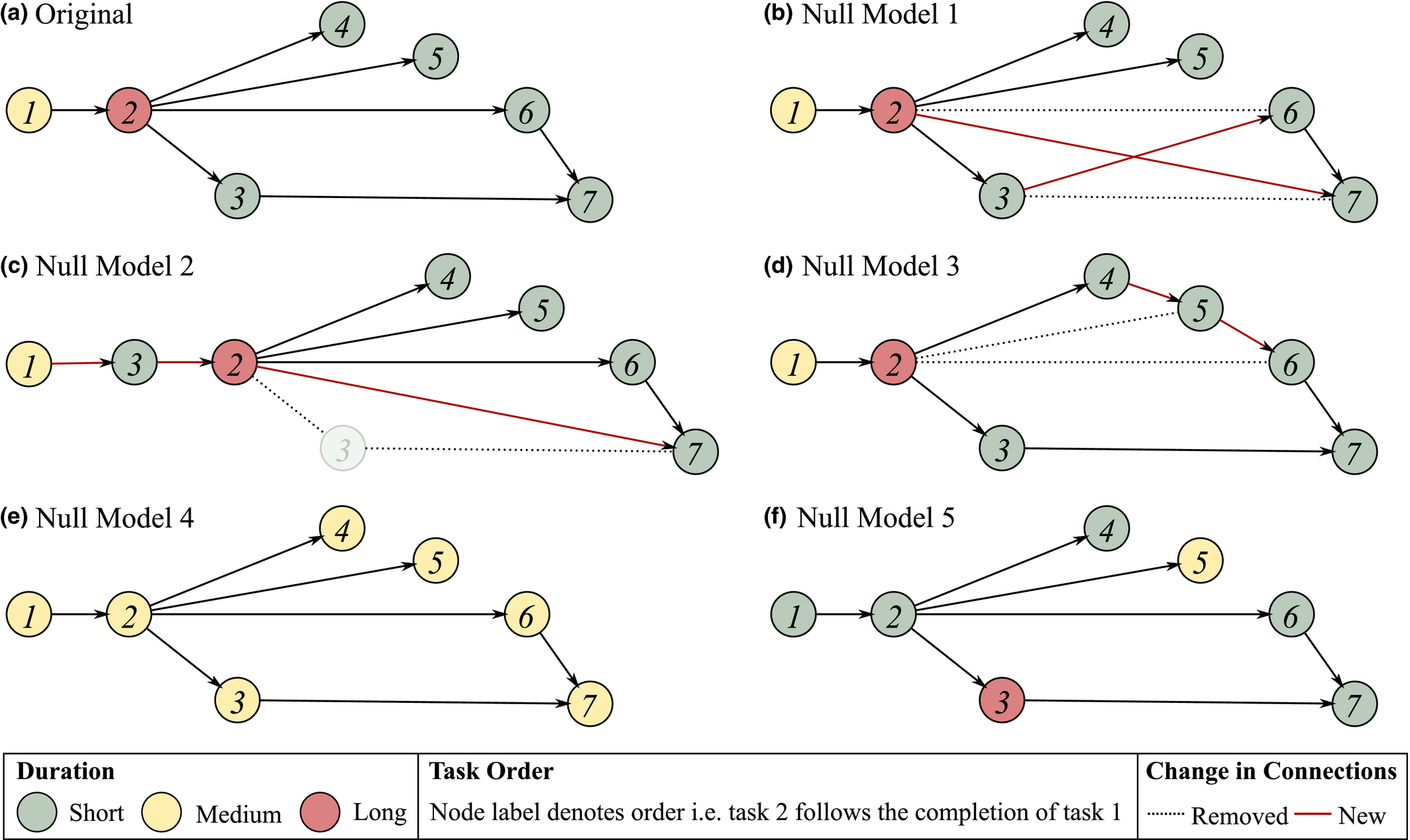
The number of downstream nodes affected by the failure of node i at a given α value is denoted by

C S_{i}^{a}

, with Figure 5a and b visualizing an example of the largest

(C S_{i}^{100} = 467)

and average

({\bar{CS}}_{i}^{100} = 27)

failure cascade, respectively, sustained by the AON network of Project Plan 1. With respect to the capacity of a project to exhibit systemic failures, two points are of particular interest: (i) whether failure cascades of exceedingly large size can occur, and (ii) whether the probability of such cascades to occur is significant. We refer to these aspects as the failure severity and large‐scale failure emergence of a project, respectively.

Figure 5

Subplot (a) and (b) Visualize the Largest and a Typical Failure Cascade across AON Network of Project Plan 1 [Color figure can be viewed at wileyonlinelibrary.com]

Note: Node color corresponds to the state of each node, where gray, red, and blue corresponds to “non‐affected,” “affected,” and the task responsible for triggering the cascade.

To evaluate failure severity and the emergence of large‐scale failures, we obtain the failure cascade distribution from an empirical project, and compare it with an artificial sample, which purposefully scores low in both failure severity and emergence of large‐scale failures. This artificial sample of cascade sizes is one that preserves the same average and variance from the one obtained from the empirical results, yet is unable to exhibit exceedingly large failure cascade sizes, both in terms of increased size and frequency (i.e. failure cascade sizes are normally distributed). This artificial sample essentially corresponds to the case where linearity is assumed, that is, traditional PM methodologies. Hence, if the sample obtained from the empirical set is similar to the artificial set, we can deduce that the particular project is not susceptible to failure cascades, and vice versa.

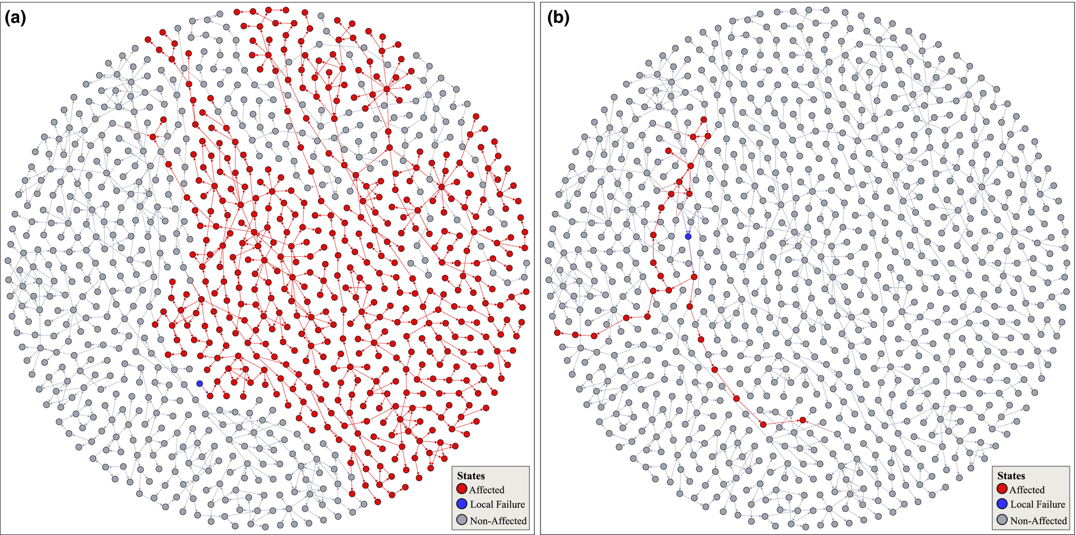
Focusing on failure severity, Figure 6 plots the cumulative probability distribution of failure cascade sizes for Project Plan 1 and 2, under the case of α = 100. The failure cascade size distribution of their artificial counterpart is also included for reference. For the sake of clarity, failure cascade sizes for both the empirical and the artificial set are normalized between 0 and 1, corresponding to the smallest and largest cascade size found within each set of results. Probability plots for the remaining dataset are included in Appendix S1, section 5.

Figure 6

Cumulative Probability Distribution of Cascade Sizes for: (a) Project Plan 1 and (b) Project Plan 2, with Results from the Respective AON Network (Square) and Artificial Sample (Line) [Color figure can be viewed at wileyonlinelibrary.com]

Note: Cascade size is normalized such as 0 and 1 reflects the minimum and maximum cascade size obtained under both empirical and artificial sets respectively. Results are representative of the entire dataset, and correspond to the case of α = 100.

Compared to their artificial counterparts, Project Plan 1 and 2 are capable of sustaining exceedingly large failure (i.e., high X), highlighting their susceptibility to project systemic risk. For example, in the case of Project Plan 1 (Figure 6a), the largest failure cascade size is 167.38% larger from its respective artificial set – a trend which is preserved across the entire dataset (see Table 6). Interestingly, failure severity is preserved regardless of the size of the AON network. Hence, susceptibility to project systemic risk is scale invariant, that is, both small and large projects showcase increasingly high failure severity.

Table 6

Probability of a Failure Cascade of a Given (Normalized) Size in the Empirical Dataset, Compared to its Artificial Counterpart, Where the Latter Essentially Corresponds to a Linear Failure Model

Dataset		Reference quantity
Dataset		$P (X_{i} \geq 0.1)$	$P (X_{i} \geq 0.2)$	$P (X_{i} \geq 0.3)$	$P (X_{i} \geq 0.4)$	$P (X_{i} \geq 0.5)$	$P (X_{i} \geq 0.7)$	$P (X_{i} = 1)$
Project Plan 1	Empirical	1.2 × 10⁻¹	7.2 × 10⁻²	3.5 × 10⁻²	2.6 × 10⁻²	2.0 × 10⁻²	3.4 × 10⁻³	2.3 × 10⁻³
Project Plan 1	Artificial	4.9 × 10⁻¹	1.4 × 10⁻¹	2.1 × 10⁻²	1.6 × 10⁻³	5.3 × 10⁻⁵	0.0	0.0
Project Plan 2	Empirical	2.6 × 10⁻¹	1.2 × 10⁻¹	6.0 × 10⁻²	2.4 × 10⁻²	2.4 × 10⁻²	8.3 × 10⁻³	2.4 × 10⁻³
Project Plan 2	Artificial	5.7 × 10⁻¹	2.2 × 10⁻¹	5.6 × 10⁻²	8.5 × 10⁻³	7.5 × 10⁻⁴	1.2 × 10⁻⁶	0.0
Project Plan 3	Empirical	1.0 × 10⁻¹	5.2 × 10⁻²	2.7 × 10⁻²	1.3 × 10⁻²	1.0 × 10⁻²	6.5 × 10⁻³	1.3 × 10⁻³
Project Plan 3	Artificial	4.2 × 10⁻¹	8.5 × 10⁻²	7.3 × 10⁻³	2.4 × 10⁻²	1.3 × 10⁻⁶	0.0	0.0
Project Plan 4	Empirical	1.1 × 10⁻¹	5.7 × 10⁻²	3.1 × 10⁻²	1.2 × 10⁻²	1.0 × 10⁻²	6.2 × 10⁻³	1.2 × 10⁻³
Project Plan 4	Artificial	4.3 × 10⁻¹	9.0 × 10⁻²	8.1 × 10⁻³	2.8 × 10⁻⁴	6.2 × 10⁻⁶	0.0	0.0
Project Plan 5	Empirical	7.3 × 10⁻²	3.1 × 10⁻²	2.3 × 10⁻²	2.1 × 10⁻²	2.1 × 10⁻²	1.9 × 10⁻²	1.9 × 10⁻³
Project Plan 5	Artificial	4.8 × 10⁻¹	1.4 × 10⁻¹	2.2 × 10⁻²	1.8 × 10⁻³	8.8 × 10⁻⁵	0.0	0.0
Project Plan 6	Empirical	7.3 × 10⁻²	3.1 × 10⁻²	2.3 × 10⁻²	2.1 × 10⁻²	2.1 × 10⁻²	1.9 × 10⁻²	1.9 × 10⁻³
Project Plan 6	Artificial	4.8 × 10⁻¹	1.4 × 10⁻¹	2.1 × 10⁻²	1.8 × 10⁻³	6.9 × 10⁻⁵	0.0	0.0
Project Plan 7	Empirical	2.2 × 10⁻¹	1.5 × 10⁻¹	5.1 × 10⁻²	3.3 × 10⁻²	2.1 × 10⁻²	1.5 × 10⁻²	3.0 × 10⁻³
Project Plan 7	Artificial	5.7 × 10⁻¹	2.2 × 10⁻¹	5.5 × 10⁻²	7.9 × 10⁻³	7.0 × 10⁻⁴	0.0	0.0
Project Plan 8	Empirical	2.3 × 10⁻¹	1.6 × 10⁻¹	7.3 × 10⁻²	4.4 × 10⁻²	2.2 × 10⁻²	1.6 × 10⁻²	3.2 × 10⁻³
Project Plan 8	Artificial	6.3 × 10⁻¹	3.0 × 10⁻¹	1.0 × 10⁻¹	2.4 × 10⁻²	4.0 × 10⁻³	4.1 × 10⁻⁵	0.0
Project Plan 9	Empirical	1.2 × 10⁻¹	4.6 × 10⁻²	2.7 × 10⁻²	1.7 × 10⁻²	1.3 × 10⁻²	5.3 × 10⁻³	1.1 × 10⁻³
Project Plan 9	Artificial	4.3 × 10⁻¹	8.9 × 10⁻²	8.1 × 10⁻³	3.1 × 10⁻⁴	4.3 × 10⁻⁶	0.0	0.0
Project Plan 10	Empirical	1.2 × 10⁻¹	4.6 × 10⁻²	3.1 × 10⁻²	2.3 × 10⁻²	1.7 × 10⁻²	4.8 × 10⁻³	9.6 × 10⁻⁴
Project Plan 10	Artificial	4.3 × 10⁻¹	9.7 × 10⁻²	9.9 × 10⁻³	4.5 × 10⁻⁴	9.6 × 10⁻⁶	0.0	0.0

Focusing on the emergence of large‐scale failures, Table 6 reports the probability of encountering a failure cascade of a given, normalized, size. In the case of large failure cascades – X ≥ 0.4; arbitrary chosen – the difference between the empirical and artificial sample is already severe, with differences in several orders of magnitude being common. For example, the probability of impacting almost half of the maximum number of affected nodes in Project Plan 1 (187 nodes) is three orders of magnitude higher that its artificial counterpart (Figure 6a). In other words, the probability of having a task that can affect 187 downstream tasks is roughly 1000 times higher than what one would normally expect, that is, under the case of linear cause‐and‐effect failures. Table 6 illustrates that this behavior is preserved across the entire dataset, emphasizing the increased susceptibility of projects to large‐scale failure cascades. As with failure severity, the emergence of large‐scale failures is scale invariant, for example, the probability of the AON network from Project Plan 2 to encounter a failure cascade that can affect at least half of the maximum number of downstream tasks is roughly equal with that of Project Plan 10. This is despite the fact that the former (Project Plan 2) is roughly three times larger – and hence, provides the potential for larger cascades to occur – than the latter (Project Plan 10).

Finally, it is worth noting that these results are model‐independent: results do not depend on the particulars of the model (i.e., to the specific aspects incorporated in defining the “spreading power” and “sensitivity” of node i and j respectively). Rather, they correspond to novel, consistent behavior across all projects examined. For the corresponding model robustness analysis see Appendix S1, section 6.

Impact of AON Network Features to Systemic Failures

To assess the influence of particular project features to their susceptibility to failure cascades, let us consider the cumulative probability distribution of failure cascade sizes under different null models, and how they compare against the original AON network of Project Plan 1.

Focusing on the influence of the AON network topology, Figure 7a plots the probability of encountering a failure cascade of a given size in the original project and Null Model 1‐3. At this point, Null Model 2 (no topological correlations; task ordering restriction relaxed) exhibits an almost identical behavior to the original project. Hence, topological correlations, in combination with task ordering, has almost no effect in terms of failure severity and large‐scale failure emergence. However, when examined in isolation, topological correlations reduce both failure severity and large‐scale failure emergence; evident by comparing the original project with Null Model 1 (no topological correlations). In contrast, the existence of the task ordering restriction has a positive effect evident by comparing Null Model 1 (no topological correlations) and Null Model 2 (no topological correlations; task ordering restriction relaxed), where the latter shows an overall improvement in both failure severity and large‐scale failure emergence. Finally, the existence of degree heterogeneity has a worsening effect, where Null Model 1 (no topological correlations) sustains consistently larger failure cascades, occurring at a higher probability, when compared to Null Model 3 (no topological correlation; no degree heterogeneity). In terms of varying the temporal features (Figure 7b), both Null Model 4 and 5 exhibit almost identical behavior with the original project, a result that can be attributed to the fact that under the α = 0 condition, the role of temporal aspects to the cascade dynamics are essentially nullified (see RHS of equation 7).

Figure 7

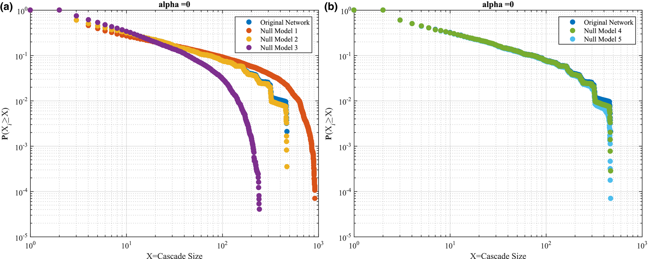
Cumulative Probability Distribution of Failure Cascade Sizes for the Project (Original Network) and Null Models 1–5, Focusing on: (a) Topological, Null Model 1–3, and (b) Temporal Features, Null Model 4–5. This Case is for α = 0 [Color figure can be viewed at wileyonlinelibrary.com]

Results under α = 0 are consistent when α increases to 100, with Null Model 1 showcasing the highest failure severity and large‐scale failure emergence, followed by Null Model 2 and 3 – see Figure 8a. In terms of temporal features, the original project is least susceptible to failure cascades, compared to Null Model 4 and 5, indicating that increased heterogeneity in task duration (Null Model 4) and temporal correlations (Null Model 5) increase susceptibility to failure cascades (Figure 8b). Interestingly, Null Model 4 and 5 preserve the similarity noted when α = 0, muddling our ability to infer the feature with the largest impact. Probing this similarity further, higher values of α shed some light– see Figure 9a and b, where α = 150 and α = 200, respectively. In both cases we note that the temporal correlations dominate over the influence of task duration heterogeneity, evident by the larger difference between the original AON network and Null Model 5, compared to that between the AON network and Null Model 4.

Figure 8

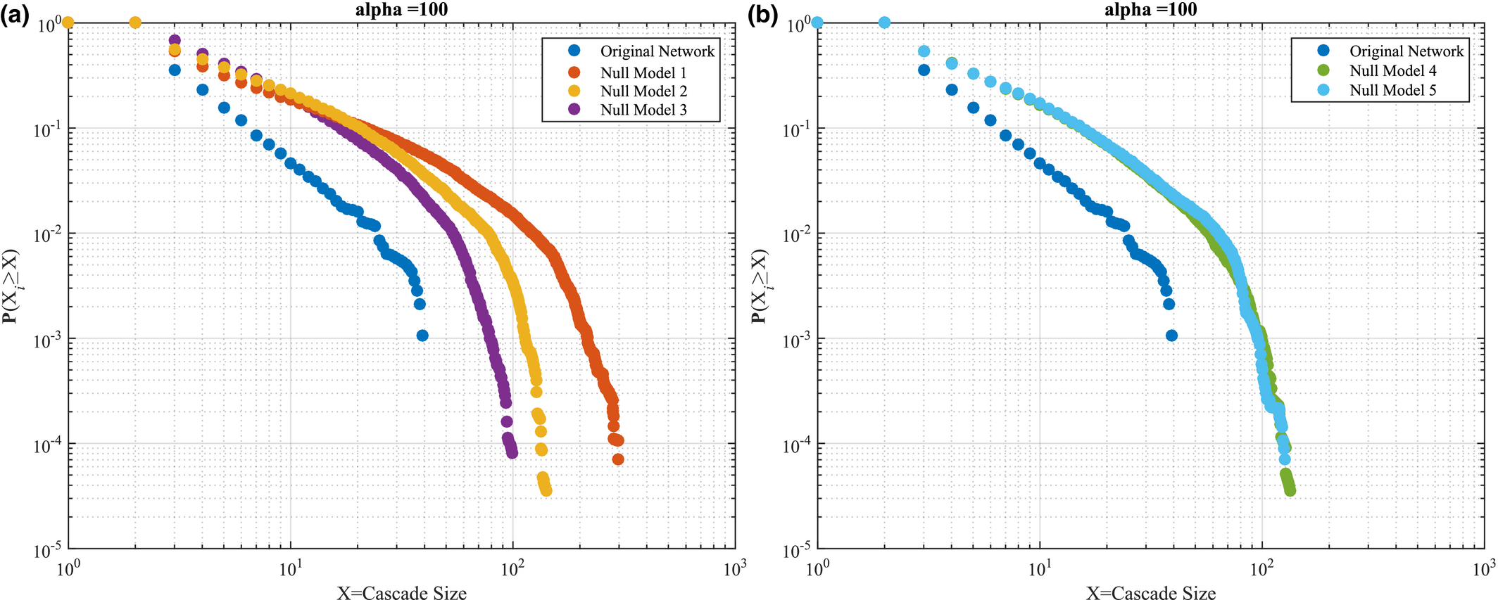
Same as Figure 7, for α = 100 [Color figure can be viewed at wileyonlinelibrary.com]

Figure 9

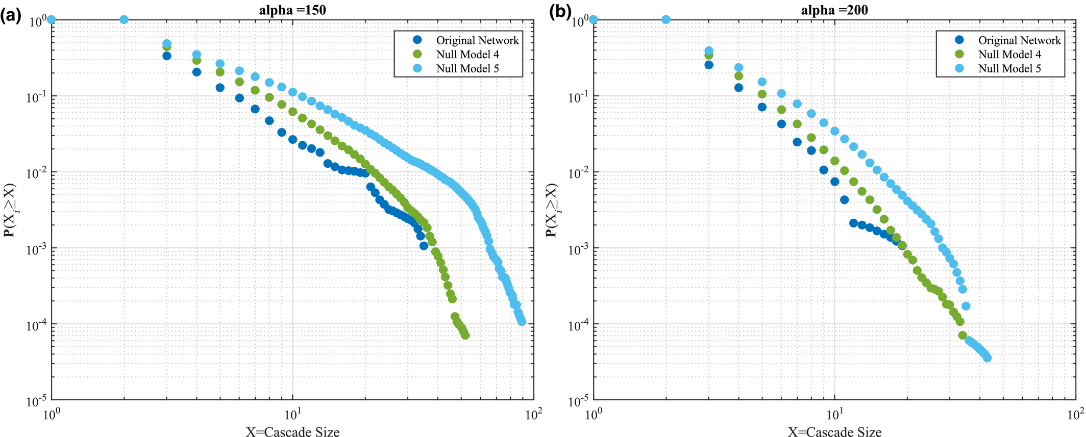
Same as Figure 7, Focusing Solely on Temporal Features for: (a) α = 150 and (b) α = 200 [Color figure can be viewed at wileyonlinelibrary.com]

Effectiveness of Local Mitigation

Allocating extra resources to tasks that benefit the most is a key prerequisite for managing project risk effectively, especially as additional resources are scarce and finite. This effect is modeled by varying parameter α, where a higher value corresponds to an increase in the efficiency by which a task utilizes its resource in order to lower the probability of that task being affected by the failure of some upstream task.

The effectiveness by which an increase in α can contain a particular failure cascade is captured through the relative difference

(R_{ι}^{α})

in cascade size between the mitigated

(C S_{i}^{α})

and unmitigated

(C S_{i}^{0})

case, defined as:

R_{i}^{α} = \frac{C S_{i}^{α}}{C S_{i}^{o}} \times 100, α ϵ [1, 200]

(Buzna et al. 2007). As such, we can distinguish between tasks who benefit from a given level of local mitigation (i.e.,

0 < R_{ι}^{α} < 100

) from those who do not. Note that we ignore tasks with no immediate downstream tasks in order to account for biases that may occur, where the resulting cascade size is always zero – and hence, R _i = 0 – implying that local mitigation has had no effect. Yet this need not be the case, since this instance is merely an artifact of the network topology, that is, nodes with no links cannot trigger a cascade.

The average impact of tasks that benefit from local mitigation

({\bar{CS}}_{l}^{o}, \forall

such that

R_{l}^{α} ϵ (0, 100); normalized over N)

decreases as local mitigation increases – see Figure 10. In detail, and in the spirit of Baños et al. (2013) and Ellinas (2018), we consider the average impact of the tasks that benefit from local mitigation in order to identify whether these tasks are “extraordinary” or “average,” in terms of the cascade size that is triggered from their failure. As such, we note that the average impact of tasks that benefits from low levels of mitigation is initially high – a desirable outcome since these are the tasks which are capable of triggering large‐scale failures. However, as local mitigation increases (i.e., α increases), the average impact of the tasks that benefit from it reduces abruptly, converging to relatively low levels. This behavior is consistent across the entire dataset, and demonstrates the diminishing effectiveness of local mitigation, where tasks that benefit from it can impact only few downstream tasks, on average.

Figure 10

Average Impact of Tasks that Benefit from Local Mitigation of a Given α Level

({\bar{CS}}_{l}^{o}, \forall

such that

R_{l}^{α} ϵ

(0,100)) [Color figure can be viewed at wileyonlinelibrary.com]

Note: Results are Normalized Over the Total Number of Nodes, N, to Allow for Comparison between Projects of Different Size.

Interestingly, the average impact of the tasks that benefit from local mitigation is only slightly higher than the average impact of all tasks – see Appendix S1, section 7. In other words, tasks that benefit from increased mitigation levels are not the extraordinary ones – in terms of ability to trigger large‐scale failures. Rather, these tasks are increasingly similar to the impact of an average task. This is converse to an ideal scenario where local mitigation effectively contains large‐scale failures by benefiting tasks of increased ability to trigger large cascades.

Efficiency of Local Mitigation

The symmetry of the failure cascade size distribution reflects the impact of each individual task failing. Therefore, we can evaluate the impact of local mitigation in smoothening the impact of each individual task by evaluating possible shifts in this symmetry of the failure cascade size distributions, as α increases from 0 to 200. An increase in symmetry suggests that local mitigation is effective in balancing the impact of individual task failure and thus, local mitigation can be considered to be an efficient way of reducing the overall susceptibility of the project to failure cascades, and vice‐versa.

We use the Gini coefficient to evaluate such shifts in symmetry – a measure traditionally used to characterize the equality of wealth distribution in economics. Its value ranges from 0 to 1, which corresponds to a perfectly equal (symmetric) or unequal (asymmetric) distribution, respectively. Applied to the failure cascade size distribution, it can be interpreted as the contribution of each node to the totality of cascade sizes recorded, where a Gini coefficient of 0 indicates that the contribution between nodes is equal. As the value increases, it indicates that the contribution of cascades shifts to an increasingly small subset of nodes. At the limit of where the number of nodes approaches infinity, and only one node capable of triggering a cascade, the Gini coefficient converges to 1. Hence, if an increase in α leads to a reduction in the Gini coefficient, it means that the number of nodes capable of triggering large failure cascades has reduced, resulting to an increasingly symmetric failure cascade size distribution. If that is the case, then it implies that local mitigation is an efficient way of containing failure cascades, with nodes capable of triggering large cascades benefiting the most.

Yet the converse appears to be the case. Specifically, a positive change in the Gini coefficient is noted across almost the entire dataset, with Project Plan 7 and 8 being the sole exception as they experience a slight decrease (see Table 7). In terms of absolute values, Project Plan 5 has the lowest Gini coefficient at α = 0, indicating that the overall capacity to trigger large cascades is equally distributed across all nodes. At this point, each task has a similar capacity to affect the overall project. However, as α increases Project Plan 4 exhibits the largest change in terms of the Gini coefficient. At this point, some tasks have become disproportionality important in terms of their capacity to affect the overall project. In other words, local mitigation has benefitted nodes which trigger small failure cascades more, leading to an increasingly asymmetric distribution of failure cascade sizes. Hence, the impact of local mitigation is distributed in an inefficient way.

Discussion

On Project Susceptibility to Systemic Failures

Projects are traditionally considered to be unique in nature (one‐off) and hence, if large‐scale failure occurs, it can be credited to some exogenous factor(s) that exploited the peculiarities of that project (e.g., see Table 1 in (Zwikael and Globerson 2006)). Results of this work indicate that the converse can also be true, where minor endogenous disturbances – such as a single task failing – can trigger exceedingly large failure cascades, capable of affecting substantial portions of the entire project. The implication of this proposition is that no major exogenous cause or convoluted mechanisms is necessary for a project to fail. In comparison, consider the highly cited work of Pinto and Mantel (1990) which discusses that “unforeseen economic downturns, development of a superior technical alternative, or changes in governmental regulations are among the many reasons project might fail”. Yet this is somewhat expected: extraordinary causes are bound to have an extraordinary effect on a project's performance. Our work provides an alternative scenario, where modest disruption is sufficient for a large‐scale failure to occur, with certain project features serving as key enables (Table 8). This is particular important as the failure of a single task is a more probable failure scenario compared to the extraordinary conditions regularly argued to be the cause of project failure.

Table 7

Contribution of Individual Nodes to the Overall Cascade Sizes; Positive Shift in the Gini Coefficient Indicates a Toward Contribution Inequality

Dataset	Gini coefficient, at α = 0	Gini coefficient, at α = 200	Relative change (%)
Project Plan 1	0.307	0.347	13.05
Project Plan 2	0.305	0.355	16.35
Project Plan 3	0.176	0.345	95.75
Project Plan 4	0.169	0.343	102.86
Project Plan 5	0.102	0.339	231.45
Project Plan 6	0.108	0.336	211.99
Project Plan 7	0.317	0.303	−4.40
Project Plan 8	0.323	0.301	−6.79
Project Plan 9	0.260	0.353	35.60
Project Plan 10	0.308	0.3482	12.94

As a result, decision makers need to account for increased levels of exposure to failure severity and large‐scale failure emergence. With respect to the former (failure severity) the nature of the failure cascade size distributions suggests that the size of the project may be the sole limiting factor for its eventual size, in step with the theoretical work of Clauset et al. (2009). In addition, the difference between average and largest failure cascade size is substantial, with variance ranging from 6 to 14 standard deviations being typical. In terms of the latter (large‐scale failure emergence), large failure cascades are shown to be up to 3 orders of magnitude more likely to occur compared to linear cause‐and‐effect failure scenarios, such as the ones adopted by traditional PM techniques.

In combination, these findings highlight the consistent exposure of projects to systemic risk. Importantly, both failure severity and large‐scale emergence frequency are driven by the rather probable scenario of a single task failing rather than some sort of extraordinary, and hence improbable, scenario. In addition, the nonlinear nature of these failure cascades highlights the limitations of traditional project risk management tools to account for project systemic risk. This is not to say that the techniques themselves are flawed, but to emphasize that project systemic risk is bound to elude identification due to the assumption of linearity that underlies these tools. In response, the application of complex networks in general, and of this work in particular, provide new ways in which project systemic risk can be quantified, and in turn accounted for, using readily available data (e.g., project schedules).

It is worth noting that the majority of tasks have a minimum (or no) impact on the susceptibility of the overall project; thus, one may afford to simply discard their systemic importance. In contrast, a handful of tasks are of great systemic importance, as their individual failure can trigger cascades that resonate deep within the project, by affecting numerous downstream tasks. This insight stresses the importance of identifying and managing impactful tasks on a case by case basis – a “one‐size‐fits‐all” approach will most certainly not suffice. Some tasks are substantially different in terms of their systemic impact and should be treated as such. More generally, one could reasonably postulate that numerous projects have been successfully delivered due to a deep effort in managing these few, impactful tasks – this is in contrast to a uniform but constraint effort across all nodes. Equally, one could also hypothesize that a project may have been successfully delivered simply out of pure luck, as a random failure is more likely to affect a node with limited systemic impact. As a result, causality between best practice and successful project delivery becomes increasingly blurry, challenging our ability to objectively evaluate the utility of various PM techniques.

On Local Mitigation and its Effect

Local mitigation is typically deployed under the assumption that benefits will aggregate from the task level to the project level, that is, improving individual task performance improves the overall project performance. In the context of failure cascades, this assumption suggests that local mitigation can contain the emergence of large‐scale failures. With that in mind, high effectiveness corresponds to the ability of local mitigation to contain cascades that stem from the failure of tasks that have the capacity to trigger large‐scale failures. Yet the converse appears to be the case, where increased mitigation benefits tasks that, on average, have limited overall impact. Increasing the level of mitigation has little effect over this consistent behavior, with the average impact of the benefiting tasks being marginally higher than that of an average task.

Shifting focus from mitigation effectiveness to mitigation efficiency, results in Table 7 suggest that local mitigation benefits tasks that are of little importance, in terms of their ability to trigger large failure cascades. In other words, the benefits that result from the application of local mitigation is distributed in an inefficient way. This is in contrast to what a decision maker would strive for, as tasks capable of triggering large‐scale failures show little improvement.

Table 8

Summary of the Impact of Each Project Features on Susceptibility to Failure Cascades. Results are Consistent across the Entire Spectrum of α

Presence of specific feature		Impact on failure cascade susceptibility
Topological	Topological correlations	Reduces susceptibility
	Task order	Increases susceptibility
	Degree heterogeneity	Increases susceptibility
Temporal	Duration heterogeneity	Increases susceptibility
Temporal	Temporal correlations	Increases susceptibility

Managerial Insight

Relating network features that control susceptibility to failure cascades to actionable insight can be of great practical value, as they suggest a way of reducing both failure severity and the emergence of large‐scale failures. This is in contrast to the case of having to deal with extraordinary conditions, which tend to be generic in nature, and therefore limiting in terms of actionable mitigation (Zwikael and Globerson 2006). With that in mind, and in reference to Table 8, project managers and relevant stakeholders should amend project schedules, wherever possible, in order to:

Reduce variance in task duration: a project composed of many quick tasks, and few surprisingly long tasks will be exceedingly susceptible to large‐scale failures, compared to one in which tasks are of similar duration;

Recommendation: Strive for standardized delivery processes, which can normalize time for delivery across the project;

Reduce variance throughout task interdependencies: a project composed of many tasks with few functional dependencies, and some with surprisingly high connections will be exceedingly susceptible to large‐scale failures;

Recommendation: Reduce functional interdependences between tasks by: (a) optioneering the design of the final artifact, and (b) outsourcing tasks with high functional dependencies (assuming different contractors will be involved);

Reduce temporal “burstiness” in scheduled activity: a project composed of concentrated planned activity with intermediate long pauses, is increasingly susceptible to failure cascades, compared to one in which tasks completion progresses at a steady rate;

Recommendation: Focus on enabling logistical aspects (e.g., cash flow) and contracting activity (e.g., their mixing patterns (Ellinas et al. 2016a) that can enable an increasingly steady rate of task completion across the project.

In addition to these specific recommendations, more general insight can be produced. For example, project schedules that satisfy a large number of conditions responsible for increased susceptibility to failure cascades (Table 8) should be treated as more “complex” and therefore, suitably amend their (a) contingency budget, (b) risk management and governance framework and (c) stakeholder involvement, to reflect this.

Limitations and Further Work

Several extensions deserve further exploration in order to better understand the link between AON networks and project performance. Of particular interest is working towards establishing the universality of the insights presented herein, especially with respect to the noted failure severity and the emergence of large‐scale failures. For example, the lack of a generative model that can reconstruct realistic AON networks means that empirical data remain the sole source of AON networks. This limitation implies that the universality of our findings may be restricted to this particular dataset. However, the consistency by which our findings apply across seemingly distinct projects support the wider nature of the insights presented herein, and justify further exploration due to the important practical implications.

Another fruitful direction would be to establish the conditions in which local action (task mitigation) promotes desirable behaviors at the macrolevel (containing large‐scale cascades) in an effective and efficient way. Our findings suggest that deploying local mitigation in a uniform way is neither of the two, and is in step with recent findings across a range of domains, from ecology to logistics and supply chains (Gershenson and Helbing 2015). Yet work around establishing the origin of these phenomena – including the results herein – can only be viewed as preliminary, since no causal links has yet been established in terms of the specific aspects that drive these effects. Therefore, there is a need to better understand, and eventually map, the conditions that drive these effects, and subsequently develop tools that overcome them. This is particularly important in the context of PM specifically, and management science in general, where the action of decision makers is often limited to the local level.

On the practical front, exploiting insight around project features that control their susceptibility to failure cascades can be exceedingly challenging, largely due to the intrinsic limitations in amending certain project features. For example, consider the case of task degree heterogeneity – a decision maker will have limited capabilities in terms of amending it due to limitations in controlling the functional dependencies between tasks. Yet, illustrating that these features are catalytic in terms of projects systemic risk can be used to reduce project uncertainty across a wide range of aspects, from project bidding and setting up appropriate regulatory frameworks to sizing‐up contingency budgets.

Conclusion

Shielding projects from large‐scale failures is a persistent challenge for both practitioners and academics. The convoluted nature of such failures challenges our ability to identify their root cause. As a result, decision makers typically invoke extraordinary – and often, project dependent – conditions in order to guide project risk management. This work adopts a distinctly different view, where large‐scale failures arise from modest disruptions, in the form of a single task failing – an increasingly probable scenario compared to the aforementioned case of extraordinary conditions.

In sum, our work makes three contributions. First, we develop a computational model capable of replicating large‐scale, project failures, in the form of failure cascades. This model makes it possible to evaluate, in a systematic manner, the susceptibility of real‐world projects to these failure cascades, using readily available data (AON networks). Focusing on engineering projects, we illustrate that they are increasingly exposed to large‐scale failure cascades (failure severity), which occur at a surprisingly high rate (large‐scale failure emergence). Second, as summarized in Table 8, we associate failure severity and large‐scale failure emergence to particular project characteristics. These associations can help translate this theoretical contribution to actionable insight by suggesting ways of configuring projects in order to reduce susceptibility to failure cascades. Furthermore, these associations become particular relevant when considered in conjunction with our third contribution, in which we show that local mitigation is both ineffective and inefficient in containing the severity and emergence of these large‐scale failures. Considering the fact that managers are typically limited to such local action, it is important to realize that benefits that may result from such local action (e.g., increased resource efficiency) do not necessarily aggregate to the project level (e.g., improved robustness to large‐scale failures).

More generally, our work serves as an example of how interdisciplinary approaches can improve our understanding around the complex nature of modern projects, supplementing traditional and well‐established risk management approaches. It further calls for an embrace of nonlinearity and complexity as actualities of modern projects and invites an exploration of their implications – a much neglected yet increasingly relevant facet of PM.

Footnotes

Acknowledgments

Data contribution by Lois Builders Ltd is gratefully acknowledged. The author is particularly thankful to the department editor, senior editor and the two anonymous reviewers for their insightful comments. This work was supported by EPSRC under grant EP/N509619/1. The funders had no role in the design, data collection and analysis of this work.

ORCID

Christos Ellinas

References

Albert

Jeong

Barabási

A.‐L.

. 2000. Error and attack tolerance of complex networks. Nature. 406(6794): 378–382.

Bak

Paczuski

. 1995. Complexity, contingency, and criticality. Proc. Natl. Acad. Sci. 92(15): 6689–6696.

Bak

Tang

Wiesenfeld

. 1987. Self‐organized criticality: An explanation of the 1/f noise. Phys. Rev. Lett. 59(4): 381–384.

Baños

R. A.

Borge‐Holthoefer

Moreno

. 2013. The role of hidden influentials in the diffusion of online information cascades. EPJ Data Sci. 2(1): 6.

Battiston

Puliga

Kaushik

Tasca

Caldarelli

. 2012. “Debtrank: Too central to fail? Financial networks, the fed and systemic risk.” Scientific reports 2.

Browning

T. R.

Ramasesh

R. V.

. 2007. A survey of activity network‐based process models for managing product development projects. Prod. Oper. Manag. 16(2): 217–240.

Buldyrev

S. V.

Parshani

Paul

Stanley

H. E.

Havlin

. 2010. Catastrophic cascade of failures in interdependent networks. Nature 464(7291): 1025–1028.

Buzna

Peters

Ammoser

Kühnert

Helbing

. 2007. Efficient response to cascading disaster spreading. Phys. Rev. E 75(5): 056107.

Clauset

Shalizi

C. R.

Newman

M. E.

. 2009. Power‐law distributions in empirical data. SIAM Rev. 51(4): 661–703.

10.

Cullen

. 1990. The public inquiry into the Piper Alpha disaster (Report to the Parliament by the Secretary of State for Energy by Command of Her Majesty Vols. 1 and 2), HMSO, London.

11.

Ellinas

2018. Modelling indirect interactions during failure spreading in a project activity network. Sci. Rep. 8(1): 4373.

12.

Ellinas

Allan

Johansson

. 2016a. Project systemic risk: Application examples of a network model. Int. J. Prod. Econ. 182: 50–62.

13.

Ellinas

Allan

Johansson

. 2016b. Toward project complexity evaluation: A structural perspective. IEEE Syst. J. 12(1): 228–239.

14.

Ellinas

Allan

Johansson

. 2017. Dynamics of organizational culture: Individual beliefs vs. social conformity. PLoS ONE 12(6): e0180193.

15.

Geraldi

Maylor

Williams

. 2011. Now, let's make it really complex (complicated) a systematic review of the complexities of projects. Int. J. Oper. Prod. Manag. 31(9): 966–990.

16.

Gershenson

Helbing

. 2015. When slower is faster. Complexity 21(2): 9–15.

17.

Granovetter

. 1978. Threshold models of collective behavior. Am. J. Sociol. 83: 1420–1443.

18.

Gunasekaran

Ngai

E. W.

. 2012. The future of operations management: An outlook and analysis. Int. J. Prod. Econ. 135(2): 687–701.

19.

Harrison

J. R.

Lin

Carroll

G. R.

Carley

K. M.

. 2007. Simulation modeling in organizational and management research. Acad. Manag. Rev. 32(4): 1229–1245.

20.

Herroelen

Leus

. 2001. On the merits and pitfalls of critical chain scheduling. J. Oper. Manag. 19(5): 559–577.

21.

Jalili

Ford

D. N.

. 2016. Quantifying the impacts of rework, schedule pressure, and ripple effect loops on project schedule performance. Syst. Dynam. Rev. 32(1): 82–96.

22.

Jarratt

Eckert

C. M.

Caldwell

N. H.

Clarkson

P. J.

. 2011. Engineering change: An overview and perspective on the literature. Res. Eng. Design 22(2): 103–124.

23.

Kappelman

L. A.

McKeeman

Zhang

. 2006. Early warning signs of IT project failure: The dominant dozen. Inf. Syst. Manag. 23(4): 31–36.

24.

Kermack

W. O.

McKendrick

A. G.

. 1932. Contributions to the mathematical theory of epidemics. II—The problem of endemicity. Proc. R. Soc. Lond. A 138. https://doi.org/10.1098/rspa.1932.0171

25.

Kim

Chen

Y.‐S.

Linderman

. 2015. Supply network disruption and resilience: A network structural perspective. J. Oper. Manag. 33: 43–59.

26.

Krishnan

Eppinger

S. D.

Whitney

D. E.

. 1997. A model‐based framework to overlap product development activities. Management Sci. 43(4): 437–451.

27.

Loch

C. H.

Terwiesch

. 1998. Communication and uncertainty in concurrent engineering. Management Sci. 44(8): 1032–1048.

28.

Maytorena

Winch

G. M.

Freeman

Kiely

. 2007. The influence of experience and information search styles on project risk identification performance. Eng. Manag. IEEE Trans. 54(2): 315–326.

29.

McAteer

R. J.

Aschwanden

M. J.

Dimitropoulou

Georgoulis

M. K.

Pruessner

Morales

Ireland

Abramenko

. 2015. 25 years of self‐organized criticality: Numerical detection methods. Space Sci. Rev. 198(1–4): 217–266.

30.

Mihm

Loch

Huchzermeier

. 2003. Problem–solving oscillations in complex engineering projects. Management Sci. 49(6): 733–750.

31.

NASA . 2013. The Case for Safety: The North Sea Piper Alpha Disaster. NASA Safety Center, System Failure Case Study, 7.

32.

Parvan

Rahmandad

Haghani

. 2015. Inter‐phase feedbacks in construction projects. J. Oper. Manag. 39: 48–62.

33.

Pastor‐Satorras

Vespignani

. 2001. Epidemic spreading in scale‐free networks. Phys. Rev. Lett. 86(14): 3200.

34.

Pastor‐Satorras

Castellano

VanMieghem

Vespignani

. 2015. Epidemic processes in complex networks. Rev. Mod. Phys. 87(3): 925.

35.

Pinto

J. K.

Mantel

S. J.

Jr . 1990. The causes of project failure. Eng. Manag. IEEE Trans. 37(4): 269–276.

36.

PMI . 2008. A Guide to the Project Management Body of Knowledge: PMBOK^® Guide, Project Management Institute.

37.

Porter

M. A.

Gleeson

J. P.

. 2016. Dynamical Systems on Networks. Switzerland, Springer, Cham.

38.

Rahmandad

Sterman

. 2008. Heterogeneity and network structure in the dynamics of diffusion: Comparing agent‐based and differential equation models. Management Sci. 54(5): 998–1014.

39.

Schilling

M. A.

Phelps

C. C.

. 2007. Interfirm collaboration networks: The impact of large‐scale network structure on firm innovation. Management Sci. 53(7): 1113–1126.

40.

Schmidt

Lyytinen

Keil

Cule

. 2001. Identifying software project risks: An international Delphi study. J. Manag. Inf. Syst. 17(4): 5–36.

41.

Schweitzer

Fagiolo

Sornette

Vega‐Redondo

Vespignani

White

D. R.

. 2009. Economic networks: The new challenges. Science 325(5939): 422.

42.

Shenhar

A. J.

2001. One size does not fit all projects: Exploring classical contingency domains. Management Sci. 47(3): 394–414.

43.

Sosa

M. E.

2014. Realizing the need for rework: From task interdependence to social networks. Prod. Oper. Manag. 23(8): 1312–1331.

44.

Tavares

L. V.

Wegłarz

. 1990. Project management and scheduling: A permanent challenge for OR. Eur. J. Oper. Res. 49(1): 1–2.

45.

Terwiesch

Loch

C. H.

. 1999. Managing the process of engineering change orders: The case of the climate control system in automobile development. J. Prod. Innov. Manag. 16(2): 160–172.

46.

Turner

Müller

. 2005. The project manager's leadership style as a success factor on projects: A literature review. Project Manag. J. 36(2): 49–61.

47.

Tversky

Kahneman

. 1974. Judgment under uncertainty: Heuristics and biases. Science 185(4157): 1124–1131.

48.

Valls

Lino

. 2001. Criticality analysis in activity‐on‐node networks with minimal time lags. Ann. Oper. Res. 102(1–4): 17–37.

49.

Vanhoucke

2010. Using activity sensitivity and network topology information to monitor project time performance. Omega 38(5): 359–370.

50.

Vanhoucke

. 2013. An overview of recent research results and future research avenues using simulation studies in project management. ISRN Computational Mathematics 2013.

51.

Vespignani

2012. Modelling dynamical processes in complex socio‐technical systems. Nat. Phys. 8(1): 32–39.

52.

Watts

D. J.

2002. A simple model of global cascades on random networks. Proc. Natl. Acad. Sci. 99(9): 5766–5771.

53.

Watts

D. J.

2014. Common sense and sociological explanations. Am. J. Sociol. 120(2): 313–351.

54.

Williams

T. M.

1999. The need for new paradigms for complex projects. Int. J. Project Manage. 17(5): 269–273.

55.

Williams

T. M

. 2002. Modelling Complex Projects, John Wiley & Sons, New Jersey.

56.

Zwikael

Ahn

. 2011. The effectiveness of risk management: An analysis of project risk planning across industries and countries. Risk Anal. 31(1): 25–37.

57.

Zwikael

Globerson

. 2006. From critical success factors to critical success processes. Int. J. Prod. Res. 44(17): 3433–3449.

58.

Zwikael

Sadeh

. 2007. Planning effort as an effective risk management tool. J. Oper. Manag. 25(4): 755–767.

The Domino Effect: An Empirical Exposition of Systemic Risk Across Project Networks

Abstract

Keywords

Introduction

The Conditions of Project Systemic Risk

Experimental Design

Data

Notes

Overview of the Cascade Model

Definition of Cascade Model Components

Quality of Completion

Spreading Power of Node i

Sensitivity of Node j

Cascade Model Dynamics

Features that Control Project Susceptibility

Results

Evaluating Project Susceptibility to Systemic Failures

Impact of AON Network Features to Systemic Failures

Effectiveness of Local Mitigation

Efficiency of Local Mitigation

Discussion

On Project Susceptibility to Systemic Failures

On Local Mitigation and its Effect

Managerial Insight

Limitations and Further Work

Conclusion

Footnotes

Acknowledgments

ORCID

References