Sage Journals: Discover world-class research

Abstract

Class imbalance can present a major issue in time-to-event analyses for instances where the number of individuals diagnosed with a disease are far outnumbered by those who remain undiagnosed within a specified time frame. An example of this is the incidence rate of myocardial infarction (MI) among patients with stable coronary heart disease, where MI events are typically sparse over the course of a study. This imbalance may result in inaccurate risk predictions for individuals who are more likely to be having an MI event. In this study, we combine sampling with the Cox proportional hazards model in a cross-validation framework to balance predictive performance. This approach leverages advantages provided by classification tools and the statistical power of survival models in examining time-to-event data. To demonstrate the effectiveness of this modeling approach, we use high-dimensional proteomic data (obtained using the SOMAScan^® assay) to identify patients likely to experience an MI event within 4 years of a blood draw. In our data set, 8.1% of patients experienced an MI within 4 years, making this a severely class-imbalanced data set. Cox proportional hazards elastic net regression models were developed using sampling techniques, allowing us to identify and select features that more accurately identify individuals at higher risk of MI. The resulting Cox elastic net regression models created on the sampled data (both upsampled and downsampled) were superior to three other competing models: elastic net logistic regression and support vector machine models developed on downsampled data, and a Cox proportional hazards elastic net developed on the full data. These results, and additional simulation results, demonstrate the effectiveness of combining sampling with survival analysis techniques for improved predictive performance in a biomedical application.

Introduction

Coronary heart disease (CHD) remains a major public health challenge, and is responsible for approximately one-third of deaths in middle-aged and older adults in the United States.¹ CHD is a broad disease, encompassing dietary, lifestyle, and genetic risks, as well as several chronic or acute outcomes, including heart failure, stroke, or myocardial infarction (MI). The phenotypic and genotypic complexity of the disease makes it an ideal target for biomarker discovery, increasingly augmented by high-throughput omics technology.² In previous study, the SOMAScan^® proteomic assay was used to identify protein biomarkers associated with risk of cardiovascular events in patients with stable CHD.^3,4 The resulting model provides improved ability over existing clinical-risk tools and has broad applicability and generalizability among a composite end-point of cardiovascular events.

Diagnosis of a disease with multiple possible outcomes combined with high-dimensional data such as proteomics is both a challenging problem and rich opportunity in translational medicine. In this study, we focus on a targeted model for predicting MI among patients with stable CHD. We used proteomic data to identify patients likely to experience MI within 4 years of a blood draw among patients with stable CHD. In addition to proteomic signals, the data contain information on whether or not specific cardiovascular events occurred over the course of observation, and the length of time to either, (1) the event or, (2) exiting the study due to other factors. These time-to-event data make the problem well suited to survival analysis techniques.

When the primary goal is the correct identification of individuals who will have an MI event within a given time frame (i.e., 4 years), the analysis can be reframed as a classification problem, where individuals are the “positive” class if the event occurred before 4 years, and individuals are labeled as the “negative” class if the individual remained in the study beyond the 4-year time frame with no MI. Survival analysis methods will improve predictive accuracy of the model (compared with classification) because survival models “use all the information” by incorporating the time to MI in development of the classifier and, more importantly, by accounting for subjects with unknown event times (known as “censoring”).^5–9 This reframing also allows us to use standard classification metrics, such as the area under the curve (AUC) and the confusion matrix to assess model performance.¹⁰ This method of assessing survival models is not a traditional approach, but event-specific classification provides a number of benefits in a clinical setting. Labeling a patient as “positive” or “negative” is more easily understood across a wide audience (compared with, e.g., a hazard-ratio or probability). This improved comprehension of a prognostic test allows clinicians to provide precise targeted medical management. However, as with standard classification modeling, this approach to survival analysis can suffer from an imbalance in patients who do and do not experience events.

The effects of class imbalance in classification modeling have been recognized across many different domains.^11–17 Predictive classifiers generally perform poorly on imbalanced data, as the model is trained to be accurate “as often as possible.”^18,19 This effect occurs because the larger majority class drives the features selected for the model, as the minority class can be misclassified frequently without much penalty on the AUC. However, sensitivity and specificity will become imbalanced, such that one is maximized over the other depending on which group has a greater number of observations. In modeling health outcomes, it is common to have low disease prevalence within a cohort, forming the minority class. Specificity will be maximized at the expense of sensitivity, which is problematic when the goal is to identify as many individuals as possible who are at risk for an event. Although there are a number of approaches to resolving this issue, a common approach is to sample the data by either downsampling the majority class or upsampling the minority class.¹⁰ The aim of sampling is to “bias” the classifier so that it pays equal attention to individuals with and without events to balance sensitivity and specificity. Sampling in classification modeling has long been established (see Kubat and Matwin,²⁰ Pazzani et al.,²¹ Japkowicz²² for some of the initial study on this topic) and is frequently used today (see Kuhn and Johnson¹⁰ and Chawla²³). Sampling techniques have been applied to various machine-learning methodologies, but to our knowledge, class imbalance is largely an unexplored topic in machine learning using survival modeling techniques.^{6,15–17,24–27}

We explore sampling techniques combined with a Cox proportional hazards elastic net regression model, and assess prediction of an MI event within 4 years of initial blood draw.^28–31 Our purposes are twofold: (1) selection and identification of features that predict both the minority and majority classes, and (2) derivation of estimated effect sizes such that the risk for the minority class is well predicted. This study contributes to a growing field of scientific research⁶ that combines existing machine learning models with classic survival analysis techniques for more powerful analyses of complex time-to-event data. This article is organized as follows: Materials and Methods section describes the data and modeling approach, Results section reports simulated and clinical data analysis, Discussion section discusses the results, and Conclusion section summarizes the study and suggests future research.

Materials and Methods

Data set

The subjects used in our analyses are a subcohort from the HUNT3 study, a prospective cohort study from Norway that included blood samples drawn from participants and follow-up health information.³² The CHD subcohort is described previously with inclusion criteria as evidence of existing but stable CHD through a history of an MI >6 months prior; or stenosis, inducible ischemia, or previous coronary revascularization.³ Plasma samples were assayed using the SOMAscan Assay (SomaLogic, Inc., Boulder, CO), which uses Slow Offrate Modified Aptamer (SOMAmer^®) reagents to measure relative protein abundance, as hybridized on a custom DNA microarray and reported in continuous relative fluorescence units. The current version of the assay measures ∼5000 unique protein analytes and is a well-established platform for protein biomarker discovery.³³

In this data set, 8.1% of patients experienced an MI within 4 years (Table 1). The Kaplan–Meier survival curve, a nonparametric method for examining how the probability of being event-free changes over time, is depicted in Figure 1 for MI events.³⁴ There is a gradual decrease in the probability of being event free for MI in the CHD subcohort of the HUNT3 data set. Table 1 shows incidence of MI and demographic information for the subcohort.

FIG. 1.

Kaplan–Meier survival curve for MI in the HUNT3 CHD subcohort. CHD, coronary heart disease; MI, myocardial infarction.

Table 1.

Demographic Characteristics for HUNT3 Stable Coronary Heart Disease Subcohort

Characteristic	MI within 4 years	Non-MI within 4 years	No event (MI or other) >4 years	Total	Cases vs. controls
Number of subjects (% total)	61 (8.1)	189 (25.0)	506 (66.9)	756 (100)
Gender
Female (% of group)	20 (32.8)	57 (30.2)	128 (25.3)	205 (27.1)	χ²=0.79 (p<0.37)
Male (% of group)	41 (67.2)	132 (69.8)	378 (74.7)	551 (72.9)
Mean age, years (±SD)	72.6±11.1	72.8±10.3	67.7±10.2	69.4±10.5	t=2.39 (p<0.02)
Time-to-event, years (IQR)	1.93 (1.97)	2.57 (2.73)	4.69 (0.75)	4.37 (1.06)

IQR, interquartile range; MI, myocardial infarction; SD, standard deviation.

In addition to the HUNT3 data set, we generated 100 data sets with 10,000 simulated samples each, with event times and censoring rates similar to the HUNT3 data. Further details on the algorithm used to generate these data sets are given in Supplementary Data of the Algorithm for Simulation section. The results of our models on these simulated data sets are reported in Simulation Results section.

Cox elastic net models

Survival data are characterized through a survival function, S(.), which is the probability of being event free and is calculated at time point t as $S (t) = P r (T > t) = \int_{t}^{\infty} f (u) d u,$

where f(u) is the probability density function of time to event. In addition to the survival function, we are typically interested in the identification and characterization of features that significantly increase or decrease time to event.

A key feature of time-dependent data is that the event will not be observed for some individuals if it occurs outside the study period. These individuals are censored, which can occur for multiple reasons (e.g., death from non-MI causes, individuals withdrawing from the study, and MI occurring after the study window ending). Although there are multiple types of censoring, this study comprises right-censored individuals, meaning that for patients who do not have an MI event, it is assumed to have occurred after the last observed time point. Because survival models can account for different types of censoring, they are different from classification models and should be used when analyzing time-to-event data.

Although there are numerous survival analysis techniques, one of the most common is the Cox proportional hazards model, which is the method of focus for this article.²⁸ (See Supplementary Data of the Cox Proportional Hazards Model section for an in-depth description of Cox models.) However, as with other classical statistical modeling approaches, the Cox model can also suffer when the number of features is greater than the sample size (as is the case with these data). Thus, we use the Cox elastic net proportional hazards model, implemented through the glmnet package available in CRAN-R.^{29–31,35,36} In essence, the Cox elastic net model combines the Cox proportional hazards approach with the elastic net penalty, allowing us to use a regularized regression tool in a survival model context (Detailed in Supplementary Data of the Cox Proportional Hazards Model and Elastic Net sections).^28,29

Sampling methods

The primary focus of the analyses was to mitigate class imbalance for survival data. The use of Cox proportional hazard elastic net models in conjunction with sampling techniques allowed for identification of features that best predict whether an individual is at “high risk” of having an MI event within 4 years. In this study, the “high-risk” classifier was calculated using a hazard ratio threshold identified through cross-validation. Using this technique, we can select features that are useful in identifying high-risk individuals in a way that would be more difficult if we used all the data. In addition, this technique estimated the feature effects in a way that allows features that accurately predict high-risk individuals to have different “weights” (i.e., β estimates) than they would if derived using the full cohort.

Sampling routines were implemented within cross-validation, meaning that the sampling occurred within each cross-validation fold (five repeats of fivefold cross-validation). This approach is particularly important for downsampling to allow more of the data to be utilized across folds. For upsampling, sampling with replacement was used. The elastic net model tuning parameters of alpha and lambda were selected through cross-validation by optimizing misclassification rates across folds and repeats. See Supplementary Data of the Cross-Validation section for a detailed description of the cross-validation procedure.

Analyses were performed using R version 3.4.4 in RStudio server version 1.1.453.^36,37

Data subsetting

Both the HUNT3 data set and simulated data sets were split into a training set (80%) and a test set (20%) stratified by MI event to maintain event distribution across training and test sets. Other splits are possible, but for demonstration purposes a common 80/20 split was examined.³⁸ The training set was used for model building and final models were evaluated on the test set. Thresholds for prediction on the test set for Cox elastic net models were calculated as the average of the thresholds generated per fold during cross-validation. Univariate filtering (t-tests) was performed before modeling using the training set to reduce the feature space and remove features that largely reflect noise.¹⁰ The top 100 analytes ranked by false discovery rate³⁹ values were included for model development. Despite older age individuals being at higher risk for MI, the top 100 associated proteomic features are more significantly associated with outcome than age alone, and thus the resulting model was based only on proteomic features.

Workflow

Across all models presented in the results, we used cross-validation on the training set to select the optimal models within each model type. Feature selection, estimated effects, and classification thresholds were allowed to differ across models. After cross-validation, the best model in each category was evaluated on the test set. The survival models were optimized using the AUC metric at the 4-year time point. This means that a standard survival model was built, but a binary 4-year-mark classifier (yes/no MI before 4 years) was used to calculate AUC and optimize the model. The 4-year outcome was also used to optimize the AUC of the classification models. CIndex⁴⁰ was calculated for survival models to allow model comparison using a standard survival concordance metric.^41–43 For the remainder of the article, for simplicity of notation, we refer to the Cox elastic net models as “Coxnet,” elastic net logistic regression models as “LRnet” and support vector machines as “SVMs.” For models that are downsampled and upsampled, we prepend “DS” and “US,” respectively.

Results

In this section, we present two sets of results. The first set of results are for a simulation, which was performed to demonstrate the generalizability of the method and differences in the survival model results calculated on full data and on sampled data. The second set of results is for the HUNT3 data set analysis.

Simulation results

US and DS-coxnets outperform standard coxnet models across all metrics with the simulated data, thus demonstrating the efficacy of sampling with survival analysis. Supplementary Figures S1 and S2, and Supplementary Tables S1–S4 show the results of the simulations.

Analysis of HUNT3 research study data

We now discuss the results of our analyses of the HUNT data using sampling techniques. In this section, we examine both DS- and US-Coxnet models, a Coxnet model developed on the full data, as well as a DS-LRnet and DS-SVM classification model^44,45 all implemented through the caret package in R. All comparison models use the same cross-validation approach described in the Supplementary Data and in the Workflow section above. To be clear, time-to-event data are often best assessed and compared using survival methods that take into account censoring and other important components of time-to-event analyses.^5–9 However, for the sake of comparison in this article, we also examine two popular classification methods.

Model results and comparison

Cross-validation results show that the US-Coxnet and DS-Coxnet models outperform DS-LRnet and DS-SVM models (Table 2). This result is expected, as survival analysis methods use the time-to-event information as part of feature selection and model development. A more compelling result is that both the DS-Coxnet and US-Coxnet models outperform the DS-LRnet, DS-SVM and standard Coxnet models across all classification metrics (AUC, sensitivity, specificity; Table 2). The DS-Coxnet and US-Coxnet models have a higher C-Index than the standard Coxnet model, indicating that sampled models better predict the ordering of MI event times. The predictive abilities of the top models were evaluated on the test set, including an examination of sensitivity and specificity based on correctly predicting an individual at “high risk” of having an MI within 4 years. Performance metrics for all models on the test set are shown in Table 3. Taken together, the combination of resampling and elastic nets in time-to-event data improves performance in imbalanced data, compared with standard techniques of resampling in classification models, and/or elastic net Cox models. Notably, DS-Coxnet shows a significant increase in sensitivity (0.46 vs. 0.39) compared with the other models (Table 3).

Table 2.

Cross-Validated Training Set Results, Using Five Repeats of Fivefold Cross-Validation

Model	Tuning parameters	AUC	Sensitivity	Specificity	C-Index
Downsampled Coxnet	α=0.75, λ=0.1	0.78	0.74	0.79	0.74
Upsampled Coxnet	α=0.75, λ=0.1	0.82	0.88	0.75	0.80
Coxnet	α=0.75, λ=0.05	0.61	0.67	0.66	0.58
Downsampled logistic regression	α=0.75, λ=0.05	0.75	0.65	0.73	—
Downsampled SVMs	C=3	0.66	0.59	0.69	—

AUC, area under the curve; SVMs, support vector machines.

Table 3.

HUNT3 Test Set Results Using the Different Models

Model	Threshold	AUC	Sensitivity (recall)	Specificity	PPV (precision)	NPV	C-Index
Downsampled Coxnet	0.46	0.67	0.46	0.80	0.24	0.92	0.74
Upsampled Coxnet	0.30	0.68	0.39	0.77	0.19	0.90	0.80
Coxnet	−0.004	0.49	0.38	0.56	0.11	0.87	0.49
Downsampled logistic regression	0.50	0.54	0.15	0.72	0.05	0.90	—
Downsampled SVMs	0.50	0.66	0.39	0.69	0.10	0.92	—

NPV, negative predicted value; PPV, positive predicted value.

Although the sensitivity of the DS-Coxnet model is lower than the standard value of 0.7 or 0.8, it is still >30% higher than the DS-LRnet model, indicating that sampling approaches work in improving sensitivity in models. We see a similar pattern for AUC for both DS-Coxnet and US-Coxnet. In instances where one must predict MI in the most effective way possible, downsampling or upsampling approaches is a far better tool than using the full data set.

For each model, Kaplan–Meier curves were generated on the test set, stratified by whether an individual is predicted at high risk or not using the model-specific threshold values identified through cross-validation (Fig. 2). This method of visual inspection shows a distinct separation between the high-risk and average-risk groups using the threshold for the DS-Coxnet model. This separation is not as well defined for the other models, although the US-Coxnet has a better separation than a base Coxnet. The combined evidence of the figures and model assessment metrics (Table 3) make a compelling case that the sampled survival model approach, in conjunction with the elastic net model allows us to select features that are strongly associated with identifying individuals at high risk of MI within 4 years (Supplementary Table S5).

FIG. 2.

Kaplan–Meier survival curves for MI on the test set, stratified by predicted event, shown for predictions from DS-Coxnet (a), US-Coxnet (b), Coxnet without resampling (c), DS-LogReg (d), and DS-SVM (e). For each method, the test data are split into high-risk and average-risk individuals using the threshold identified through cross-validation. Kaplan–Meier curves are then calculated for both groups. The shaded area around each survival curve depicts a 95% confidence interval.

Threshold investigation

The DS-Coxnet model was used to investigate different thresholds to predict MI, since the model showed the best separation between high and average risk groups (Fig. 2). The threshold used for predicting the test set using the DS-Coxnet model was the mean across all the thresholds from the cross-validation iterations. Although this threshold resulted in a higher sensitivity and specificity than other models, those values were still quite imbalanced. An important consideration is whether the sensitivity/specificity trade-off can be further balanced by manipulating the threshold for prediction.

As with classification models, the threshold can be adjusted to find values that maximize sensitivity, maximize specificity, or minimize the difference between sensitivity and specificity on the test set. Table 4 displays the performance metrics of the different thresholds on the test set, and Figure 3 plots the Kaplan–Meier curves for each. Varying the thresholds for predictions results in sensitivities >60% without a decrease in AUC. However, the Kaplan–Meier curves (Fig. 3) show the widest separation between high-risk and average-risk individuals using the mean threshold value.

FIG. 3.

Kaplan–Meier survival curves for MI on the test set, using downsampled Cox models to predict MI ≤4 years. Different thresholds for classifying individuals at high risk were investigated: overall mean (a), balanced sensitivity and specificity (b), maximized sensistivity (c), and maximized specificity (d). The shaded area around each survival curve depicts a 95% confidence interval.

Table 4.

Results of Applying Different Thresholds on the Test Set Using a Downsampled Cox Model, to Demonstrate Different Use Cases

Model	Threshold	Sensitivity	Specificity
Mean threshold	0.46	0.46	0.80
Balanced sensitivity and specificity	0.165	0.62	0.64
Maximize sensitivity	0.165	0.62	0.64
Maximize specificity	0.712	0.31	0.85

Although the sensitivity and specificity remain relatively lower than typically desired (i.e., 70% or more), this result is likely due to the fact that there are only 13 subjects in the test set who had an MI event before 4 years, limiting model development. However, the analysis demonstrates that the threshold used for classifying risk levels in survival models can be adjusted in the same way as in classification models.

Discussion

The performance of a Coxnet model can be improved by sampling the data during modeling. We effectively demonstrated that sampled Coxnet models (for both down- and upsampling) were superior to a standard Coxnet model (Figs. 2 and 3, Supplementary Figs. S1, S2, S3, Supplementary Tables S1–S4). In addition, simulations establish the benefits of sampling techniques in survival analysis, wherein sampled models selected the features associated with the high-risk individuals (Fig. 4b). This provides further evidence that sampling and survival techniques can be used together for model improvement.

FIG. 4.

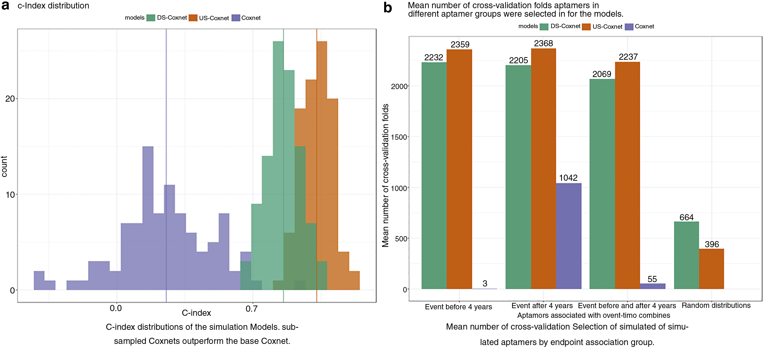
Results for models trained on the 100 simulated data sets, comparing concordance index (a) and number of aptamers selected (b). DS, downsampled; US, upsampled.

Although sampling is an effective approach for mitigating class imbalance in survival modeling, there are a few potential pitfalls. Calculation of AUC, sensitivity, and specificity ignores individuals who were censored before 4 years. This approach may reduce the sample size of the data set being investigated, particularly if there is heavy censoring before the classification time point. In addition, the underlying survival probabilities derived from the final model will likely not represent the probabilities for the entire cohort, given that sampling modifies the prevalence of the disease in the population. Recalibration of the model probabilities from sampling to represent the prevalence in the entire cohort warrants further investigation.

Another item for future exploration is how “class imbalance” is defined for survival models. Because the time to event is incorporated in model development, it is possible that the number of events can become quite small before the sensitivity and specificity metrics are heavily impacted, although this potential effect is currently unknown.

In addition to sampling, there are other methods for handling class imbalance that could be incorporated into survival models, such as case-weighting and SMOTE, which is considered for future study.⁴⁶ Ideally, this article can continue a discussion among scientists on the combination of basic machine learning elements with traditional statistical modeling approaches, particularly in the arena of survival analysis.

Conclusion

Often in survival analysis, class imbalance is a major issue, wherein the number of individuals without a disease (or event) far outnumbers those with the disease within a certain time frame. This imbalance may result in individuals with disease and time to disease being predicted incorrectly. Sampling in time-to-event data can mitigate this issue by balancing the number of individuals in the minority and majority class, thus improving the detection and selection of features related to individuals in the minority class as well as their estimated impact on risk of the disease or event occurring.

Footnotes

Acknowledgments

We thank Dr. Robert K. DeLisle, the Bioinformatics team at SomaLogic, Inc., Dr. Rachel Ostroff and Dr. Steve Williams at SomaLogic, Inc. SOMAmer and SOMAscan are registered trademarks of SomaLogic, Inc. Furthermore, this study would not have been possible without help from researchers and participants in the HUNT3 study.

Authors' Contributions

Y.H., G.D., M.A.H., and L.E.A. conceived the project. Y.H. and M.A.H. provided expertise on survival analysis techniques. Y.H. performed background literature research and M.A.H. provided background on the data used. L.E.A. developed the functions needed for analysis with input from G.D. and Y.H. G.D. performed the analysis required for the research, with input from M.A.H., L.E.A., and Y.H. G.D., Y.H., M.A.H., and L.E.A. cowrote the article. All authors reviewed and approved the final article. The article has been submitted solely to this journal and is not published, in press, or submitted elsewhere.

Authors Disclosure Statement

Y.H., G.D., M.A.H., and L.E.A. are employees of SomaLogic, Inc.

Funding Information

The authors received no specific funding for this work.

Supplementary Material

Abbreviations Used

References

Sanchis-Gomar

, Perez-Quilis

, Leischik

, et al. Epidemiology of coronary heart disease and acute coronary syndrome. Ann Transl Med. 2016; 4:256.

Watkins

, Farrall

. Genetic susceptibility to coronary artery disease: from promise to progress. Nat Rev Genet. 2006; 7:163.

Ganz

, Heidecker

, Hveem

, et al. Development and validation of a protein-based risk score for cardiovascular outcomes among patients with stable coronary heart disease. JAMA. 2016; 315:2532–2541.

Gold

, Ayers

, Bertino

, et al. Aptamer-based multiplexed proteomic technology for biomarker discovery. PLoS One. 2010; 5:e15004.

George

, Seals

, Aban

. Survival analysis and regression models. J Nucl Cardiol. 2014; 21:686–694.

Wang

, Li

, Reddy

. Machine learning for survival analysis: a survey. ACM Comput Surv. 2019; 51:110:3–110:36.

Harrell Jr. FE. Regression Modeling Strategies: With Applications to Linear Models, Logistic and Ordinal Regression, and Survival Analysis, 2nd ed. New York, NY: Springer. 2015.

Vittinghoff E, Glidden DV, Shiboski SC, et al. Regression Methods in Biostatistics: Linear, Logistic, Survival, and Repeated Measures Models, 2nd ed. New York, NY: Springer. 2012.

Hosmer DW. Jr., Lemeshow S, May S. Applied Survival Analysis: Regression Modeling of Time-to-Event Data, 2nd ed. Hoboken, NJ: Wiley. 2008.

10.

Kuhn M, Johnson K. Applied Predictive Modeling. New York, NY: Springer. 2016.

11.

Fawcett

, Provost

. Adaptive fraud detection. Data Min Knowl Discov. 1997; 1:291–316.

12.

Provost F, Fawcett T. Analysis and visualization of classifier performance: comparison under imprecise class and cost distributions. Proceedings of the Third International Conference on Knowledge Discovery and Data Mining (KDD-97). August 14–17. Newport Beach, CA. AAAI Press; 1997. Volume 1. pp. 43–48.

13.

Mladenic

, Grobelnik

Feature selection for unbalanced class distribution and naive Bayes. Proceedings of the Sixteenth International Conference on Machine Learning. June 27–30. Bled, Slovenia. San Francisco, CA: Morgan Kaufmann Publishers, Inc.; 1999. Volume 1. pp. 258–267.

14.

Kubat

, Holte

, Matwin

. Learning when negative examples abound. In: Machine Learning: ECML-97. ECML 1997. Lecture Notes in Computer Science (Lecture Notes in Artificial Intelligence), vol. 1224. (van Someren M, Widmer G; eds). Springer, Berlin, Heidelberg. 1997; pp. 146–153.

15.

Batuwita

, Palade

A new performance measure for class imbalance learning. Application to Bioinformatics Problems. IEEE Xplore, 2009 International Conference on Machine Learning and Applications. December 13–15. Miami Beach, FL. Washington, DC: IEEE; 2009. pp. 545–550.

16.

Boulesteix

A-L

, Janitza

, Kruppa

, et al. Overview of random forest methodology and practical guidance with emphasis on computational biology and bioinformatics. WIREs Data Min Knowl Discov. 2012; 2:493–507.

17.

Liu

T-Y.

EasyEnsemble and feature selection for imbalance data sets. IEEE Xplore, 2009 International Joint Conference on Bioinformatics, Systems Biology and Intelligent Computing. August 3–5. Shanghai, China. Washington, DC: IEEE; 2009. pp. 517–520.

18.

Kotsiantis

, Kanellopoulos

, Pintelas

. Handling imbalanced datasets: a review. GESTS Int Trans Comput Sci Eng. 2006; 30:25–36.

19.

Visa S, Ralescu A. Issues in mining imbalanced data sets—A review paper. Proceedings of the Sixteen Midwest Artificial Intelligence and Cognitive Science Conference (MAICS-2005). April 16–17. Dayton, OH. 2005. Volume 1. pp. 67–73.

20.

Kubat

, Matwin

Addressing the curse of imbalanced training sets: one sided selection. Proceedings of the Fourteenth International Conference on Machine Learning. July 8–12, 1997. Nashville, TN. San Francisco, CA: Morgan Kaufmann Publishers Inc.; 1997. pp. 179–186.

21.

Pazzani

, Merz

, Murphy

, et al. Reducing misclassification costs. Proceedings of the Eleventh International Conference on Machine Learning. July 10–13. New Brunswick, NJ. San Francisco, CA: Morgan Kaufmann Publishers, Inc.; 1994, 217–225.

22.

Japkowicz

. The class imbalance problem: significance and strategies. Proceedings of the 2000 International Conference on Artificial Intelligence (IC-AI’2000): Special Track on Inductive

Learning

. June 26–29, 2000. Las Vegas

. 2000. pp. 111–117.

23.

Chawla

Data mining for imbalanced datasets: an overview. Data Min Knowl Discov Handbook. 2006; 5:853–871.

24.

Beretta

, Santaniello

, Cappiello

, et al. Development of a five-year mortality model in systemic sclerosis patients by different analytical approaches. Clin Exp Rheumatol. 2010; 28:S18.

25.

Chawla

, Japkowicz

, Kotcz

, et al. special issue on learning from imbalanced data sets. SIGKDD Explor. 2004; 6:1–6.

26.

Pavlou

, Ambler

, Seaman

, et al. How to develop a more accurate risk prediction model when there are few events. BMJ. 2015; 351:h3868.

27.

Min

, Lee

, Yoon

. Deep learning in bioinformatics. Brief Bioinform. 2017; 18:851–869.

28.

Cox

Regression models and life-tables. JRSSB. 1972; 34:187–220.

29.

Zou

, Hastic

. Regularization and variable selection via the elastic net. JRSSB. 2005; 67:301–320.

30.

Simon

, Friedman

, Hastie

, et al. Regularization paths for Cox's proportional hazards models via coordinate descent. J Stat Softw. 2011; 39:1–13.

31.

Tibshirani

The lasso method for variable selection in the cox model. Stat Med. 1997; 16:385–395.

32.

Krokstad

, Langhammer

, Hveem

, et al. Cohort profile: the HUNT Study, Norway. Int J Epidemiol. 2013; 42:968–977.

33.

Rohloff

, Gelinas

, Jarvis

, et al. Nucleic acid ligands with protein-like side chains: modified aptamers and their use as diagnostic and therapeutic agents. Mol Ther Nucleic Acids. 2014; 3:e201.

34.

Kaplan

, Meier

. Nonparametric estimation from incomplete observations. J Am Stat Assoc. 1958; 53:457–481.

35.

Friedman

, Hastie

, Tibshirani

. glmnet: Lasso and elastic-net regularized generalized linear models. Available at https://CRAN.R-project.org/package=glmnet (accessed July 1, 2019).

36.

R Core Team. R: A Language and Environment for Statistical Computing. Vienna, Austria: R Foundation for Statistical Computing. 2018. Available at https://www.R-project.org (accessed July 1, 2019).

37.

RStudio Team. RStudio: Integrated Development Environment for R. Boston, MA: RStudio, Inc. 2016. Available at http://www.rstudio.com (accessed July 1, 2019).

38.

Jake

, Krzywinski

, Altman

. Points of significance: model selection and overfitting. Nat Methods. 2016; 13:703–704.

39.

Benjamini

, Hochberg

. Controlling the false discovery rate: A practical and powerful approach to multiple testing. J R Stat Soc B. 1995; 57:289–300.

40.

Harrell

, Lee

, Mark

. Multivariable prognostic models: issues in developing models, evaluating assumptions and adequacy, and measuring and reducing errors. Stat Med. 1996; 15:361–387.

41.

Harrell

. Jr., Califf

, Pryor

, et al. Evaluating the yield of medical tests. J Am Med Assoc. 1982; 247:2543–2546.

42.

Harrell

. Jr., Lee

, Califf

, et al. Regression modeling strategies for improved prognostic prediction. Stat Med. 1984; 3:143–152.

43.

Harrell

, Lee

, Mark

. Tutorial in biostatistics: multivariable prognostic models: issues in developing models, evaluating assumptions and adequacy, and measuring and reducing errors. Stat Med. 1996; 15:361–387.

44.

Hastie

, Tibshirani

, Friedman

. The Elements of Statistical Learning: Data

Mining

, Inference and

Prediction

, 2nd ed. New York

: Springer. 2009.

45.

Cortes

, Vapnik

. Support-vector networks. Mach Learn. 1995; 20:273–297.

46.

Chawla

, Bowyer

, Hall

, et al. SMOTE: synthetic minority over-sampling technique. J Artif Intell Res. 2002; 16:321–357.

Supplementary Material

Please find the following supplemental material available below.

For Open Access articles published under a Creative Commons License, all supplemental material carries the same license as the article it is associated with.

For non-Open Access articles published, all supplemental material carries a non-exclusive license, and permission requests for re-use of supplemental material or any part of supplemental material shall be sent directly to the copyright owner as specified in the copyright notice associated with the article.

0.26 MB

0.08 MB

0.03 MB

0.00 MB

Balanced Event Prediction Through Sampled Survival Analysis

Abstract

Introduction

Materials and Methods

Data set

Cox elastic net models

Sampling methods

Data subsetting

Workflow

Results

Simulation results

Analysis of HUNT3 research study data

Model results and comparison

Threshold investigation

Discussion

Conclusion

Footnotes

Acknowledgments

Authors' Contributions

Authors Disclosure Statement

Funding Information

Supplementary Material

Abbreviations Used

References

Supplementary Material