Aviation Benefits from Satellite Navigation

Abstract

Abstract

The global navigation satellite systems (GNSS) benefit aviation by enabling aircraft to fly direct from departure to destination using the most fuel-efficient routes and to navigate complicated terrain at low altitude. Satellite navigation provides the flexibility to design new procedures that enable aircraft to fly closer together to increase the arrival and departure rates and fly continuous climb and descent operations to minimize fuel consumption, noise, and carbon emissions. Using the language of the aviation community, GNSS enables performance-based navigation, which consists of area navigation (RNAV) and required navigation performance (RNP). Both RNAV and RNP enable unrestricted point-to-point flight paths. RNP differs from RNAV, because it also provides a monitoring and alerting function to warn the pilot when a correction is required, enabling aircraft to fly tighter flight paths. GNSS is the only navigation source approved for RNP operations. This article introduces these new capabilities, and the GNSS augmentations needed to ensure that the evolution of air navigation remains safe.

Introduction

The global navigation satellite systems (GNSS) serve an enormous breadth of users in the air, on the ground, at sea, and in space. These widespread users enjoy 5 m location accuracy worldwide, 24 h/day, in all weather. If better accuracy is required, differential techniques are available to provide decimeter or even centimeter accuracy.

Figures 1 and 2 show the satellites that enable this global utility. Specifically, Figure 1 shows the satellites from the global positioning system (GPS) that are on orbit in mid-2014. The GPS satellites are in medium earth orbit (MEO), and seven satellites in geostationary orbit (GEO) augment this core constellation by broadcasting safety information for aviation. GPS has been the mainstay of GNSS, but new constellations are being deployed by China and Europe, and Russia has rejuvenated their GLONASS system. Figure 2 shows all of the GNSS satellites that are on orbit in mid-2014. As shown, this superset occupies MEO, GEO, and inclined geosynchronous orbits.

Fig. 1.

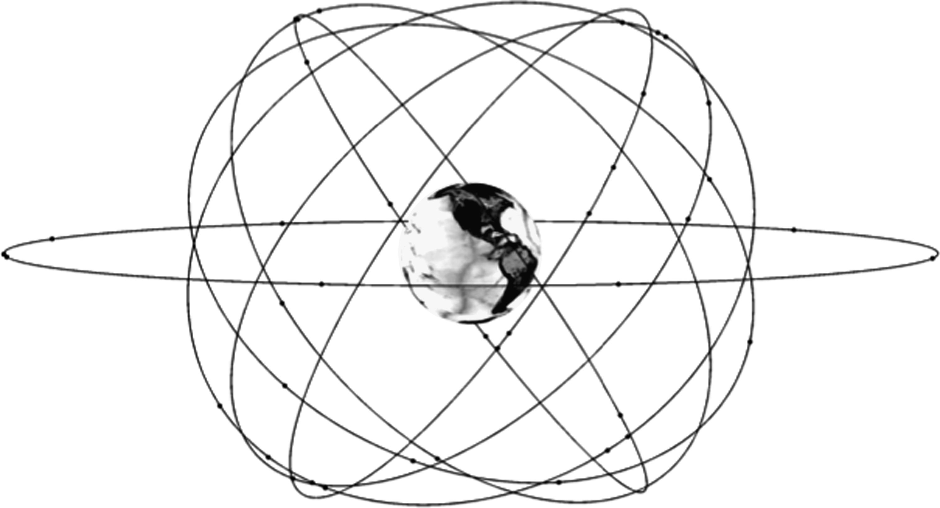
Global positioning system (GPS) satellites on orbit in May 2014. Today, GPS has approximately 32 satellites in medium earth orbit (MEO). Also shown, seven satellites in geostationary orbit (GEO) augment GPS; they broadcast real-time error bounds to support aviation use. (Courtesy of Tyler Reid)

Fig. 2.

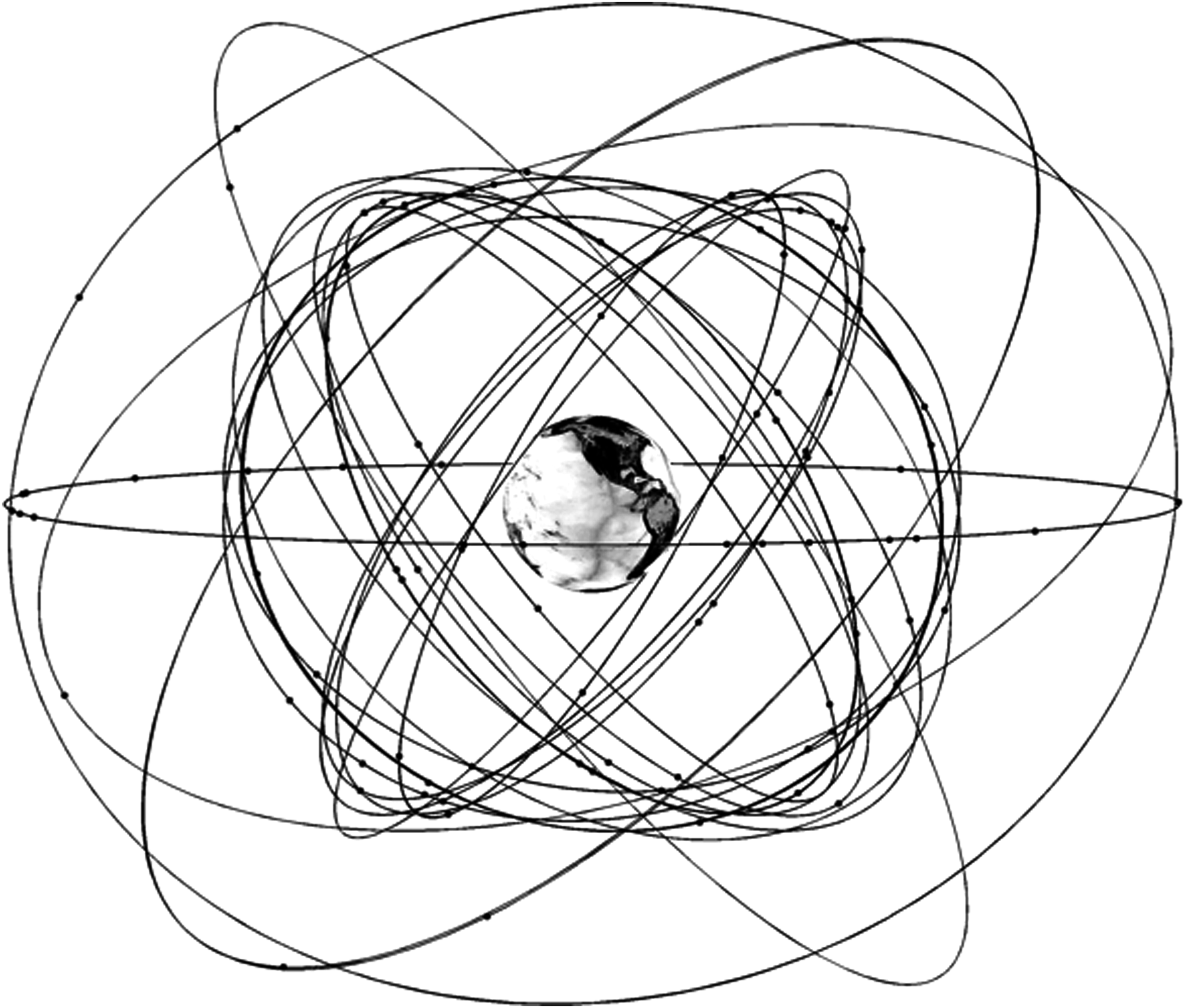
Global navigation satellite system (GNSS) satellites on orbit in May 2014. This figure includes satellites from GPS, GLONASS (Russia), Beidou (China), Galileo (Europe), Quasi-zenith Satellite System (QZSS, Japan), and the Indian Regional Navigation Satellite System (IRNSS). As shown, these constellations include satellites in MEO, GEO, and inclined geosynchronous orbits. (Courtesy of Tyler Reid)

GNSS is passive; the signal travels from the satellites to the users, while the user does not radiate any signals. These satellite signals are in the L band of the radio spectrum (1.0–2.0 GHz), and are carefully crafted to enable very accurate time-of-arrival (ToA) measurements by the user. With four such ToA measurements, users can estimate their latitude, longitude, altitude, and time offset from the satellite system time. In short, four (or more) equations are used to estimate the four unknowns. GNSS solves for the user time offset relative to the GNSS system time, which in turn is connected to the coordinated universal time (UTC). For this reason, GNSS is called a space-based position navigation and time (PNT) system.

Figure 3 shows the basic operation associated with one of the GNSS satellites. Each satellite broadcasts a carefully crafted signal that enables precise ranging measurements by the receiving equipment. The signal from each GNSS satellite has two ingredients. First, each satellite sends a unique code that creates sharp radio marks that the receiver can readily distinguish from background noise and the signals from other satellites. This code has special correlation properties that enable the user equipment to measure its ToA to within a few billionths of a second. Second, each satellite superposes needed data on top of the codes using a so-called navigation message. These data include the satellite location and the signal time-of-transmission. Together, these two ingredients allow the receiver to precisely measure the arrival time of the signal from a few GNSS satellites.

Fig. 3.

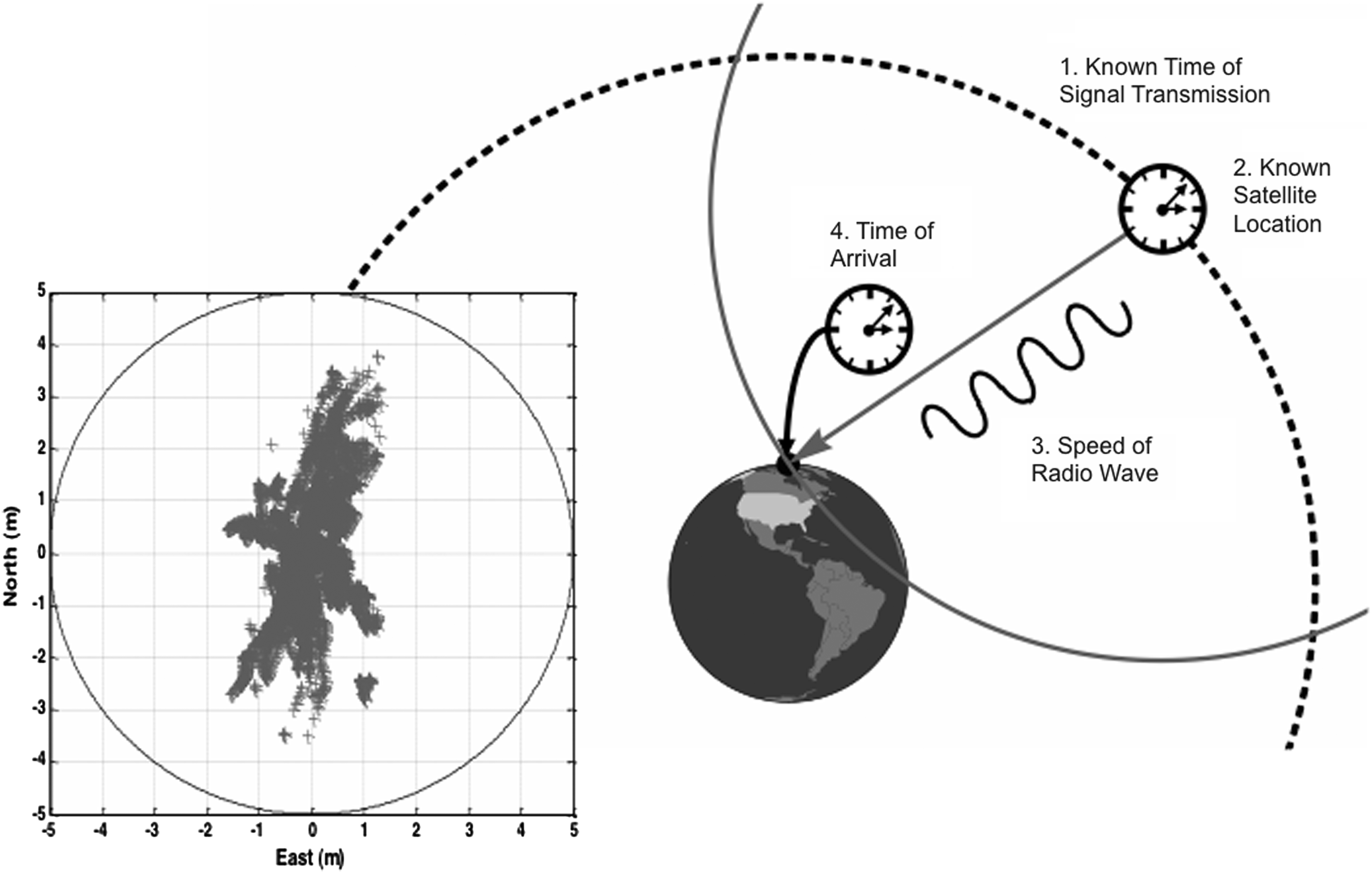
Basic operation of a GNSS satellite showing the key ingredients of a pseudorange measurement. These include (1) known transmission time of a satellite-unique spread-spectrum code, (2) known location of the satellite at the transmission time, (3) known propagation speed of the radio wave, and (4) accurate measurement of signal time-of-arrival. The typical accuracy of a GNSS receiver is shown in the scatter plot.

The GNSS signal travels at a speed that is very close to the speed of light, but it passes through the ionosphere and troposphere on its trip from orbit to the user, and these interventions slightly slow the wave. These deviations in speed are reasonably well modeled, and can be corrected for, as will be explained later.

The user equipment (i.e., GNSS receiver) measures the ToA of the signal by correlating the satellite codes with replica codes stored in the receiver. As mentioned above, the satellite provides the transmission time and location by broadcasting a navigation message in addition to the ranging code. The user subtracts the transmission time from the arrival time, and this time difference is shown below as t_rcv – t_tmt. \documentclass{aastex}\usepackage{amsbsy}\usepackage{amsfonts}\usepackage{amssymb}\usepackage{bm}\usepackage{mathrsfs}\usepackage{pifont}\usepackage{stmaryrd}\usepackage{textcomp}\usepackage{portland, xspace}\usepackage{amsmath, amsxtra}\pagestyle{empty}\DeclareMathSizes{10}{9}{7}{6}\begin{document} \begin{align*} & \rho = { \rm c} ( { \rm t}_{{ \rm rcv}} - { \rm t}_{{ \rm tmt}} ) \\& \ = { \rm range} + { \rm c b}_{{ \rm rcv}} \\& \ = \sqrt{ ( { \rm x}_{{ \rm rcv}} - { \rm x}^{ ( { \rm sat} ) } ) ^2 + ( { \rm y}_{{ \rm rcv}} - { \rm y}^{ ( { \rm sat} ) } ) ^2 + ( { \rm z}_{{ \rm rcv}} - { \rm z}^{ ( { \rm sat} ) } ) ^2} + { \rm c} { \rm b}_{{ \rm rcv}} \\& { \rm t}_{{ \rm rcv}} = \hbox{arrival time measured by receiver} \\& { \rm t}_{{ \rm tmt}} = \hbox{broadcast time marked by satellite} \\& \hbox{\rm range} = \hbox{range from satellite to receiver} \\& { \rm c} = \hbox{speed of light} \\& { \rm b}_{{ \rm rcv}} = \hbox{receiver clock time difference from GNSS time} \\& \{ { \rm x}_{{ \rm rcv}} , { \rm y}_{{ \rm rcv}} , { \rm z}_{{ \rm rcv}} \} \hbox{user location} \\& \{ { \rm x}^{ ( { \rm sat} ) } , { \rm y}^{ ( { \rm sat} ) } , { \rm z}^{ ( { \rm sat} ) } \} \hbox{satellite location}\end{align*} \end{document}

When converted to distance, this time difference is known as the pseudorange (ρ), because it is equal to the geometric range from the satellite to the user plus an added bias (b_rcv) due to the time difference between the receiver clock and GNSS time.

Each pseudorange measurement is sensitive to the receiver location (x_rcv, y_rcv, z_rcv) and receiver clock offset, b_rcv. These four quantities (x_rcv, y_rcv, z_rcv, b_rcv) are known as the estimanda or the user state. The other variables in this equation are reasonably well known. Recall that the satellite broadcasts its location as part of the navigation message. Thus, four such pseudorange measurements are needed for the estimation of the four-dimensional user state. While four satellites are certainly necessary to estimate the user state, four satellites may not be sufficient. The satellites must have good geometry relative to each other; they must be spread across the sky and not bunched together or co-planar.

Figure 3 shows the typical performance of a GNSS receiver in 2013. A two-dimensional scatter plot characterizes the performance of the receiver. The reported locations are scattered around the origin (0, 0), where the receiver is truly located. As shown, the errors are generally smaller than 5 m. As mentioned earlier, and detailed later, differential navigation relative to a reference receiver at a known location can improve this performance to yield decimeter or centimeter accuracies. By the way, the N–S orientation of the scatter in Figure 3 is specific to this data set, and not a general feature of satellite navigation.

The data set shown in Figure 3 is based on the GPS, which is presently the most-used satellite constellation within the GNSS. GPS was originally developed by the U.S. Department of Defense in the 1970s. At that time, the planners predicted that GPS would serve a total of 40,000 military users with some ancillary civil use. Today, the civil community has shipped over 3 billion GPS receivers. The civilian tail now wags the GPS dog, and the civil aviation community has already benefited from a growing set of GPS applications that are directed at increasing efficiency, saving fuel, and reducing the environmental impact of aviation.

As mentioned earlier, GPS is not alone. Russia has rejuvenated their satellite navigation system, called GLONASS, which has 24 satellites as of December 2013. Europe has launched their first prototype satellites for their Galileo system, which will eventually have 24 satellites. China is expanding their regional system, BeiDou, to include global coverage. Japan and India have also launched satellites for regional systems. Figure 2 depicts the current mélange of satellites in this system of systems. In time, these national constellations will comprise a mighty GNSS with over 100 satellites.

The multiplicity of satellites described above will provide geometric diversity with signals coming from almost every overhead direction. Importantly, the new satellites will also provide frequency diversity for civil users. Each new satellite will radiate civil signals at three frequencies rather than the single civil frequency offered before 2010.

Figure 4 shows the spectrum for the new GNSS signals that are coming on line in the next 10 years. All of these signals reside in portions of the radio spectrum that have been set aside for radio navigation satellite systems. Some also reside in bands that have been allocated for aeronautical radio navigation systems (ARNS). As shown, the GPS satellites broadcast at three civil frequencies called L1 (1575.42 MHz), L2 (1227.60 MHz), and L5 (1176.45 MHz). L1 is home to the so-called clear access (C/A) signal; this GPS signal is the basis for the vast majority of civil applications to date. This C/A signal overlays military signals in the same band. L2 also carries a civil signal on the seven most recent GPS satellites. L5 is the home for the third civil signal, and has been included on the four most recent GPS satellites. L5 has a broader spectrum than the civil signals at L1 and L2, and so it is the most robust civil signal.^1–3

Fig. 4.

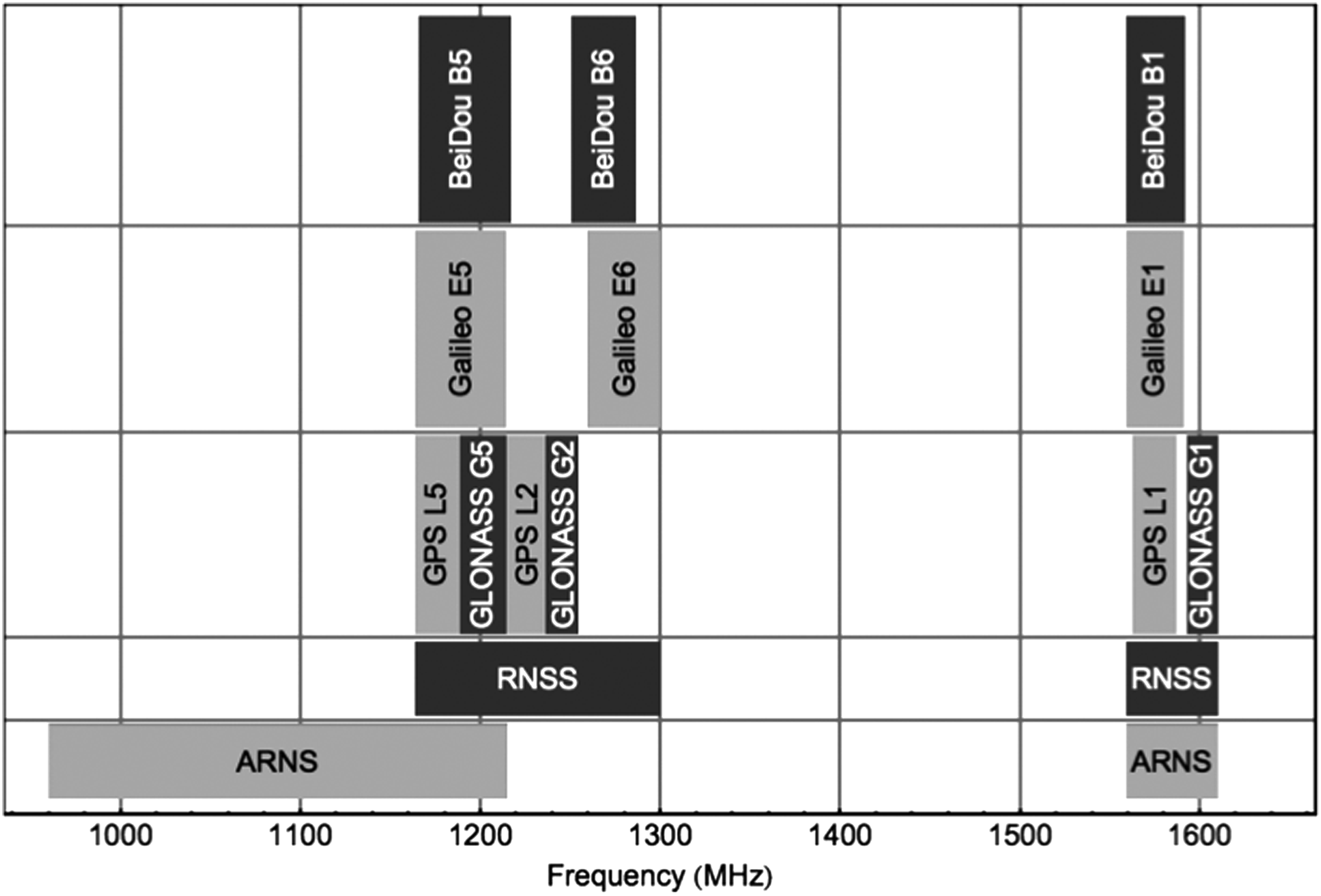
Signal spectra for GPS, Galileo, BeiDou, and GLONASS. From the left, new GPS satellites radiate at L5 (1176.45 MHz), L2 (1227.60 MHz), and L1 (1575.42 MHz).

Taken together, L1, L2, and L5 provide redundancy to combat accidental radio frequency interference (RFI) and a means to remove the dispersive delay due to the ionosphere. Both features are important. RFI is becoming more prevalent in the GPS bands, and the ionosphere is the largest natural source of error. These two challenges will be further described later in this article. L1 and L5 are particularly important to aviation, because they both fall in ARNS portions of the radio spectrum. Thus, they have greater aviation utility, because they enjoy greater institutional protection than L2.

The signals for GLONASS, Galileo, and Compass are also shown in Figure 4. As illustrated, they are not located at exactly the same places as the GPS signals. However, they share the main features: triple-frequency diversity with at least two signals in the ARNS bands surrounding L1 and L5.

As mentioned earlier, GPS user equipment serves a multitude of applications. For example, every new Boeing or Airbus aircraft carries a GPS receiver for navigation in the enroute and terminal area airspace. GPS is also used to guide aircraft while approaching airports. In some cases, it provides the most critical vertical dimension of location down to altitudes of 200 feet. GPS receivers for aviation are expensive, due to the cost associated with the design and testing for such a critical safety application.

At the other cost extreme, most new mobile phones carry GPS/GLONASS receivers that have a bill of materials around $1. These receivers are used to guide our walking and driving lives. They also provide our location automatically to emergency services when we make such a call.

We are now well prepared to engage the body of this article. The Efficiency and Environmental Benefits section focuses on the efficiency and environmental benefits to aviation from GNSS, describing four aviation operations where GNSS enables fuel savings. These operations are based on the area navigation (RNAV) capability of GNSS. The section titled Safety focuses on the safety of air navigation based on GNSS. More specifically, it describes the required navigation performance (RNP) and discusses the technology needed to ensure that human-made faults, space weather, and bad actors (jammers and spoofers) do not endanger aircraft using GNSS for navigation. The Summary section is a brief summary of this article.

Efficiency and Environmental Benefits

As mentioned earlier, satellite navigation will save aviation fuel and reduce the environmental impact of flight. To tell this tale, we begin by discussing a parallel development: the eco-routing of automobiles. Following this ground-based discussion, we turn our attention to the air. In the subsection titled Juneau, Alaska, and Jackson Hole, Wyoming, we discuss the applications of GNSS to the departure and approach to airports in mountainous terrain. In the subsection Optimized Profile Descent, we continue our discussion of approach procedures by describing optimized profile descents (OPDs) that can save fuel and reduce noise pollution. The subsection Tailored Arrivals broadens our interest to the terminal area that surrounds a metropolitan airport (e.g., the New York multiplex or the San Francisco Bay Area with its three major airports). The subsection Optimized Enroute Flight extends our discussion to oceanic paths that adapt to weather conditions on a seasonal, daily, or even hourly basis.

Eco-Routing for Automobiles

Recently, Ford and Hyundai, in partnership with TeleNav and Navtech, have been working to improve the efficiency of automobiles by deploying the so-called eco-routing or “green GPS” navigation systems in their cars. Like other automotive navigation systems, these systems use distance and average speed to calculate the “shortest” route and “fastest” route from point A to point B. However, they also consider additional factors in order to provide the “greenest” or most fuel-efficient route. Some of these eco-factors are

• Stoplights and stop signs: avoid stopping

• Traffic: avoid stop-and-go, idling, and very low speed

• Curves: avoid deceleration and re-acceleration

• Hills: avoid hill-climbing

A study of one such eco-routing navigation system found that taking the greenest route resulted in an average of 10% fuel savings. ⁴ This estimate is conservative, as these savings are as compared to the existing “fastest route” provided by standard navigation systems, which is already significantly more fuel efficient than the average route taken without using a navigation system. Given that highway CO₂ emissions account for 26% of the U.S. total from all sources, eco-routing for all U.S. road trips has the potential to reduce total U.S. CO₂ emissions by 2.6%, an impressive impact for such a simple solution. ⁵

By coincidence, while highway eco-routing has the potential to save 2.6% of U.S. CO₂ emissions, U.S. aviation accounts for only 2.6% of total U.S. CO₂ emissions to begin with. ⁵ Even so, aviation will be one of the most difficult sectors in which to reduce emissions. This intransigence is due to aviation's requirement for fuels with the greatest energy density (joules/kilogram and joules/volume). Thus, as total emissions decline in the future, aviation's contribution will loom larger. As the relative impact of aviation increases, so will the importance of finding effective methods of reducing its growing fraction of global CO₂ emissions.

In the recent history of aviation, innovations in airframe design and propulsion systems have resulted in significant reductions in aircraft fuel consumption. Between 1960 and 2008, the average fuel burn of new aircraft decreased by more than half, thanks to improvements in engine efficiency and aerodynamics, and more efficiently utilized capacity.^6,7 With the recent introduction of the Boeing 787, designed to be 20% more efficient than similar aircraft, this hopeful trend will continue. ⁸

This article does not further consider aerodynamics and propulsion; rather, it focuses on the use of navigation technology to enable more efficient aircraft routes and procedures. In this section, we will explore several of these operational improvements, each of which has been enabled by advanced air navigation systems, primarily GNSS. It is important to note, however, that the efficiency improvements due to navigation and those due to airframe design and propulsion are additive.

Juneau, Alaska, and Jackson Hole, Wyoming

Alaska Airlines was the first airline to routinely employ GPS guidance when approaching airports. Severe weather and landscape increase the need for navigation when approaching or departing from an Alaskan airport. GPS is vital in Alaska, because it provides navigation signals that surround the entire airport, enabling unrestricted RNAV. RNAV enables aircraft to fly directly between any two points rather than flying the less efficient conventional routes between two radio navigation stations on the ground. For example, Alaska Air initiated the use of GPS when flying into the state capital, Juneau. This city is accessible only by air and water, and the air routes require several turns and appreciable consideration of safety.

Figure 5 shows a fuel-efficient path for aircraft departing from or approaching Juneau airport. As shown, this path follows the Gastineau Channel and the aircraft flies northwest to approach Runway 26 at Juneau airport. Cliffs define both sides of this channel, and the Alaskan weather frequently blocks the view of these boundaries. Fortunately, Alaskan Airlines was able to work with the Federal Aviation Administration and The Boeing Company to define the path shown in Figure 5. GPS precise positioning with receiver autonomous integrity monitoring (RAIM), which we will discuss in the section titled Safety, enabled Alaska Airlines to navigate the channel in low visibility. Before this capability, aircraft were compelled to avoid Juneau if the weather ceiling was below 1000 feet or the along-track visibility was less than 2 miles. With GPS-based navigation of the Gastineau Channel, the tolerable weather ceiling was dropped to 337 feet and the along-track visibility shortened to 1 mile.

Fig. 5.

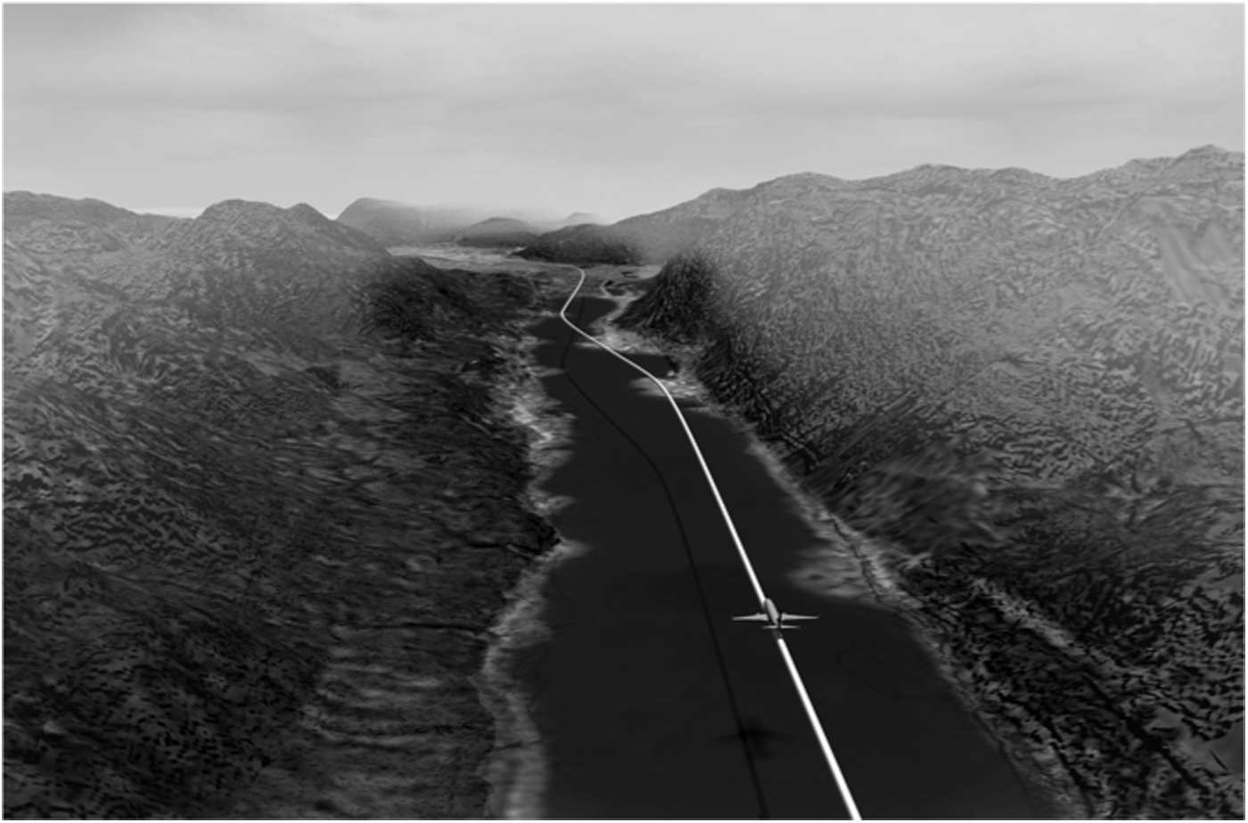
Departures and arrivals from Juneau Airport (JNU) using the Gastineau Channel. The left turn at the far end of the channel, close to the airport, requires an area navigation (RNAV) capability. Such a path bend cannot be supported with a line-of-sight radio beam from the ground. (Courtesy of BridgeNet International)

In 1996, Alaska Airlines began to use the Gastineau Channel in earnest. By 2011, Alaska Airlines flew 5,683 arrivals through the narrow Gastineau Channel with the assistance of GPS navigation. Of these flights, 831 were saves, or flights that would have been canceled or diverted due to weather if they had not been equipped with GPS. Each year, Alaska Airlines attributes a savings of approximately $1 million to this GPS-based capability in Juneau.

Today, Alaska Airlines uses GPS to support navigation into 30 airports in Alaska and in the continental United States. They operate a fleet of 117 Boeing 737s equipped with this capability, and their sister airline Horizon Air operates similarly capable Bombardier Q400 turboprops. According to Alaska Air, the airline flew 12,700 approach and departure procedures in 2011, avoiding the diversion of 1,545 flights through the use of GPS navigation. In that year, the airline used GPS to help reduce fuel use by 210,000 gallons and save more than $15–$19 million across their entire fleet and operations.

Jackson Hole, Wyoming, also has a unique airport that benefits from GPS. Figure 6 shows the approach path from above. The airport (JAC) is located at the bottom left of the figure. As shown, the conventional landing route requires two straight line segments based on the limitations of conventional ground-based radio navigation systems. The first segment flies westward, and the second segment flies southward to the airport. The new path uses RNAV waypoints for a curved path that avoids the sharp turn and the noise-sensitive area near Grand Teton National Park. This new path is shorter by 14 miles and 3 min of flight time.

Fig. 6.

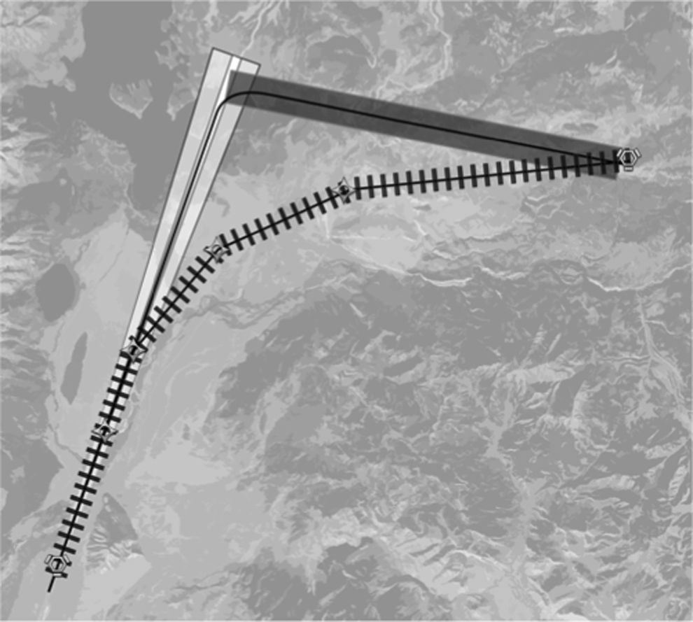
Arrival to Jackson Hole (JAC) Airport using GPS-enabled RNAV. The RNAV path is curved and shorter, and avoids the main attractions of the Grand Teton National Park. (Courtesy of BridgeNet International)

Optimized Profile Descent

In the cases of Juneau and Jackson Hole, the approach designers optimized the horizontal ground track. However, it is also possible to fly more efficient vertical profiles using an OPD, enabling qualified aircraft to reduce fuel, noise, and carbon emissions. Currently, standard terminal arrivals use a series of mandatory altitudes along the arrival route that gradually step the aircraft down to the airport. The advantage of this step-down design is that it is easy to standardize and minimizes the volume of protected airspace around the airport. In terms of fuel efficiency, time, and noise pollution, however, the step-down approach is not ideal because aircraft use higher power settings to maintain level flight.

An ideal OPD is a continuous descent operation, where the aircraft descends all the way from cruise altitude to the runway in a smooth glide trajectory using low power, saving time and fuel and reducing noise and emissions (see Fig. 7). Some of these descending aircraft may be idling, while some may need slightly more power to enable anti-icing. These OPDs are published procedures, and so the controller can clear the aircraft to fly the OPD. When cleared, an aircraft can descend safely from near-cruise altitude to near the runway, at near-idle thrust.

Fig. 7.

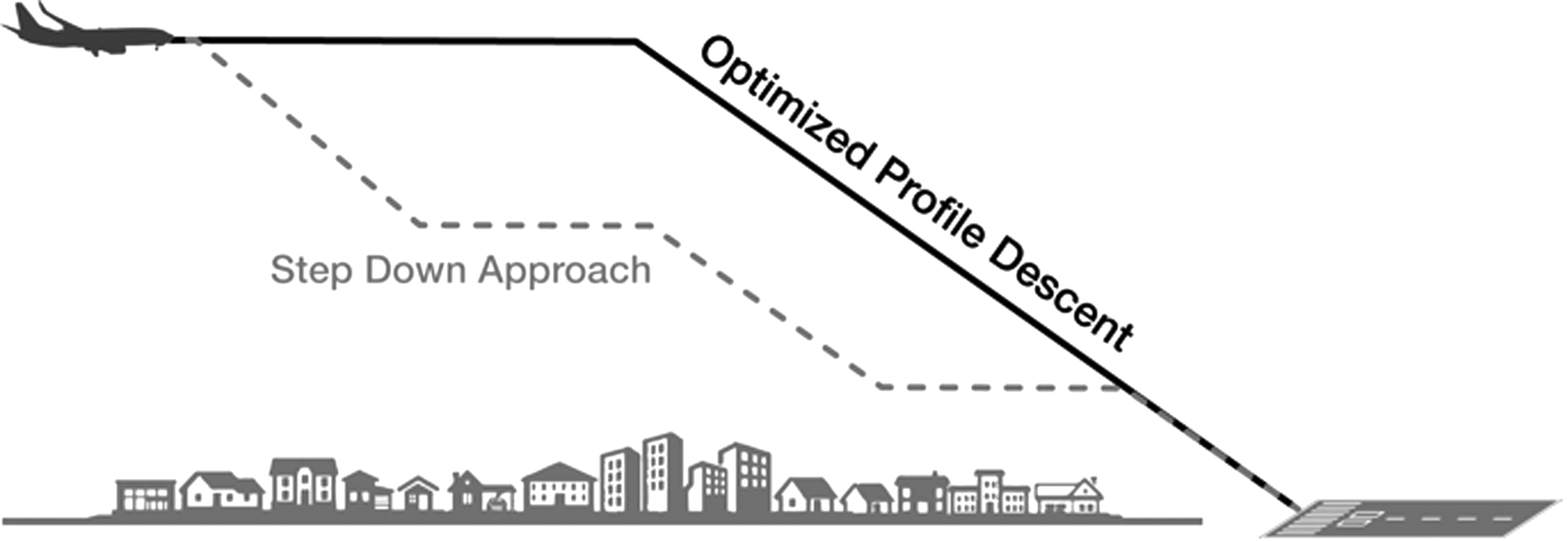
Optimized profile descents (OPD) in contrast to step-down approaches (drive and dive). OPD offers a close approximation to the optimal idle-thrust glide slope and can save hundreds of kilograms of fuel per flight. (Courtesy of BridgeNet International)

The first OPD flight tests were conducted roughly a decade ago at Louisville International Airport (SDF). The SDF descent resulted in average fuel savings of approximately 200 kg per approach of the B737-300 test aircraft. Peak noise levels were also significantly reduced. ⁹

In December 2007, Los Angeles International Airport (LAX) implemented the first publicly charted OPD. Across the LAX fleet, each aircraft using this fully operational OPD saves an average of 25 gallons (76 kg) and 200 kg of CO₂ emissions per approach. Overall, the OPD at LAX saves approximately 2 million gallons (6 million kg) of fuel each year and reduces annual CO₂ emissions by 19 million kg. The OPD also saves time, shaving 44 s off the average flight time, and has decreased the ground noise around LAX. ¹⁰

Significant fuel savings have been demonstrated in flight trials at other airports as well. For example, OPD flight tests with B757s and B737-800s into Miami International Airport (MIA) showed an average savings of 49 gallons (150 kg) of fuel per approach, and tests of B767s into Hartsfield–Jackson Atlanta International Airport (ATL) demonstrated an average savings of 37 gallons (113 kg) per flight. ¹¹

OPD savings depend on the efficiency of the OPD trajectory, the inefficiency of the conventional approach, the type of aircraft, and the weather. At present, the FAA is developing new merging and spacing tools for the controllers to sequence the aircraft on to the OPDs. These improved tools will enable controllers to meter aircraft hundreds of miles away from the aircraft and in the terminal area.

Tailored Arrivals

If you have a smartphone or tablet, you may have played Flight Control, the surprisingly addictive game where the goal is to direct planes to their assigned runways while avoiding potential conflicts. It starts out easy, with one plane and then two, and in these low-traffic conditions, you are free to choose any path you want. But as the game progresses, and the number of planes on the screen increases, your choice of flight paths becomes much more restricted. If your strategy for the game is similar to ours, when the difficulty increases, you end up playing it safe, creating an orderly queue of aircraft for each runway, and directing each new plane to the back of the line, even if that means tracing out a much longer path than you might have otherwise.

While the job of real-world air traffic controllers requires much more skill than this simple game, the basic strategy is similar. When the sky is clear, fuel-efficient flight paths are great. When there is traffic in the sky, avoiding conflicts becomes the number one priority, to the detriment of fuel efficiency. Of course, these priorities are exactly as they should be: safety trumps fuel efficiency.

Unfortunately, this means that the potential benefits of optimized routing often go unrealized in real-world circumstances. Fortunately, fuel efficiency and safety need not always be in opposition. Using tailored arrivals, we can simultaneously increase fuel efficiency while decreasing air traffic controller workload and improving safety.

Tailored arrivals allow for customized arrival pathways for individual flights based on real-time air traffic conditions. The basic concept is this: accurately measure the position and velocity of each aircraft continuously. Use that information, along with real-time weather data, to accurately predict where each aircraft will be in the future. Optimize all of the arrival (and departure) paths together, simultaneously reducing fuel consumption and flight time for each flight while maintaining separation and avoiding conflicts. An example is depicted in Figure 8.

Fig. 8.

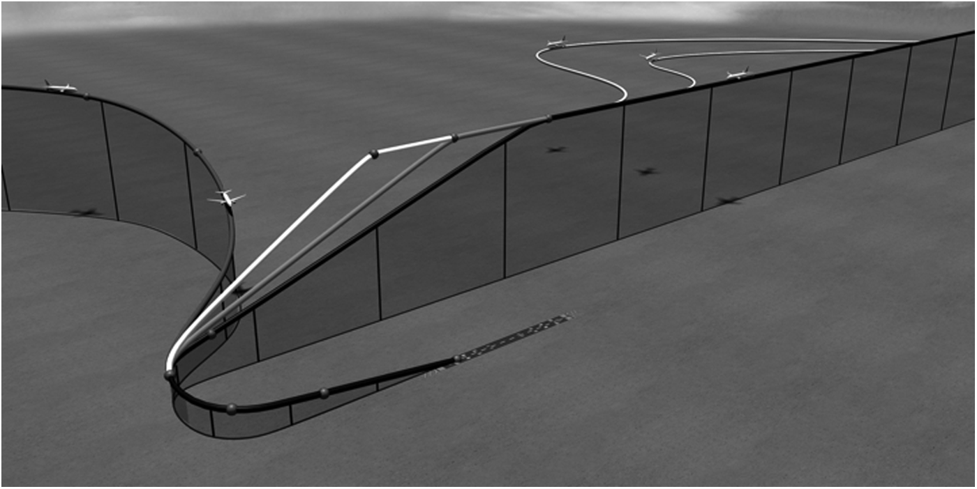
Tailored arrivals. These aircraft are engaging in advanced terminal arrival procedures. Each of the aircraft arriving from the right uses glide slope angles that minimize fuel use for their aircraft. Also, the aircraft arriving from the left joins the approach pattern shared with the first three aircraft, which have left an opening in the pattern in anticipation. (Courtesy of BridgeNet International)

Here is how it plays out in practice: the incoming aircraft downlinks its data to air traffic control, which use a computer program such as NASA's En Route Descent Advisor to generate an optimal descent trajectory. This computed trajectory considers the state of the aircraft, the predicted trajectories of other aircraft in the airspace, and the weather. This optimal approach pathway is then uplinked to the aircraft and loaded into the flight management system. While the technological capabilities to design and fly these tailored arrivals are not yet widely operational (on the ground or in the air), there have been several promising tests of the concept.

In 2006, United collaborated with the FAA to test the concept on 40 flights from Honolulu to San Francisco (SFO) in various traffic conditions. Under light-traffic conditions, the tailored arrival with an OPD approach into SFO resulted in average fuel savings of 110 kg, similar to the standard OPD trials described above. Under heavy-traffic conditions, average fuel savings rose to 1,460 kg per approach. This dramatic increase in savings can be explained by the inefficiencies of the conventional heavy-traffic approach into SFO, which includes a 30 nm path-stretch at low altitude. ¹² Traditionally, during heavy traffic, any given flight is looped around to the back of the line. Tailored arrivals allow the flight to be feathered right into the middle of the queue as the aircraft continues to travel along its own most efficient approach trajectory. In summary, the SFO trials demonstrate that tailored arrivals can save more fuel in heavy traffic, because conventional heavy-traffic approaches are often much less efficient than the low-traffic approaches. (Note: The cited benefits are after a 25% penalty based on the assumption that in heavy-traffic conditions, some upstream path-stretching will still be required to adequately coordinate arrival times. The actual savings of a truly ideal approach compared to a conventional heavy-traffic approach would be 1,896 kg.)

In a later phase of testing at SFO, four airlines testing tailored arrivals at SFO saved more than 500,000 kg of fuel over the course of a year. Tests of tailored arrivals in Melbourne and Sydney found an average savings of 100–200 kg of fuel per approach, and later trials in Brisbane saved 200,000 kg of fuel and 650,000 kg of CO₂ emissions over the course of a year.^13,14

Optimized Enroute Flight

GNSS also enables advanced procedures for aircraft in enroute or oceanic flight by considering distance, winds, and convective weather. While eco-routing on the road is limited to choosing the best route using existing highways, eco-routing in the air can go one step further, choosing efficient routes that break free from the traditional highways in the sky. Assisted by GNSS, aircraft can now safely fly routes that deviate from the fixed air traffic service (ATS) routes, realizing significant fuel savings and emissions reductions, while simultaneously saving time and reducing conflicts. Figure 9 shows a hierarchy of such capabilities.

Fig. 9.

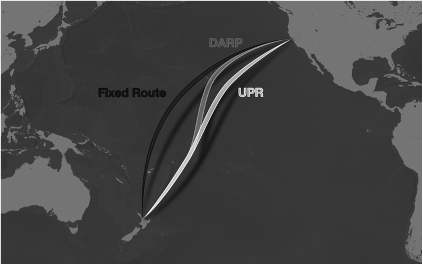
Three enroute track protocols: (1) fixed tracks, (2) user preferred routes (UPR), and (3) dynamic airborne reroute procedures (DARP). (Courtesy of BridgeNet International)

Flexible track systems

The simplest form of optimized routing in the sky is the flexible track system. Operators design and fly an optimized track between a pair of cities, a route that is predicted to be more efficient than the traditional ATS route based on general meteorological forecasts and a representative aircraft performance model. This optimized track becomes the route for all flights between the paired cities, and is updated seasonally.

Demonstrating the potential inefficiency of the old fixed tracks, and the potential savings that can be realized by switching to flexible track systems, a trial of 592 Emirates Airlines flights between Dubai and Melbourne/Sydney resulted in an average fuel savings of 1,000 kg per flight, and an average of 6 min saved per flight. ¹⁵

User-preferred routes (UPR)

User-preferred routes are similar to flexible track systems, but they are updated for individual flights based on short-term, specific forecasting. They consider the specifications of the particular aircraft that will be flying (e.g., B737 and A380), and the most up-to-date information about the wind and convective weather for the specific date and time the aircraft will be flying (e.g., October 17, 2013, at 09:25 PST). UPRs optimize the track for a single flight, which can be significantly different from the optimal track for the same flight flown by a different aircraft at a different time on the same day.

As a result of this flight-specific optimization, UPRs have even greater fuel-saving potential than flexible-track systems. In UPR flight tests between New Zealand, and Japan and China, Air New Zealand obtained a savings of 616 kg of fuel savings per flight, adding up to savings of 1.09 million kg of fuel and 3.44 million kg of CO₂ per year. ¹⁶ In a model of 15 million flights over the course of a year in the United States national airspace, optimizing for wind resulted in an average fuel savings of 95 kg per flight, and an estimated time saving of 2.7 min per flight. In addition, there was an estimated 29% reduction in conflicts as a result of route diversification, meaning that UPRs could potentially improve safety in addition to fuel economy. ¹⁷

Dynamic airborne reroute procedure (DARP)

Dynamic airborne reroute procedures are similar to FTS and UPR, but they can be updated during the flight, based on short-term, specific forecasting. DARP flights begin with a UPR route, but update this route en-route based on the current weather. Based on its DARP flight tests between Auckland (AKL) and SFO, Air New Zealand reports that 58% of their AKL–SFO flights have the potential to benefit from DARP, and that for AKL–SFO flights utilizing DARP, the average fuel savings is 450 kg. ¹⁶ For comparison, the entire fuel burn for a 737-800 flying from AKL to SFO is approximately 35,000 kg, and so these fuel savings are between 2% and 3% of the entire burn.

Safety

As described above, satellite navigation holds much promise for improving flight efficiency and reducing fuel use and greenhouse gases. GNSS does this by providing an RNAV capability. No longer will aircraft be constrained to fly point-to-point paths defined by ground-based navigation aids or overly restrictive air traffic zones. Aircraft will not need to dive-and-drive when approaching airports; they will descend continuously toward the airport, maximizing aerodynamic efficiency. In the fullness of time, aircraft will also be able to make carefully timed turns to join the queue of aircraft approaching an airport. They will adapt their speed while enroute to synchronize this coordinated merge with their flying colleagues. Their enroute flight will also be optimized based on the likely or current weather.

Required Navigation Performance

Satellite navigation supports RNAV, but this is not sufficient. For full benefit, GNSS must also provide RNP. RNP comprises four tightly woven requirements on the safety of flight:

• Accuracy describes the day-to-day or nominal error performance of the system. As described below, it is measured at the 95% level, and has two components: navigation sensor error (NSE) and flight technical error (FTE). NSE measures the performance of the navigation sensor, while FTE measures the performance of the human pilot or automatic pilot.

• Performance monitoring protects the navigation sensor from rare events. In contrast to accuracy, it is measured at the 10⁻⁵, 10⁻⁷, or 10⁻⁹ level. In the case of GNSS, NSE monitoring must detect human-made faults, space weather, and bad actors. All of these are described in the sections that follow, along with the augmentation systems that detect these events and broadcast worst-case error information in real time.

• Reliability of the aircraft equipment measures the ability of the navigation system to provide navigation without interruptions. Air navigation systems must be reliable; the mean-time-between-failure of the airborne hardware shall be greater than 100,000 h. Such reliability is difficult to achieve with a single string of electronics, and so GNSS avionics are duplicated, triplicated, or even arranged in a dual–dual configuration. The avionics manufacturer and the air framers are responsible for the resulting reliability of the airborne equipment.

• Signal-in-space refers to the signals from the core GNSS constellations and the augmentation signals sent as part of performance monitoring. The constellation service providers (i.e., Europe for Galileo, China for BeiDou, United States for GPS, and Russia for GLONASS) are responsible for the quality of the GNSS signals. The air navigation service providers (ANSP) are responsible for the integrity of the augmentation signals. As an example, the ANSP in the United States is the Federal Aviation Administration (FAA).

As mentioned above, accuracy is based on two error components: NSE and FTE. NSE is the difference between true aircraft location and the location indicated by the navigation system. FTE is the difference between the desired location as commanded by the navigation system and the position flown by the pilot or autopilot. In other words, the FTE measures the ability of the airplane (hand-flown or auto-pilot) to fly the route indicated by the navigation system. NSE and FTE are both important, and the total system error (TSE) is their statistical sum as follows: \documentclass{aastex}\usepackage{amsbsy}\usepackage{amsfonts}\usepackage{amssymb}\usepackage{bm}\usepackage{mathrsfs}\usepackage{pifont}\usepackage{stmaryrd}\usepackage{textcomp}\usepackage{portland, xspace}\usepackage{amsmath, amsxtra}\pagestyle{empty}\DeclareMathSizes{10}{9}{7}{6}\begin{document} \begin{align*}\rm{TSE = \sqrt{ NSE^2+ FTE^2 }}\end{align*} \end{document}

Safe flight requires control over TSE and this requirement is defined by the TSE limit, which depends on the flight operation. For example, RNP 10 is often used over oceans, and means that the TSE shall not exceed 10 nautical miles (nm) more than 5% of the time (i.e., probability less than 0.05). Importantly, it has an additional meaning: the TSE shall not exceed twice the TSE limit, 20 nm, with probability greater than 10⁻⁵. RNP 4 is frequently used when the aircraft is enroute over continental areas. RNP 1 is used for an aircraft arriving at its destination and traversing the busy terminal area that surrounds the airport (e.g., New York or London). RNP 0.3 is often used when the aircraft is on final approach to the airport. It requires that the TSE shall not exceed 0.3 and 0.6 nm with probabilities of 0.05 and 10⁻⁵, respectively. Clearly, the TSE limit is smaller for more demanding flight operations.

RNP does not specify how the navigation performance is met. Rather, RNP is a top-level characterization of the aircraft's capability; this capability determines whether the measured aircraft can fly a prescribed operation. Incidentally, RNAV also has this attribute where the performance level for the operation is defined, but the requirement is not specific to any one sensor.

As mentioned above, RNP requires the TSE limit to be enforced at two probability levels: the 0.05 probability measures nominal or day-to-day performance, while the 10⁻⁵ level measures performance in extremis (i.e., inclusive of extreme events). These requirements on the TSE limit dictate control of both FTE and NSE. Of these, FTE is regarded as being reasonably constant for a given flight mode (auto-pilot approach, hand-flown across the terminal area, etc.). Moreover, the FTE is directly observable in the aircraft as the difference between the desired track to be flown and the actual track that is measured by the navigation system. In contrast, NSE is not directly observable, and it varies with natural conditions, faults, and other challenges to the navigation system. For these reasons, the GNSS aviation community has focused on NSE performance monitoring, and this article introduces those efforts.

As mentioned above, RNP must consider navigation performance in the presence of unexpected (atypical) events. For satellite navigation, these pathologies may be categorized as human-made faults, space weather, or bad actors. The section Faults in Systems or Procedures and the section Space Weather describe human-made faults and space weather, respectively. The section Safety Augmentations That Monitor GNSS Performance describes the augmentation systems that monitor for these effects and protects against any potentially hazardously misleading information (HMI). The section Bad Actors: Jammers and Spoofers discusses bad actors who intentionally try to deny GNSS service (jammers) or counterfeit the signals-in-space (spoofers). It also describes the aviation response to this malevolence.

Faults in Systems or Procedures

As suggested by the name, these faults are due to failures in human-made procedures, hardware, or software. They are not intentional. The scatter plot in Figure 10 shows the impact of a human-made fault that occurred in April 2007. At that time, the GPS ground control initiated a station-keeping maneuver for a GPS satellite over the Pacific Ocean. Such maneuvers are routinely conducted one or two times per year. In this case, however, the thrusters were fired without the normal indication to the users. This resulted in large (60 m) errors for users that included this satellite in their navigation solution. In other words, this procedural fault affected point 2 in Figure 3; the broadcast location of the satellite had large errors.

Fig. 10.

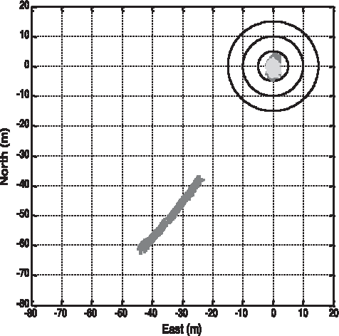
Scatter plot showing atypical errors for a GNSS receiver. The 60 m errors resulted because the orbital location of the satellite was changed without warning the user community through the navigation message.

Other human-made faults have occurred in the history of GPS. On occasion, the satellite hardware has introduced significant faults. For example, the so-called clock runoffs are the most common human-made faults. The GNSS satellites carry atomic clocks and these are typically very stable. On occasion, however, the clock time drifts away from GPS time quite rapidly, and the clock data contained in the navigation message do not keep up with this drift. On other occasions, the signal hardware (baseband or radio frequency) suffers a soft fault and the transmitted signal becomes distorted relative to the expected signal.^18,19

The human-made faults described above are potentially hazardous. In fact, the aviation community labels them as potential sources of HMI, because the errors can be large compared to the requirements for critical aviation operations such as airport approach and landing. Moreover, the probability of HMI is greater than the target level of safety for aviation. For these two reasons, the aviation community has developed a set of GNSS augmentations that detect these faults and warn the airborne fleet within seconds. These augmentations will be described in the Safety Augmentations that Monitor GNSS Performance section, but first we consider another important source of HMI: space weather.

Space Weather

The ionosphere surrounds Earth at altitudes from 70 to 1300 km, and introduces an additional delay in the travel time of the GNSS signal from orbit to Earth. Figure 11 is an example of the nominal ionospheric delay over the conterminous United States (CONUS). The data were collected on November 19, 2003, and the figure shows the delay as experienced if the satellite is directly overhead the receiver. As shown, these vertical delays vary from 3 to 7 m. For satellites closer to the horizon, the error can be three or four times greater than the delays shown in the figure. Even so, ionospheric delays are generally smooth over large areas. Figure 11 shows that the vertical delay varies only by a few meters over CONUS. Thus, ionospheric estimates made at a fixed reference receiver would be valid for hundreds of kilometers. More specifically, if we place GNSS receivers at airports, the ionospheric delays observed at the airport would be strongly correlated with the ionospheric delays experienced by an approaching aircraft.

Fig. 11.

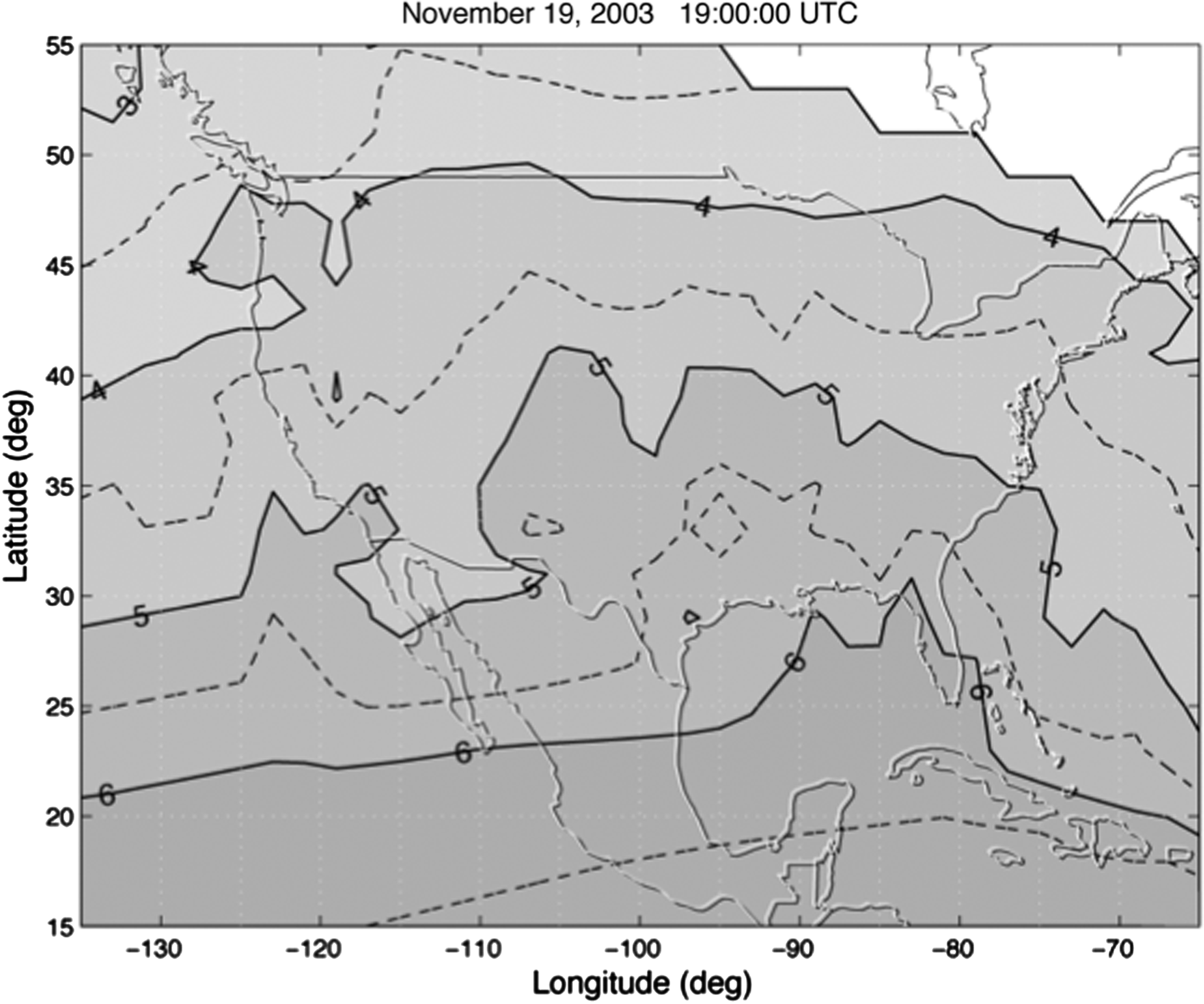
Vertical ionospheric delay over the conterminous United States on a day with calm space weather, November 19, 2003.

Figure 12 is an example of the ionospheric delay on the next day, November 20, which was a very disturbed day. As shown, the vertical delay now varies from 2 to 26 m. This variation is five times greater than that shown in Figure 11, and the spatial gradients are much sharper. The delay over Ohio changes by approximately 20 m over a 500 km distance. This corresponds to a gradient of around 40 parts per million (ppm). In fact, gradients as large as 400 ppm have been observed at the GNSS L1 frequency. Such sharp events need appreciable care especially when GNSS is used to support airport approach and landing operations.

Fig. 12.

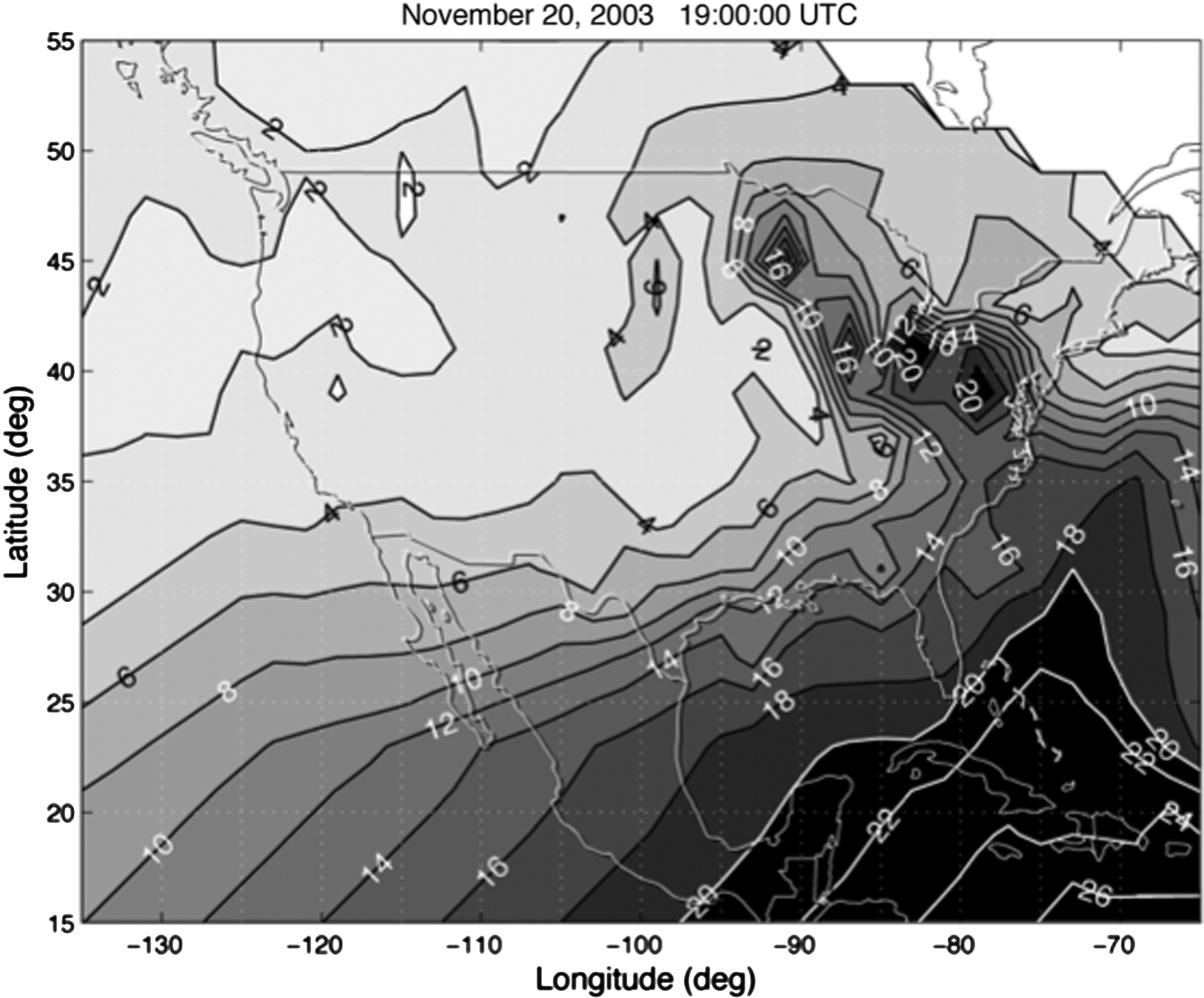
Vertical ionospheric delay over the conterminous United States on an ionospheric storm day, November 20, 2003.

Figures 11 and 12 show that solar activity can cause significant increases in the ionospheric delay and the associated spatial gradients. The delays might jump from nominal values of a few meters to tens of meters. The associated gradients may be 20 m or more over 500 km. Two of the augmentations described in the section Safety Augmentations That Monitor GNSS Performance are differential GNSS systems. They treat these errors by placing GNSS reference receivers at known locations. These ground measurements are broadcast to the airborne fleet and used to correct the airborne measurements. However, even this differential cure is not perfect, because strong space weather events can introduce the sharp gradients mentioned above. In these cases, the ionospheric delay measured at the reference station may not be strongly correlated with the delay experienced by the avionics. Large ionospheric storms can last for many hours and can occur over large portions of the United States. Hence, space weather effects on GNSS has been a major area of study for the last two decades.^20,21

Figure 13 shows the variation of space weather events with the 11-year solar cycle. More specifically, the figure shows the sunspot number. Sunspots are cool planet-sized events on the sun's surface that are associated with strong magnetic events on the sun. These solar events propagate through the solar system and can often cause ionospheric upsets here on Earth.

Fig. 13.

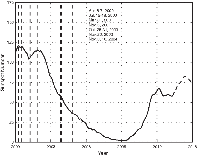
Sunspot numbers since the year 2000 show the last two peaks of the 11-year solar cycle. Ionospheric storms that caused outages of the vertical guidance normally offered by the Wide Area Augmentation System (WAAS) are also shown. The WAAS outages indicated by the dashed vertical lines have a duration of over 1 h.

A disturbed ionosphere can have another effect: scintillation. Scintillation is a rapid variation in the amplitude and phase of the received GNSS signals. These fluctuations can cause the GNSS signal power to drop by 10 dB or more. Such variations may only last for a few seconds, but they can break the continuity of the GNSS function in an aircraft. Scintillation is particularly prevalent in equatorial and polar regions, where an entire evening might suffer from sporadic scintillation. Thus, scintillation effects on satellite navigation is also a major area of current study.

Safety Augmentations That Monitor GNSS Performance

To cope with the challenges described above, civil aviation has augmented GPS to detect the human-made faults and space weather events. The probability of a human-made fault in the GPS system is approximately 10⁻⁵/h per satellite. The target level of safety for an aircraft navigation system is approximately 10⁻⁷/h, or one hundred times smaller than the observed failure rate. Similarly, space weather events, notably the ionosphere, can introduce location errors that may be potentially hazardous to the aircraft safety. These storms can occur several times per year during the peak of the solar cycle. In these peak years, the rate of these events is more than one hundred times greater than the target level of safety for aviation.

For these reasons, the civil aviation community has augmented GPS with systems that detect and remove errors due to these human-made faults and space weather. Three such augmentation strategies exist, and are now described. The ground-based augmentation system (GBAS) is described in the next section and provides integrity by comparing GNSS measurements to the known locations of three or four reference receivers located on the airport property. The space-based augmentation system (SBAS) compares GNSS measurements to the known locations of dozens of reference receivers spread over continental areas. RAIM does not use ground truth; it compares every GNSS range measurement to the consensus of the other satellites in view. All integrity techniques are based on a comparison, but GBAS and SBAS compare to ground truth, while RAIM compares to the other satellites in view of the aircraft.

Ground-based augmentation

As shown in Figure 14, GBAS are located at the airport to be served. Reference receivers monitor the GPS (or GNSS) signals. Since the reference receivers are at known locations, they can generate corrections to remove the nominal GPS errors. They also contribute to performance monitoring, generating alarms to flag satellites that cannot be reasonably corrected. GBAS also provides data that allow the aircraft to continuously estimate a protection level that should always be greater than the actual NSE. We say that the protection2 level overbounds the true error.

Fig. 14.

Ground-based augmentation system (GBAS). (Courtesy of BridgeNet International)

All the GBAS reference receivers are on the airport property. Thus, the corrections and alarms are valid within 100 km or so around the airport. They serve aircraft that are landing, approaching, or departing from the airport. GBAS is also capable of supporting aircraft that are maneuvering in the terminal airspace that surrounds the airport. Given this range of applicability, GBAS uses a line-of-sight radio to broadcast the performance monitoring information to the airborne fleet. This radio broadcast operates in the very high frequency (VHF) portion of the radio spectrum and is called a VHF data broadcast.

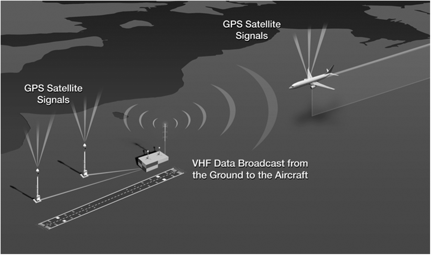
Space-based augmentation

SBAS spread their reference receivers across continental areas. As shown in Figure 15, some 38 stations are used to cover North America, and a similar number are used to serve the European airspace. As shown in the figure, these receivers send their GPS measurement data to master stations that generate corrections and error-bounding data that are valid over the area spanned by the reference network. Since the data are valid over continental areas, SBAS uses geostationary satellites to broadcast these navigation safety data to the airborne fleet. Figures 1 and 2 show these SBAS satellites.

Fig. 15.

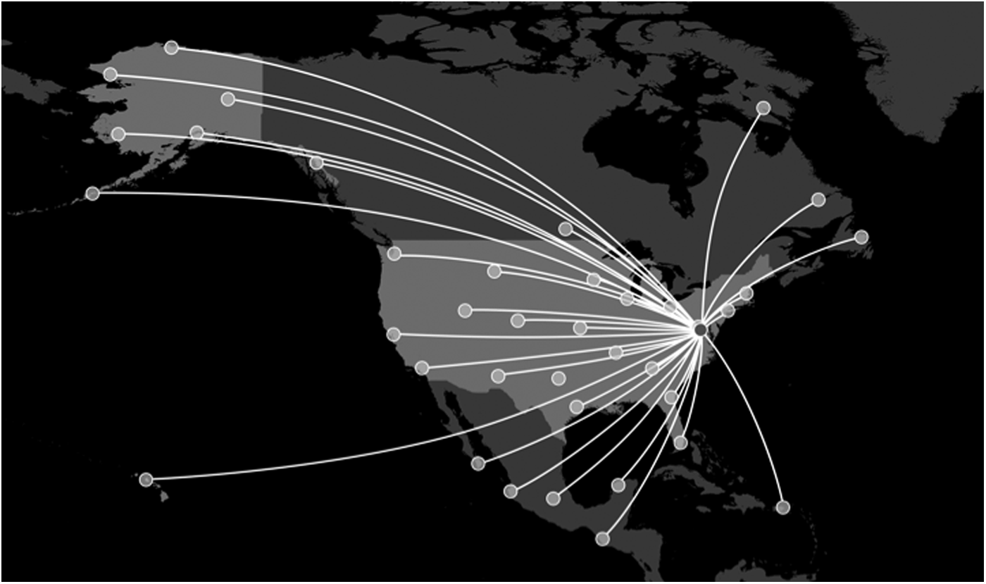
WAAS showing the connections between the reference receivers and the WAAS master station on the East Coast. (Courtesy of BridgeNet International)

The Wide Area Augmentation System (WAAS) is the SBAS for North America. Similar systems are operating in Europe and Japan, and are under development in India and Russia.

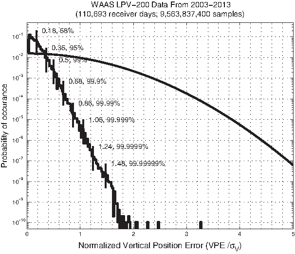
WAAS has been in operation since July 2003, and has served well. Figure 16 shows the cumulative distribution function (CDF) for WAAS vertical NSE. It shows 10 billion error measurements collected since the inception of WAAS in 2003. As shown, the largest error in this history is 14 m and it occurred once. We focus on two features of this NSE distribution. First, the core of the distribution covers the central 95% of the errors, and accuracy measures the width of this nominal core. As shown, WAAS vertical accuracy is 1.4 m. This is the typical day-to-day performance of WAAS.

Fig. 16.

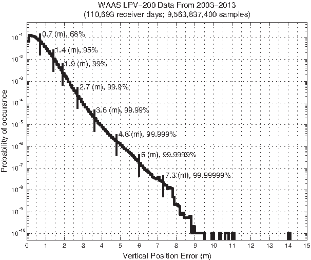
Cumulative distribution function (CDF) for vertical errors when using the WAAS. Accuracy measures the breadth of the core of the error distribution, and integrity manages the extent of the tails. (The data are from the FAA Technical Center.)

The tails of the CDF shown in Figure 16 are also important. These NSE tails are measured at 10⁻⁵, 10⁻⁷, or even 10⁻⁹. At these low probability levels, the tails include the potential impact of human-made faults (see section Faults in Systems or Procedures), space weather (see section Space Weather), and bad actors (see section Bad Actors: Jammers and Spoofers). As shown, WAAS has done a good job of managing these feared events, and thus the tails shown in Figure 16 are not heavy.

Navigation systems that detect NSE tail events with high probability are said to have integrity, and Figure 17 displays WAAS integrity. More specifically, it gives the CDF for the ratio between WAAS vertical errors and the WAAS-provided standard deviation for those vertical errors. This standard deviation is associated with the protection level mentioned earlier. Specifically, the NSE error distribution should be overbounded by a Gaussian distribution with zero mean and the WAAS-provided standard deviation. Figure 17 also gives 10 billion data points for the decade from 2003 to 2013. It shows that WAAS performance is much better than the Gaussian curve. A statistician would say that WAAS errors are leptokurtic, which means that the error are more concentrated toward zero than the Gaussian CDF with the same standard deviation. An aviator would simply be happy for a valid overbound of the true position error.

Fig. 17.

Histogram (or CDF) for the ratio of WAAS vertical errors to the WAAS-provided standard deviation for those vertical errors. (The data are from the FAA Technical Center).

Navigation systems that meet the RNP must have integrity and continuity. Continuity requires that the false alarm rate of the performance monitors be small. This requirement competes with integrity, because continuity breaks whenever an integrity alarm sounds falsely. Thus, the integrity monitors must be sensitive to real threats to navigation safety, but they must be specific to real threats; they should not false alarm and needlessly break continuity.

Receiver autonomous integrity monitoring

In contrast to SBAS and GBAS, RAIM is self-contained. In fact, RAIM belongs to a larger family of fault detection techniques that are known as aircraft-based augmentation systems. As mentioned earlier, SBAS and GBAS detect faults by comparing the GPS measurements to ground truth. RAIM compares the GNSS measurement from each individual satellite to the consensus of the other satellites in view. Mathematically, RAIM is based on the residuals of the individual GNSS measurements relative to the least-squares navigation solution based on all satellites in view.

RAIM is attractive because it does not need a ground reference network or a real-time broadcast from the ground network to the aircraft. However, RAIM fault detection is intrinsically weaker than the SBAS or GBAS capability, because it does not have access to ground truth. The navigation solution must be overspecified and the geometries of the underlying subset solutions must be strong. In principle, SBAS and GBAS can provide integrity even for an aircraft with only four satellites in view. In contrast, RAIM needs at least five satellites, because the navigation solution must be overdetermined. In addition, the five subsets created by deleting one satellite at a time must all have a strong geometry, so that the subfixes will have reasonably good accuracy. This means that RAIM fault detection frequently requires six or even seven satellites in view.

For this reason, RAIM has not yet been used for vertical guidance. However, it has been approved for lateral guidance, and approximately 200,000 aircraft carry RAIM worldwide to enable lateral guidance in the enroute, terminal area, and nonprecision approach phases of flight.

As mentioned earlier, GNSS will eventually be based on a multiplicity of full constellations: GPS, GLONASS, Galileo, and BeiDou. With the advent of these new constellations, RAIM may be able to support vertical navigation. After all, the geometric diversity from two or more constellations will mean that all navigation solutions will be overspecified and that the subset geometries will be stronger. The air navigation community is researching this possibility, and has developed a concept known as advanced RAIM or ARAIM. ²²

To provide vertical guidance, ARAIM includes a set of requirements on the core GNSS constellations. These requirements must be met and verified periodically if the core constellation is to be included in the suite of measurements used by the avionics to support vertical navigation. If ARAIM can be proven to be safe, then it may be able to support navigation down to altitudes of only 200 feet over the airport surface. Since ARAIM would be a multiconstellation capability, it would be independent of the health of any one of the core GNSS constellations.

Bad Actors: Jammers and Spoofers

All of the GNSS satellites are placed in MEO, and the signals must travel 20,000–24,000 km before they reach the surface of Earth. Thus, these signals are extremely weak when they reach the Earth's surface; their received power is approximately 10⁻¹⁶ W. In principal, navigation satellites could be placed closer to Earth to strengthen the received power, but these closer constellations would need many more satellites to guarantee that four (or more) satellites are in view of every user.

Radio signals with terrestrial origin can easily overwhelm the weak GNSS signals. If malevolent signals are sent to deny the GNSS service, then they are called jammers. If these signals are counterfeits of the GNSS signal, they are called spoofers. The latter is more pernicious than the former, because spoofers are designed to introduce a hazardous position error without detection. Taken together, jammers and spoofers are the bad actors of GNSS.

In recent years, the GNSS community has been particularly dismayed by the prevalence of personal jammers. These devices intentionally emit a signal in the GNSS portion of the frequency spectrum. They are designed to jam GNSS tracking devices placed surreptitiously on automobiles to secretly track the location of the driver. These personal jammers certainly serve their purpose, but they also jam all GNSS use in the immediate neighborhood of the automobile under surveillance. Personal jammers were particularly problematic at Newark International Airport. A GBAS prototype was placed at this airport with its antennas and reference receivers all within a few hundred meters of the New Jersey Turnpike. Unfortunately, vehicles traveling on that highway carry personal jammers and would occasionally jam the GPS receivers at Newark; the GBAS test system was collateral damage.

Today, the overall operational impact of GNSS jamming on aviation is limited by the continued presence of the navigation aids that preceded GNSS. These systems include VHF omnidirectional range (VOR), distance measuring equipment (DME), and the instrument landing system (ILS). These are all terrestrial radio systems and they are still in operation. ²³ VOR and DME support navigation for aircraft operating in domestic enroute and terminal airspace and for nonprecision approaches at airports. ILS is used to guide aircraft as they approach and land at airports. Together, these systems support all current conventional navigation operations. However, as aircraft operations transition to performance-based navigation, the conventional systems cannot provide a suitable backup to GNSS for the operations described in the section Efficiency and Environmental Benefits.

For this reason, the aviation community is developing alternative position navigation and time (APNT), which is essentially a reconfiguration of existing FAA ground-based transmitters to provide RNAV and RNP. If successful, APNT would become a key element of the next generation air transportation system (NextGen).

One variant of APNT is called hybrid APNT, which would combine signals from DME and the radio transmitters (RTs) that are being deployed to support dependent surveillance by air traffic control.^24,25 Both of these signal sources are ground based and of high power; thus, they are difficult to jam. In addition, these signals will be plentiful in the United States, which already has approximately 1,100 DME stations and plans to have approximately 700 RTs. DME and RT both radiate in the ARNS band that extends from 960 to 1215 MHz. Figure 18 shows this radio band, which is also shown on the left-hand side of Figure 4.

Fig. 18.

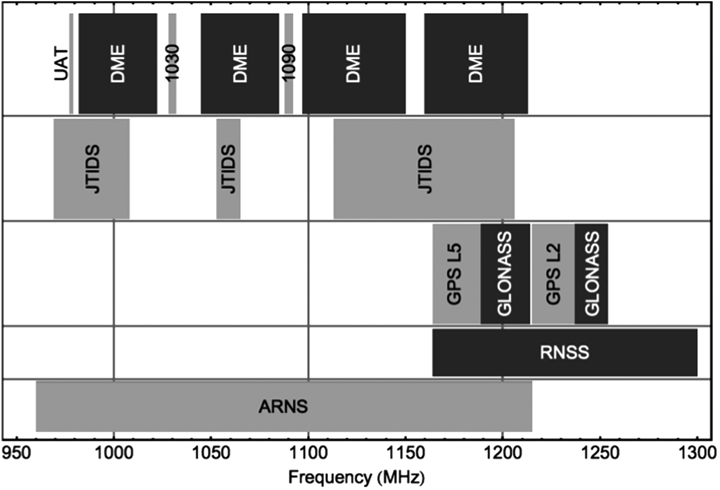
Aeronautical radio navigation system (ARNS) radio spectrum that includes hybrid APNT. This band is from 960 to 1215 MHz, and is also shown on the left-hand side of Figure 4. The spectral blocks labeled DME contain many channels for signals from distance measuring equipment (DME). The blocks labeled 978, 1030, and 1090 are used for air surveillance, and the blocks labeled L2 and L5 are GNSS frequencies. The blocks labeled JTIDS are used by the military for the Joint Tactical Information Distribution System.

Hybrid APNT would also combine two kinds of ranging: one-way and two-way. One-way ranging is a synonym for pseudo-ranging used by GNSS and described at the beginning of this section. In the case of APNT, the one-way ranging signals would be sent from the ground to the aircraft, and the aircraft would passively receive these one-way signals; the aircraft would not respond. Hybrid APNT uses baro-altimetry for estimating altitude, and so one-way ranging would require three APNT signals from the ground to estimate the aircraft's longitude, latitude, and clock offset.

To reduce the required signal count from three to two, hybrid APNT would also use two-way ranging. Indeed, today's DME is based on two-way ranging. The aircraft initiates by sending a signal and the ground station responds when it receives the aircraft signal. The aircraft measures the round-trip travel time, subtracts the ground station turn-around delay, and divides by two. Thus processed, the measurement estimates the one-way travel time. Unlike pseudo-ranging, this two-way technique is not passive; the aircraft must radiate. Thus, capacity is a concern when many aircraft are initiating ranging transactions. However, APNT would use two-way measurements sparingly. It would track the one-way range of all APNT transmitter in view, and generate two-way measurements from a single DME in view. In this way, hybrid APNT would be able to estimate the clock offset for the avionics, and require only two stations in view to estimate longitude and latitude. Thus, hybrid APNT would not threaten DME capacity.

Finally, hybrid APNT would integrate inertial sensor products as they become available. The inertial sensors will extend APNT coverage downward to small and medium-sized airports that are not equipped with landing systems. Thus, most airports will have a backup approach aid should GNSS be jammed. Such an operation is depicted in Figure 19.

Fig. 19.

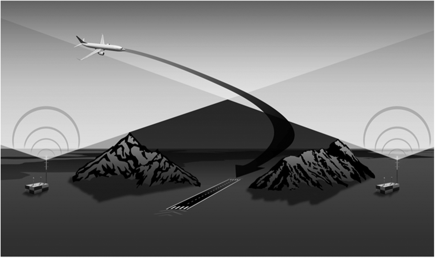
Role of inertial sensors in alternate position navigation and time (APNT). As the aircraft descends, terrestrial signals are obstructed and APNT would use inertial sensors to sustain lateral navigation as the aircraft descends from strong radio coverage into weak radio coverage. (Courtesy of BridgeNet International)

In addition to APNT, the aviation community is developing a suite of techniques to combat jamming and spoofing. For example, new GNSS satellites broadcast on two aviation frequencies (e.g., L1 and L5 for GPS). In other words, the new GNSS signals offer frequency diversity, and the aviation community is developing dual-frequency avionics to make use of L1 and L5. With a second frequency, airborne users of GNSS would be much less vulnerable to accidental RFI, because they would have a backup frequency. In addition, the L5 signal is intrinsically more resistant to RFI, because it uses a broader spectrum, and so it provides some protection against intentional attacks. ²

In addition, the community is developing techniques to detect spoofing. Some of these are based on receiver autonomous tests and others could be network based. For example, the GNSS receiver could periodically compare the GNSS and APNT position fixes to fend off spoofers.

Summary

Hopefully, this introductory article has described the air operations that will use satellite navigation to save fuel and reduce the environmental impact of aviation. These operations are based on the RNAV and RNP capabilities of GNSS. These capabilities enable unrestricted point-to-point flight paths; flight is no longer restricted to the pathways dictated by ground-based radio navigation. They enable aircraft to fly direct from departure to destination using the most fuel-efficient routes and to avoid complicated terrain at low altitude. They provide the flexibility to design new procedures that enable aircraft to fly closer together to increase the arrival and departure rates and fly continuous climb and descent operations to minimize fuel consumption, noise, and carbon emissions.

Satellite navigation supports complicated approaches and departures that cannot be served by the straight beams that emanate from ground transmitters. It also supports OPDs, where the aircraft floats down to the ground in accord with its own aerodynamics. These maneuvers save fuel and reduce ground noise. In time, GNSS will support terminal area operations that feather arriving aircraft into the arrival pattern rather than requiring all new aircraft to go to the end of the arrival queue. Finally, GNSS will also support enroute aircraft that wish to take advantage of changes in the wind, even then these changes occur after departure.

This article has also strived to teach the basics of safety for air navigation based on GNSS. Indeed, GNSS is augmented to meet the performance monitoring demands of RNP. The GNSS augmentations detect the known feared events that would threaten safe navigation. They broadcast protection levels to the airborne fleet, and this information is used to overbound the true position errors in real time. The feared events include faults in the GNSS systems and procedures, space weather, and bad actors (spoofers and jammers).