
Abstract
Abstract
Mass spectrometry is an analytical technique for the characterization of biological samples and is increasingly used in omics studies because of its targeted, nontargeted, and high throughput abilities. However, due to the large datasets generated, it requires informatics approaches such as machine learning techniques to analyze and interpret relevant data. Machine learning can be applied to MS-derived proteomics data in two ways. First, directly to mass spectral peaks and second, to proteins identified by sequence database searching, although relative protein quantification is required for the latter. Machine learning has been applied to mass spectrometry data from different biological disciplines, particularly for various cancers. The aims of such investigations have been to identify biomarkers and to aid in diagnosis, prognosis, and treatment of specific diseases. This review describes how machine learning has been applied to proteomics tandem mass spectrometry data. This includes how it can be used to identify proteins suitable for use as biomarkers of disease and for classification of samples into disease or treatment groups, which may be applicable for diagnostics. It also includes the challenges faced by such investigations, such as prediction of proteins present, protein quantification, planning for the use of machine learning, and small sample sizes.
Introduction
Machine learning techniques have been utilized broadly to analyze data from many areas of biology; in particular, various machine learning methods have been applied to data generated by the analytical techniques of transcriptomics and metabolomics for classification of unknown samples and identification of genes relevant to the disease state. Similar methods are now being applied to the field of proteomics and, more specifically, the analysis of data generated from tandem mass spectrometry (Sun and Markey, 2011).
There are numerous technologies used to extract quantitative protein information from biological samples. These techniques cover a broad spectrum of approaches, balancing throughput (one/many proteins at a time) and quality of the extracted data.
Commonly used techniques include two-dimensional gel electrophoresis, enzyme-linked immunosorbent assays (ELISAs), protein arrays, affinity separation, and mass spectrometry-based technologies (Ray et al., 2011; Schiess et al., 2009).
A number of these methods, including gels and ELISAs, are limited in the number of proteins they can analyze because of time requirements. They also require specific proteins of interest to be chosen when designing the study and suitable cross-reactive antibodies to be available; this can be challenging for non-model organisms. In comparison, mass spectrometry (MS) techniques can be used as a high-through-put discovery based method; lists of proteins can be identified from samples that are analyzed (Perkins et al., 1999). This means that tandem mass spectrometry can be used to find proteins that may not have previously been considered, provided the proteins can be found within protein sequence databases. A combination of multiple proteomics methods can also be utilized to form an effective analysis pipeline. Ray et al. (2011) showed that MS, in various guises, has been pivotal to biomarker discovery for a range of different diseases. This review will discuss the applications of machine learning for analysis of proteomic mass spectrometry data and the challenges involved. MS-specific challenges, including the identification of proteins using sequence database searching software and protein quantitation or pre-processing for peak analysis, will be covered. As will machine learning-specific considerations, such as the small numbers of samples that can often result from an MS investigation, and the types of machine learning most suited for the required task, either sample classification or biomarker identification. A survey of articles involving the combination of mass spectrometry and machine learning will be followed by a brief discussion of post-machine learning analysis, including literature mining and pathway analysis. An overview of the areas to be covered in this review is provided in Figure 1.
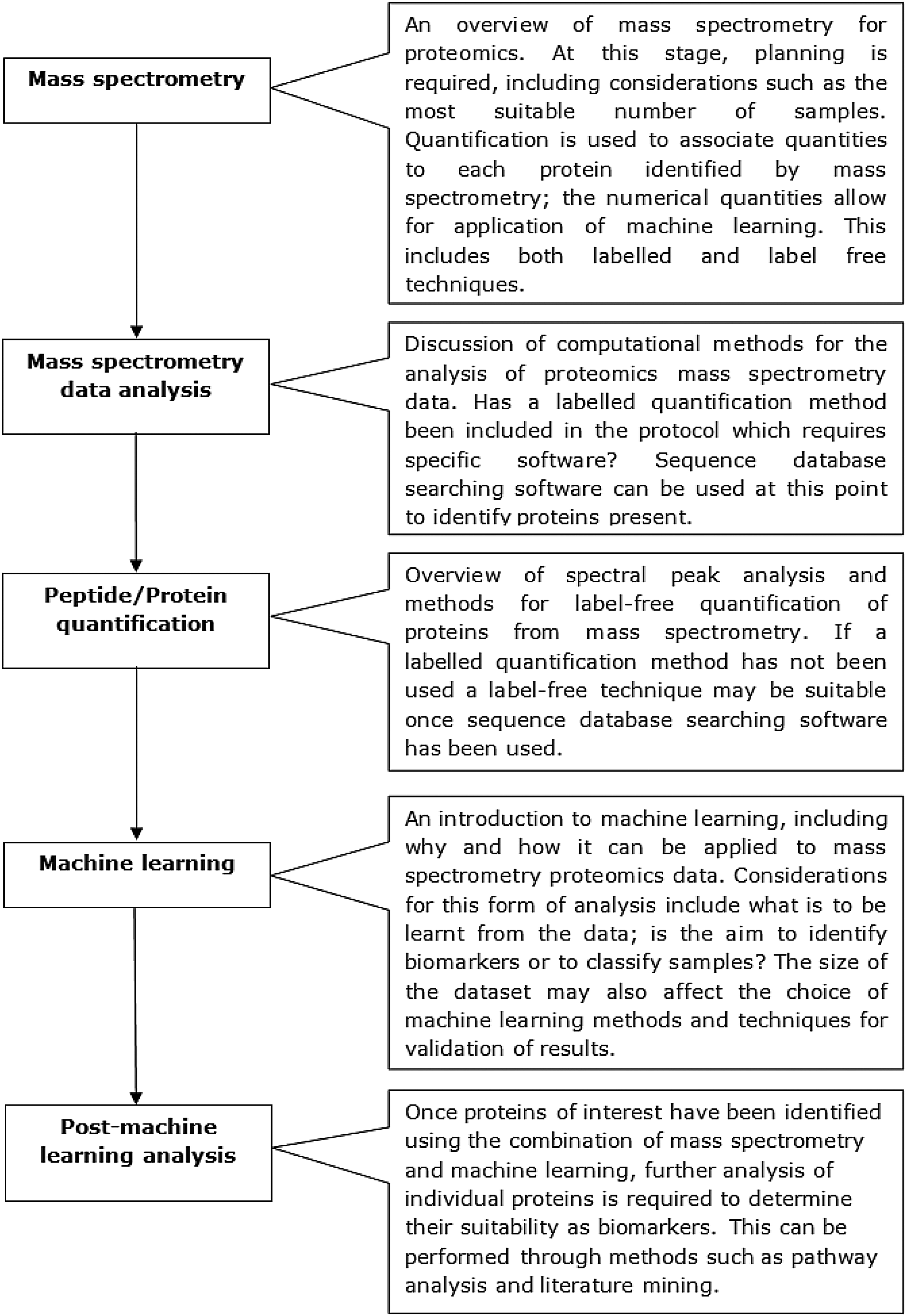
An overview of the topics covered in this review, including the general work flow required and the major considerations that are necessary before beginning an investigation combining mass spectrometry and machine learning.
Proteomic Mass Spectrometry Workflow
Overview
MS is used to measure the mass-to-charge ratio (m/z) of molecules, however, prior to MS taking place, the molecules must first be electrically charged and changed to gas phase; this is due to the electromagnetic fields involved in the mass analyzer stage of MS (Walther and Mann, 2010). Electrospray ionization (ESI) (Fenn et al., 1989) is a common method used for the ionization of molecules, however other methods are becoming increasingly popular, including matrix-assisted laser desorption/ionization (MALDI), from which surface-enhanced laser desorption ionization (SELDI) has been developed (Domon and Aebersold, 2006; Yates et al., 2009). ESI has been further developed to form nano-ESI, a technique that offers a number of benefits including smaller analyte requirements, greater tolerance of contaminants, and higher sensitivity to hydrophilic compounds (Schmidt et al., 2003; Wilm and Mann, 1994). After molecules have been transformed to gas phase, their m/z ratios are measured by their movement through an electric or magnetic field, this occurs in a mass analyzer. There are a number of different types of mass analyzer, including quadrupole, time-of-flight (TOF), ion trap, and Fourier Transform (FT). These systems each have different strengths and weaknesses, such as the range of m/z values that can be detected and the mass spectrometric resolution. Some mass analyzers can also be used in combination, such as Quadrupole-TOF, for identifying more complex molecules. Once measured, the m/z values are visualized as mass spectra, which describe the molecules present through peaks at the relevant m/z values (Aebersold and Mann, 2003).
In proteomics, the most widely used method for protein identification using MS is known as the “bottom-up” approach. Using this approach, the molecules measured are peptides, which are generated by the enzymatic digestion of the peptides in a sample (McLafferty et al., 2007). This approach determines the m/z values for the peptides present, collision-induced dissociation (CID) is then applied during which peptides are fragmented by collision with an inert gas, such as helium (Walther and Mann, 2010). The final stage of MS includes a detector, which is used to record and amplify the amount of ions at the different m/z values. The m/z values are then visualized using mass spectra. The resulting spectra from the fragmented peptides, known as tandem MS spectra (MS/MS), are generated wherein the peaks describe the amino acids present in the peptides (Aebersold and Mann, 2003). Yet, this only provides the identifications of the peptides that are present in the sample after enzymatic digestion occurred and so it is still necessary to work back from the known peptides to predict which proteins were originally present in the sample. This process can be accomplished, from the MS/MS data, by sequence database searching software, such as Mascot (Cottrell, 2011), this is discussed further in a later section. The “bottom up” approach is in contrast to the “top-down” method, for which MS is used to directly analyze undigested proteins, through the ionization and dissociation of the intact proteins in the mass spectrometer. This approach can be more specific than “bottom-up,” however, it has greater experimental requirements and requires more complex instruments (McLafferty et al., 2007) for it to be applicable to a global scale analysis.
Opportunities and challenges of mass spectrometry data analysis
The use of mass spectrometry for the discovery of proteins has opened up a number of opportunities; however, there are also technical and conceptual challenges that need to be overcome and these will vary from study to study.
A major role for the identification of proteins using mass spectrometry is the discovery of biomarkers of disease (Diamandis, 2004). Biomarkers can be used for a variety of different purposes. They can be used to determine if a biological process is taking place. They can also serve as indicators for the diagnosis or prognosis of disease and to determine the course of progression of a known disease. Biomarkers can also be used to investigate the efficacy of treatments and interventions or existing or investigational drugs (Williams, 2009).
Another opportunity that mass spectrometry provides is viewing proteins on a network level or in functional pathways. Understanding the expression of proteins in a pathway can provide essential knowledge in the changes involved during progression of disease as well as identification of potential drug targets (Ashburner et al., 2000; Bassel et al., 2011; Kanehisa and Goto, 2000; Neilson et al., 2011).
MS is not always suitable due to some limitations; it is often impractical to produce large numbers of samples due to time and financial constraints. Furthermore, a high-through-put approach is not always required (Aebersold and Mann, 2003). There is also some difficulty in finding proteins of interest if they are at low abundance, when compared to other proteins within the sample, which is often the case for proteins that may be suitable as disease biomarkers (Horgan and Kenny, 2011; Ray et al., 2011). Another challenge in mass spectrometry proteomics is unambiguously identifying the proteins from the peptides identified, mainly due to a lack of sequence data for some species (Tan et al., 2009). Another challenge is the quantification of proteins (Neilson et al., 2011). Methods include both labeled, such as stable isotope tagged peptides, and computational label-free techniques. Label quantification techniques are not always appropriate for certain experimental systems, in which case label-free methods can be applied (Neilson et al., 2011). Protein quantitation is discussed further in a later section.
Mass Spectrometry Data Analysis
Overview
Tandem MS generates large data files containing lists of many peaks that are used to identify peptides. The implementation of computational methods is necessary for processing, to identify proteins that relate to the identified peaks and to compare samples. In most cases, mass spectrometry data analysis follows one of the paths that are summarized in Figure 2. The first, shown on the left of Figure 2, looks directly at MS peaks and their intensities (Katajamaa and Oresic, 2005). The second uses sequence database search engines to identify which proteins are present (Perkins et al., 1999). The second method is also used in conjunction with protein quantification techniques (Neilson et al., 2011), which can be applied during preparation of samples before mass spectrometry, or during the data analysis phase, in the case of label-free methods.
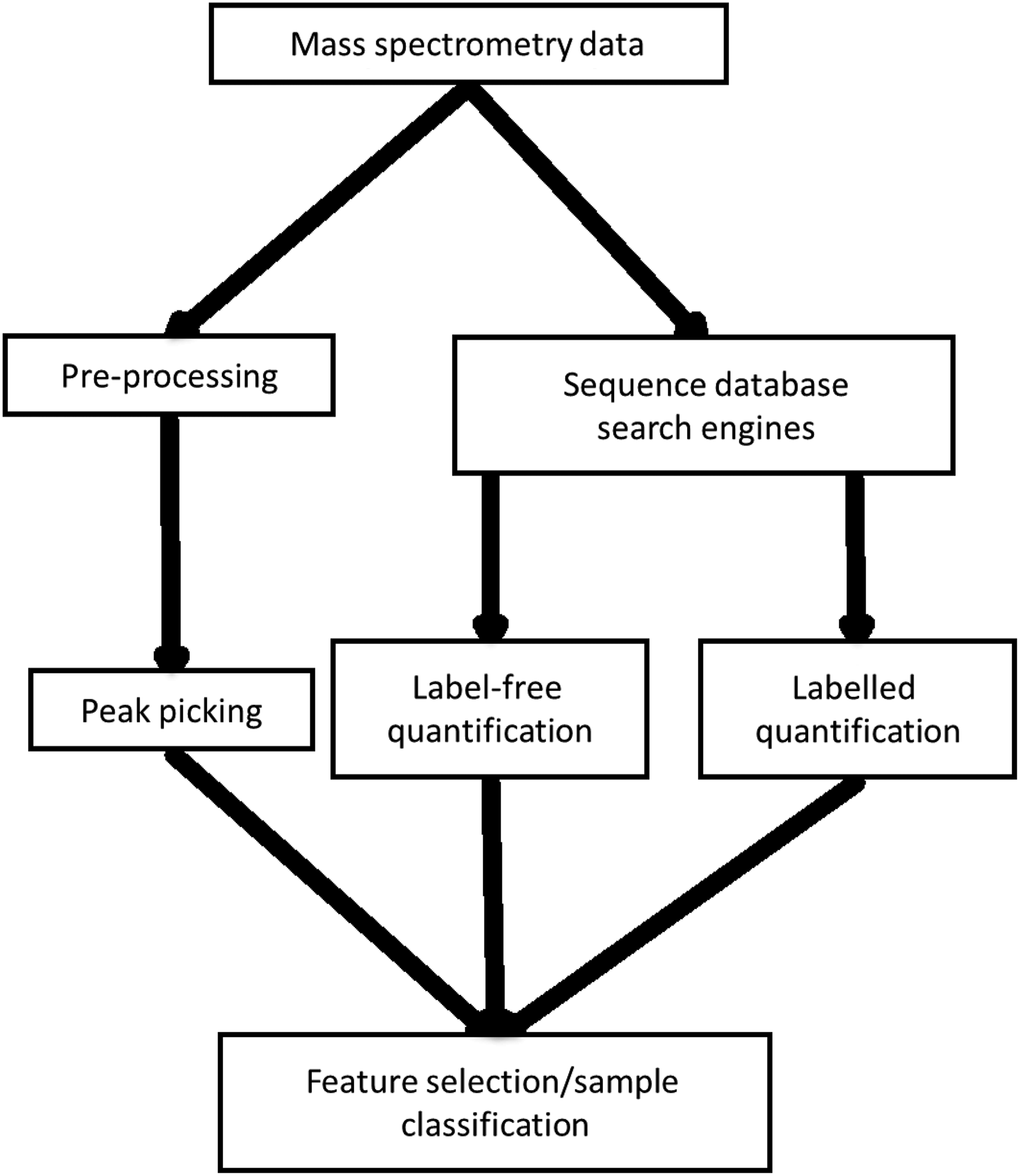
Proteomics mass spectrometry data analysis workflow. The workflow diverges into two sections; the first involves peak picking and application of machine learning directly on mass spectral peaks. This is in comparison to the second section, which involves quantification of proteins, either labeled or label-free, followed by machine learning.
Various software packages are used at different stages of the workflow shown in Figure 2. Some frequently used tools are detailed in Table 1.
Peak picking
In peak picking, the mass spectra produced are analyzed without actually determining which peptides or proteins are present, instead peaks with significantly high signal intensities are considered as possible biomarkers. There are some drawbacks to this method. First, this is not a direct method for finding proteins present in a sample, and further analysis is required. Second, thorough pre-processing of the peak data is essential, including normalization, peak alignment, and noise reduction (Katajamaa and Oresic, 2005). Without these pre-processing steps it is not possible to compare the same peaks in different samples accurately, and errors generated at this stage will be transmitted through to further analyses (Roy et al., 2011).
Search engines
During tandem mass spectrometry, peptide masses are identified that are present in the samples analyzed. These peptide masses in conjunction with the masses of their fragments are then used to determine which peptides are present and the proteins to which they relate. Sequence database searching software, such as Mascot (Perkins et al., 1999), have been developed to discover which proteins are most likely to be present. These software work in conjunction with protein sequence databases, such as UniprotKB (Jain et al., 2009) and NCBInr (http://www.ncbi.nlm.nih.gov/), as well as species-specific databases, including sgn for Tomato (http://solgenomics.net/) and Tair for Arabidopsis (http://www.arabidopsis.org/); they assess the peptides present and, by comparison with the equivalent masses/fragment masses calculated from known protein sequences found in the associated databases, protein identities are predicted. This method is not completely accurate because of the similarity of some protein sequences and the small proportion of the overall protein sequence to which the identified peptides may relate (Neilson et al., 2011; Perkins et al., 1999). Also, protein identifications can only be made if they are present in the interrogated database. However, various metrics are reported alongside proteins to show the probability that the correct identification has been made (Cottrell, 2011).
Protein quantification
There are two main types of mass spectrometry-based protein quantitation: labeled and nonlabeled. The former involves added steps during the sample preparation, prior to mass spectrometry, but can be performed in a variety of ways (Bantscheff et al., 2012; Neilson et al., 2011). Chemical and peptide labeling approaches are common, a frequently used example of this is iTRAQ (Boehm et al., 2007). Other label quantification methods include those that label proteins metabolically, for example, stable isotope labeling by amino acids in cell culture (SILAC) (Ong et al., 2002). Another method, Selected Reaction Monitoring (SRM), which is used for targeted quantitation, involves the selection of ions during the second mass spectrometer phase of MS/MS (Gillette and Carr, 2013; Lange et al., 2008). Finally, there are methods that result in absolute protein quantitation, including those that use stable isotope labeling standards, such as AQUA and QconCAT (Beynon et al., 2005; Gerber et al., 2003). There are some reasons why labeled quantitation methods are not always appropriate or possible, including expensive isotope labeling, a limit on the number of samples that can be analyzed, and an incompatibility with some sample types. They must be included in the design of the experiment and so are only suitable if quantitation has been planned from the outset. To quantify proteins without these additions to the methodology, label-free quantification techniques are available (Neilson et al., 2011).
There are two types of label-free quantification methods: measurement of signal intensity and spectral counting. The first method uses area under the curve of spectral peaks (AUC) to compare amounts of peptides present in samples. The second method sums up all MS/MS spectra seen for peptides from a single protein (Neilson et al., 2011). There are many label-free quantitation software available, including both commercial and open source. Examples of freely available AUC methods include MSInspect (Bellew et al., 2006) and MSQuant (Schulze and Mann, 2004). A basic method of spectral counting, emPAI, is automatically included by Mascot when identifying proteins. Other examples of spectral counting software available for quantification of proteins include PepC (Heinecke et al., 2010) and APEX, which can be used for label-free quantitation (Lu et al., 2007; Vogel and Marcotte, 2008).
Whilst computational label-free methods can be simpler to implement because of their reduced laboratory requirements, the samples being analyzed only come together in silico (Neilson et al., 2011). This allows for more variation to occur during sample preparation, which can be partially avoided using labeled methods because samples, once labeled, are brought together at as early a stage in the workflow as possible.
Quantitative methods provide numerical values related to the proteins that are discovered by mass spectrometry; this is advantageous when machine learning techniques are to be applied to identify biomarkers or classify samples. Whilst there are other experimental proteomic techniques that can be used to quantify proteins, such as Western blotting (Voshol et al., 2009; Wilm, 2009), which are discussed in a later section, these methods are not comparable with the level of throughput that can be achieved using mass spectrometry (Bantscheff et al., 2007).
Machine Learning
Machine learning involves generating programs that improve their performance when undertaking a certain task, based on its experience. Machine learning can take various forms, which can be applied when each sample has been annotated with a quantitative label (Mitchell, 1997; Yang, 2010); here we will be focusing on the application of supervised machine learning to mass spectrometry data. Supervised machine learning involves training a model based on data samples that have known class labels associated with them. This is in contrast with unsupervised classification, or clustering, where no samples have associated class labels, and instead samples with similar attribute profiles are grouped together.
This section introduces the concept of supervised classification and six types of machine learners: Bayesian classifiers, Rule-based learners, Decision trees, Random Forest, Support Vector Machines, and Artificial Neural Networks. These methods are also summarized and compared in Table 2. This is followed by a brief discussion of feature selection, which involved the selection of significant attributes for reduction of datasets, with the aim to increase the accuracy of classification models which are then applied to the features selected. Finally, this section discusses the evaluation of classification models, to determine how well they classify datasets. This includes simply dividing the data into training and test sets or using a form of cross-validation. Text box 1 describes some terms associated with sample classification.
The speed of learning and ease of interpretation rows rank the methods 1 to 6, with 1 being the best (Kotsiantis, 2007).
Classification methods
Supervised machine learning can be used for classification; a model is built from training data, which includes class labels for each sample, by assessing values of the attributes. The model is then used to determine the class of each sample in a dataset, which has no such labels, known as the test set (Kotsiantis, 2007; Larrañaga et al., 2006). Classes can be different phenotypes, such as disease groups or treatments. Attributes can be the peak mass-to-charge ratio values or identified proteins. Classification can be used, for example, in diagnosing diseases, as the model should determine between healthy and diseased samples. It is also possible to consider the specific attributes as biomarkers for the defined classes (Abeel et al., 2010; Saeys et al., 2008).
Bayesian classifiers
Bayesian classifiers are statistical methods based on Bayes theorem (Casella and Berger, 2002). Naive Bayes (John and Langley, 1995) is the simplest of this group; it works by estimating the probability that each sample input belongs to each of the classes. It is said to be ‘naïve’ because it assumes that attributes are independent of each other. Despite this assumption, Naïve Bayes has shown to be a very competent machine learning method across many application domains and has excellent scalability.
Rule-based learners
This group of learners includES BioHEL (Bacardit et al., 2009) and JRip (Cohen, 1995). Their purpose is to automatically generate sets of human-readable rules (e.g., ‘IF Attribute A >2 AND Attribute B <4, THEN Class=One’) that explain why a certain group of samples belongs to a class (e.g., treatment group) of a problem (Fürnkranz, 1999). Rule learning is a very broad family of methods. Their differences depend (a) on the type of rule sets they generate (e.g., ordered/disordered rule sets, crisp/fuzzy rules) and (b) on how to build the rules (e.g., using a constructivist heuristic/using a global search method such as a genetic algorithm), and the rule sets (e.g., generating at once all the rules in a rule set/constructing a rule set iteratively).
Decision trees
Decision trees are machine learning models that structure the knowledge used to discriminate between examples in a tree-like structure. Figure 3 shows a simple decision tree, which divides a dataset into its three classes based on the values of two attributes. Simple decision trees are very easy to read to understand how the classification has been built and which attributes it uses. New instances are classified by following the tree along the relevant branches, depending on the attributes of the sample. Methods, such as C4.5, start with an empty tree and iteratively split the data, creating branches of the tree, until they decide to assign all examples of a branch to a specific class, creating a leaf of the tree, based on a certain criteria (e.g., all examples in the node belong to the same class/the error in the branch of the tree is small enough (Quinlan, 1993).
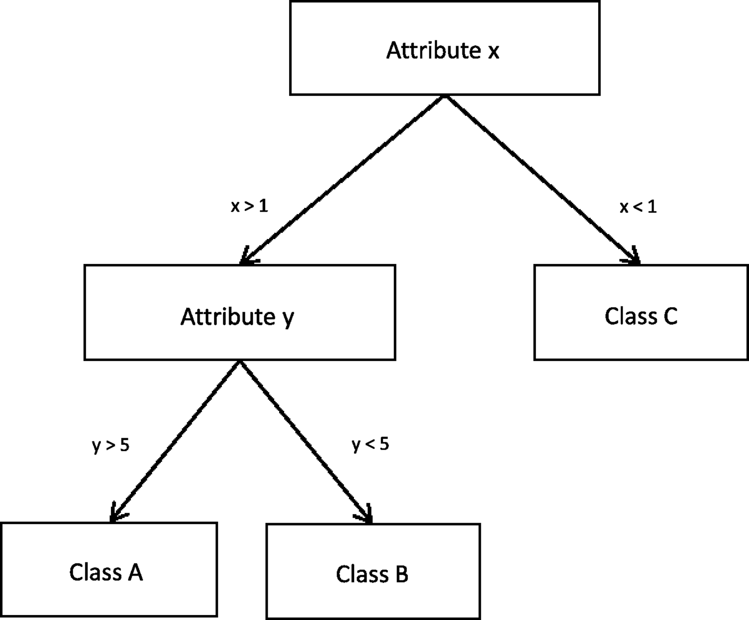
A simplified Decision Tree that divides data into its three classes, based on two attributes.
Random Forest
The Random Forest method builds on that of decision trees, wherein multiple trees are built from the training data. Each tree has only access to a randomly sampled subset of the attributes of the problem. Then, when predicting the class of the test samples, each individual tree predicts a class and the majority class predicted among the trees is used (Breiman, 2001).
Support Vector Machines
Support Vector Machines (SVMs), shown in Figure 4, are a class of machine learning that base their prediction in the concept of linear separability between classes. The characteristics that specifically define SVMs are (a) the criteria they use to define the optimal linear classifier based on the concept of separation margin maximization, (b) the identification of the so-called support vectors, the minimal set of training instances that are necessary to define the optimal linear classifier; because they lay at the edges of the margin, and (c) the use of kernels to transform the original set of variables into a higher order non-linear space in which the linear separability happens. The Sequential Minimal Optimization (SMO) is one of the most popular SVM algorithms (Platt, 1999).
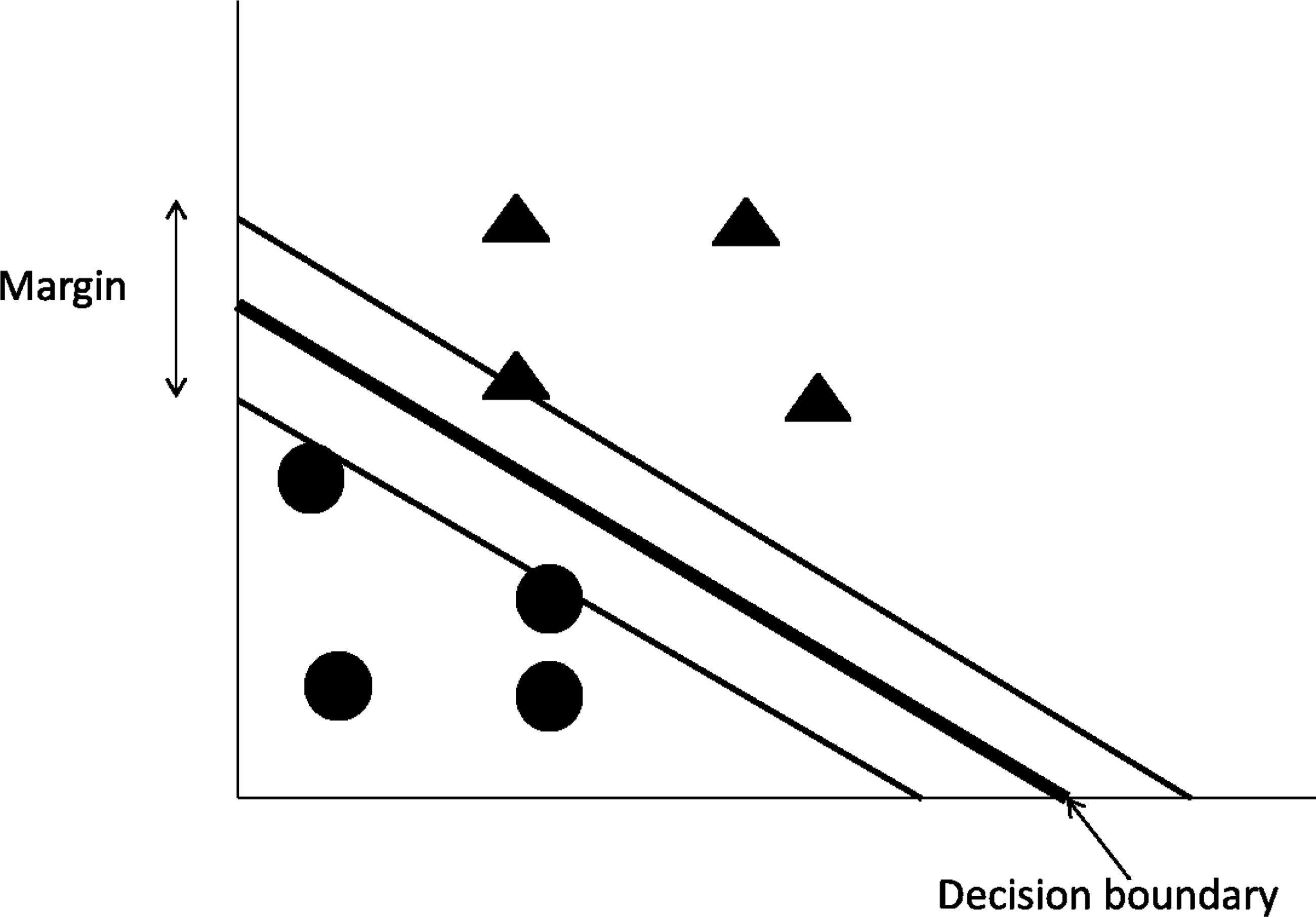
A graphical representation of Support Vector Machines and the linear division of two classes.
Artificial Neural Networks
Artificial Neural Networks (ANNs) are inspired by the workings of the brain. ANNs are composed of a collection of computational elements (neurons) that are connected between them using a very broad variety of interconnectivity patterns. The connections of a neuron determine whether it becomes activated, based on the signal they receive. Generally each neuron is a variant of a linear classifiers, but the inclusion of multiple neurons and layers result in the construction of sophisticated nonlinear classifiers that allow for their application to complex problems (Dayhoff and DeLeo, 2001; Mitchell, 1997). A representation of ANNs is shown in Figure 5.
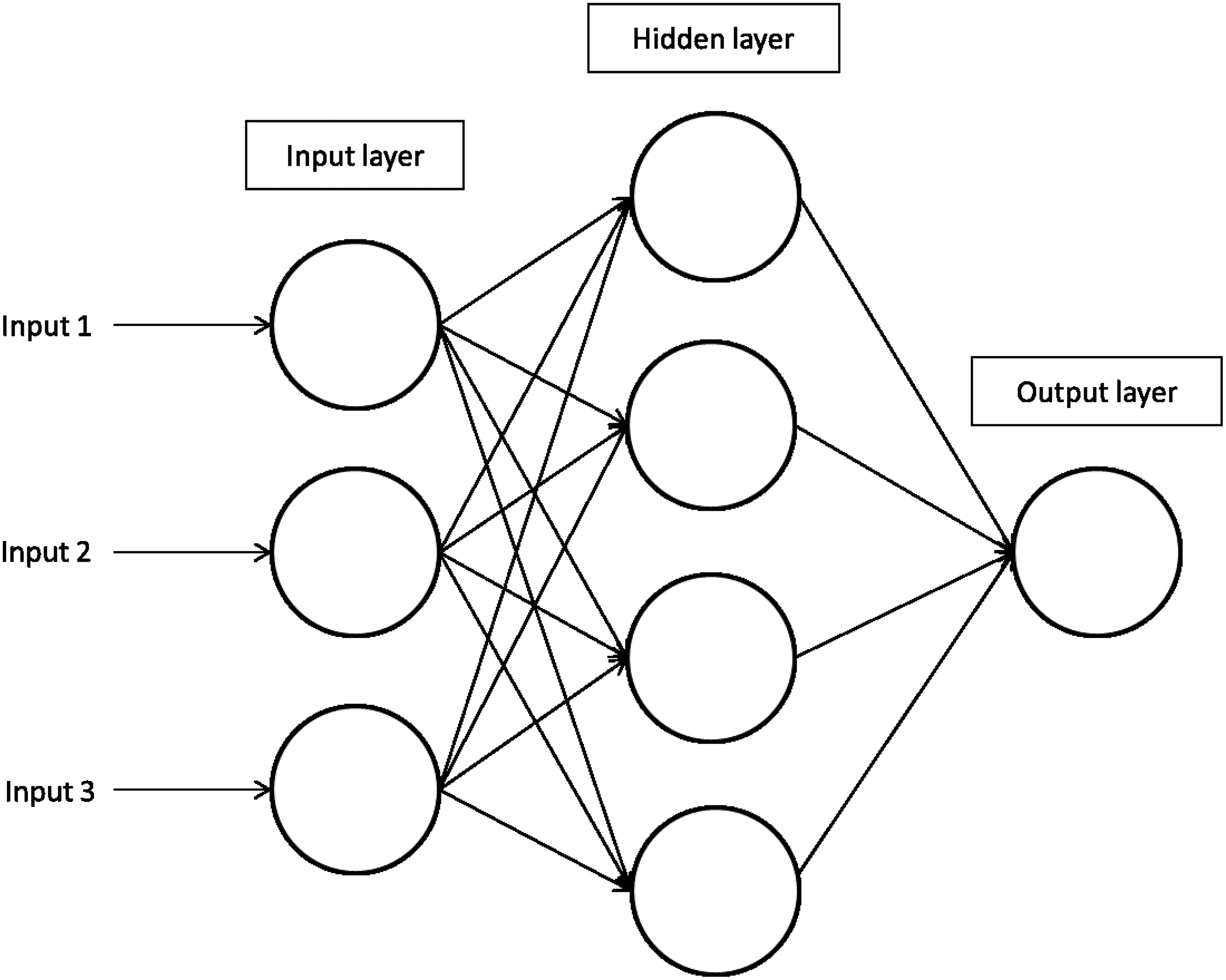
A representation of Artificial Neural Networks and the layers involved in the generation of a model.
Feature selection methods
Feature selection methods have the primary role of selecting significant attributes, through removal of redundant or irrelevant attributes, and therefore can also be used for biomarker identification. These methods are applied to proteomics MS data to identify proteins, which vary significantly between treatments or disease groups, either individually or in combination with others, and therefore could be potential biomarkers (Abeel et al., 2010).
Feature selection methods can be used prior to classification techniques, as pre-processing, to reduce the size of a dataset by selecting a subset of attributes, on which a learner is then applied (Saeys et al., 2008). This can involve removing redundant, irrelevant, or noisy data (John et al., 1994; Kohavi and John, 1997). Feature selection can be used to reduce the number of attributes because redundant data have been shown to reduce the accuracy of classifiers. Some classifiers, such as decision trees, are affected more by irrelevant data, compared to, for example, Bayesian classifiers (John, 1997).
Many feature selection methods are based on machine learning techniques that have already been discussed, such as Naïve Bayes (Duda, 2001) and support vector machines (Guyon and Elisseeff, 2003; Weston et al., 2003).
Validation procedures for machine learning methods
Evaluation of classification models is essential to determine their ability and accuracy; ideally this would be performed by producing the model on a training set and testing it on an independent test set. This is not always possible when the number of samples is limited, which is often the case when working with proteomics data, because of limitations in time and cost of producing many repeats of samples. When an independent testing dataset is not possible, cross-validation can be used, as it splits up a single dataset into training and test sets. Using 10-fold cross validation, the dataset is split up ten times, producing ten training sets each consisting of 90% of the data and ten test sets containing the remaining 10%. There are also other variations of cross-validation; another commonly used method is leave-one-out cross-validation where only one sample is used for the test set and there are training and test set combinations equivalent in number to the number of samples available (Ambroise and McLachlan, 2002; Kohavi, 1995).
Whilst cross-validation is useful for analyzing small datasets it does have disadvantages, the main one being over-fitting. As a result models may appear to perform better when tested using cross-validation than when tested on an independent dataset, although some classification algorithms are less prone to over-fitting than others. Therefore larger datasets would be more suitable, because cross-validation would not be needed to generate training and test sets (Kohavi, 1995; Varma and Simon, 2006).
Machine learning has been used to classify samples across a variety of diseases (Larrañaga et al., 2006). Table 3 summarizes eleven investigations that reported the use of machine learning techniques for the classification of samples, after analysis with MS. This includes application to both peak data and quantified proteins. The articles were identified by querying both PubMed (http://www.ncbi.nlm.nih.gov/pubmed) and Google Scholar (http://scholar.google.com/) for the search terms ‘machine learning’ and ‘proteomic mass spectrometry’, optionally followed by the term ‘biomarkers’. The search was done first without the term ‘biomarkers’ so that articles applying machine learning to proteomics data which did not include the identification of biomarkers could also be retrieved (searched January 2013).
Investigations have been grouped based on related disease.
Classification accuracies are reported with the percentage of samples correctly assigned to their relevant classes; this can be generated either using a test dataset or cross-validation. From the investigations surveyed, cross-validation was a popular method for generating training and test sets, as it particularly useful when there is a limit on the number of samples it is possible to produce. There were a range of cross-validation techniques used; the most popular was leave-one-out cross-validation, but others, including 10-fold and 3-fold were used. The alternative is to split the dataset up into training and test sets. This was performed for the datasets with larger numbers of samples. One investigation compared both cross-validation and splitting up the dataset and found the best classification accuracy, for their dataset, using leave-one-out cross-validation (Guan et al., 2009). However, this result is specific to this dataset and so it would be useful to perform similar analyses on other datasets, as not all datasets would give the same results. As a result of the majority of studies using cross-validation, many reported a further requirement would be to repeat their analysis on larger datasets. Table 3 includes information on the percentage accuracy, and the machine learning method used. It is also necessary to consider how the data are split up into separate classes. Bloeman et al. (2011) included both diagnosed and nondiagnosed asthma samples in their dataset. With these samples considered in one class, as classification accuracy of 100% was achieved, however when they were split into two different classes, the accuracy of the model lowered to 73%.
Table 3 shows that a variety of machine learning methods were used for the classification of samples, with SVMs the most popular choice, being used in four of the eleven investigations surveyed. These analyses included the use of both proprietary and open source software, many applying machine learning to actual peak data, rather than quantified proteins. One article (Guan et al., 2009) provides a good example of increasing classification accuracy by combining a classifier with a feature selection method. Alone, the best SVM classifier evaluated on that dataset achieved an accuracy of 83.3% when assessed with leave-one-out cross validation, however this was increased to 97.2% when combined with an SVM-based feature selection method. However, it is impossible to compare accuracies achieved across different datasets because the datasets result in problems of varying difficulties. It can be useful to compare accuracies of different methods used for the same dataset, for example where different parameters for SVMs were tested, as well as the comparison of various feature selection techniques, to identify which combination of feature selection and classifier work best together (Willingale et al., 2006).
Biomarker discovery
Machine learning can also be useful in determining which proteins, from MS data, could be used as biomarkers to differentiate between samples of different classes (Saeys et al., 2008). Table 3 also includes information from investigations on the application of machine learning on mass spectrometry data for the identification of the most suitable biomarkers, based on factors such as the ability to test for proteins in a clinical setting; this includes both identified proteins and mass spectral peaks as biomarkers. Further analysis, following identification of peptides or proteins as putative biomarkers, are then required, as it may be that the proteins identified would not actually be suitable for use as biomarkers. For example, body fluids such as urine and serum (blood) are regarded as being most suitable fluids to search for biomarkers because they are easier to obtain for assessment purposes during diagnostic tests and treatments. Also, blood is pumped around the body by the circulatory system and bathes cells, tissues, and organs, thus carrying putative protein biomarkers around the body before being processed by the liver and filtered by the kidneys into urine (Pang et al., 2002; Veenstra, 2007).
Table 3 shows that the number of possible biomarkers identified varies greatly between studies, due to differing complexities of data, for example, Ratcliffe et al. (2009) identified only two m/z values as biomarkers, and Ralhan et al. (2008) formed a panel of three biomarkers. This is in comparison to Guan et al. (2009) and Oh et al. (2009) who identified 38 and 26 putative biomarkers, respectively. Some found biomarkers that had previously been identified; this is both useful as support for the previous investigations, and as some validation to the methods being newly applied to the area. Other investigations identified biomarkers that work specifically well together and so formed panels of markers. In Fan and Chen (2009), different panels of biomarkers were compared and those markers that worked best together were identified. The development of panels of biomarkers is useful as using multiple biomarkers may reduce false positives as it removes dependence on individual proteins, and allows proteins that are detected for different diseases to be useful (Williams, 2009).
To discriminate between samples, the majority of the studies applied machine learning to only the peaks from the mass spectrometry data that correspond to peptides. To facilitate the development of diagnostic assays and/or inform the underlying biology at a molecular level, peptide biomarkers require further investigation.
Literature mining and pathway analysis
Machine learning has been shown to highlight important peptides/MS peaks, however further analysis is required to determine to which proteins they relate. In the case of machine learning applied to quantified proteins, literature mining is also useful for understanding the biological relevance of the proteins identified as potential biomarkers. It may be important to discover more information about interacting proteins and pathways in which they have a role (Hur et al., 2009; Jenssen et al., 2001; Tsuruoka et al., 2008); by doing this, it can be determined whether the identified proteins may become useful biomarkers and which processes would be measured. Pathway analysis can be used to narrow down, or provide a focus to, the search for biomarkers by determining which pathways they participate in (Lawlor et al., 2009).
Literature mining is also essential in discovering more information after machine learning has been applied to MS peaks, however identification of the proteins the peaks relate to is first required (Oh et al., 2009).
Tools such as Ingenuity Pathway Analysis (http://www.ingenuity.com) and DAVID (Huang et al., 2008, 2009) can be used to facilitate literature mining and pathway analysis, or information can be mined directly using such article databases as PubMed (http://www.ncbi.nlm.nih.gov/pubmed).
Machine Learning and Other –Omics Technologies
There are many other techniques generating large datasets from biological samples, for which machine learning approaches are beneficial. These methods, including transcriptomics, metabolomics, and lipidomics, can also be used in conjunction with proteomics to gain a broader view of the biological system under analysis (Joyce and Palsson, 2006; Silvestri et al., 2011; Tan et al., 2009).
Other proteomics methods include Western blots, dot-blots, ELISAs, protein arrays, and antibody arrays. However, these techniques cannot achieve the same high-throughput as MS/MS and therefore the data generated would not be suitable for machine learning and do not require this level of analysis (Bantscheff et al., 2007; Voshol et al., 2009; Wilm, 2009).
Transcriptomics has historically been dominated by microarray technologies, but now next generation sequencing is becoming more popular, due to its greater sensitivity, larger dynamic range, and advantage of not being limited by detecting only genes that are present on arrays (Mardis, 2008). Both microarrays and next generation sequencing have the high throughput capabilities that MS/MS does, and therefore are suitable for machine learning (Tan et al., 2009). Yet there can be large differences in mRNA and the actual abundances of proteins (Lawlor et al., 2009).
The main techniques used for the study of the metabolome are MS, preceded by either gas or liquid chromatography and NMR (Joyce and Palsson, 2006; Tan et al., 2009). Commonly, large libraries of peaks are used to identify metabolites, such as lipids, amino acids, and sugars, to match the peaks identified by MS. Metabolomics can also be considered as a method complementary to proteomics. It may be that the metabolites are amplified in comparison to the related proteins, and therefore more likely to be identified by MS/MS (Tan et al., 2009).
Future Research Directions and Priorities
Machine learning has been successfully applied to proteomics data, yet it can still be used for other purposes and across a wider range of diseases. For example, the investigations discussed in Table 3 show machine learning has been used largely on the proteomics of cancers; therefore there are many other diseases and biological systems which would benefit from the application of machine learning.
Rule-based learners, as well as being used for classification, are suitable for the identification of biomarkers, as the attributes that are used frequently in rules are those that are better at discriminating between classes. Rule-based machine learning has also been applied to microarray data to develop gene interaction networks based on genes that are used together in rules (Bassel et al., 2011; Glaab et al., 2012). This method could be applied to mass spectrometry data in the same way, generating networks from groups of proteins that appear together in rules.
There are also other methods that were originally developed for transcriptomic data, such as gene set analysis (Luo et al., 2009), that could be modified for application to proteomics. Furthermore, machine learning could be combined with literature data to include background knowledge, which is not necessary for machine learning to be applied, but could improve the data analysis process (McKinney et al., 2006).
Summary
This review discussed the use of machine learning applied specifically to proteomics data for classification of samples and identification of biomarkers, although machine learning can be applied to other omics data. Investigations that involve multiple types of omics data can also aid in the identification of biomarkers, for example, investigations into potential biomarkers in cartilage and chondrocytes are using both transcriptomics and proteomics data (Lewis et al., 2013; Mobasheri, 2012; Williams et al., 2011). Machine learning analysis requires large datasets and so it is essential to consider the number and type of samples that will be generated and their suitability for the application of machine learning.
The applications of machine learning discussed here have demonstrated that there are many different methods suitable for both classification of samples and identification of novel biomarkers. Therefore, to undertake such an investigation requires the consideration of a number of matters, summarized in Table 4. Various methods should be tested to identify which is most suitable for the dataset. There is also a necessity for further biological evaluation of any protein that is identified from mass spectrometry as a suitable biomarker. This can be performed using both laboratory-based and computational methods, as biomarkers not only need to be differentially expressed, but other factors, such as ease of sourcing the sample, must be taken into account.
Further analysis of proteins identified as possible biomarkers is essential. Pathway analysis is used to verify relationships between proteins found by machine learning. Pathway analysis can also be used to understand where proteins that have been identified as possible biomarkers act, for example, if one protein is upregulated during progression of a disease, does it result in other proteins being up- or downregulated.
It can also be seen from the investigations surveyed that the majority of diseases analyzed are cancers and therefore there are many other areas for these methods to be applied.
Finally, machine learning can be applied to mass spectrometry data to generate networks that indicate protein interactions. This is a method that has previously been applied to microarray data, and is also now applicable to proteomics.
Footnotes
Acknowledgments
This work received financial support from the Biotechnology and Biological Sciences Research Council (BBSRC) (Contract Grant number: BB/F017014/1), the WALTHAM Centre for Pet Nutrition, and the European Union Seventh Framework Programme (FP7/2007-2013) under grant agreement no. 305815. The BBSRC had no involvement in the study design, data collection, analysis, and interpretation. The decision to submit the article for publication was not influenced by the funding body. The authors would like to thank Bruker UK for their collaborative support.
Authors' Contributions: All authors have made substantial intellectual contributions to the conception and design of the study, data acquisition, analysis, and interpretation.
Author Disclosure Statement
The authors declare that they have no competing interests or financial disclosures. AM is the coordinator of the D-BOARD Consortium funded by European Commission Framework 7 program (EU FP7; HEALTH.2012.2.4.5–2, project number 305815, Novel Diagnostics and Biomarkers for Early Identification of Chronic Inflammatory Joint Diseases). JB and SL are also members of the D-BOARD Consortium.