Gene Expression Data Analysis Using Closed Itemset Mining for Labeled Data

Abstract

Abstract

This article presents an approach to microarray data analysis using discretised expression values in combination with a methodology of closed itemset mining for class labeled data (RelSets). A statistical 2 × 2 factorial design analysis was run in parallel. The approach was validated on two independent sets of two-color microarray experiments using potato plants. Our results demonstrate that the two different analytical procedures, applied on the same data, are adequate for solving two different biological questions being asked. Statistical analysis is appropriate if an overview of the consequences of treatments and their interaction terms on the studied system is needed. If, on the other hand, a list of genes whose expression (upregulation or downregulation) differentiates between classes of data is required, the use of the RelSets algorithm is preferred. The used algorithms are freely available upon request to the authors.

Introduction

Microarray technology enables simultaneous examination of expression levels of thousands of genes in a single experiment. From a biologist's perspective, this is a substantial improvement over the more traditional experimental approach where typically only a single gene was examined. From a data analyst's point of view, microarray technology offers a great challenge simply because of the nature of the data. Instead of having large numbers of sample observations for a few variables, microarray data usually comprise thousands of gene variables but only a few samples (Lee, 2004). This is why several novel data analysis approaches have been implemented to address this task. Generally, microarray data analysis can be divided into two tasks: grouping of genes to discover patterns of biological behaviour, and the identification of specific genes of interest (Wu, 2001).

Depending on the goal of the study, statistics or data mining techniques are applied. When the goal is grouping of genes with similar biological function, both statistics and data mining address two types of tasks: supervised and unsupervised learning. For unsupervised learning, with the goal of finding patterns in gene expression, clustering methods are usually used. Classical clustering methods, such as hierarchical clustering, k-means clustering, self-organizing maps (Tamayo et al., 1999) have all been used for microarray data analysis. Methods for assessment of clustering results, for example bootstraping, have also emerged (Kerr and Churchill, 2001). When the goal of the experiment is to find genes with expression levels that differ significantly between classes of samples, or to find genes that accurately predict the class of the sample, supervised learning methods, such as decision trees and discriminant analysis, can be used (Butte, 2002).

When wishing to identify genes that are differently expressed between two classes under study, microarray data can be analyzed with the proper statistical models. Linear models are often used, but mixed-effects models are also becoming increasingly popular as an analytical tool (Wernisch et al., 2003). The difference between them is that mixed models incorporate random sources of variation (e.g., different people hybridizing different arrays within the same experiment). Regardless of the statistical model or learning method used, there is a risk of overfitting the model to the experimental data. That is why model complexity should be kept as low as possible; and the real challenge is to determine the optimal degree of model complexity that a given data set can support (Allison et al., 2006).

In the data mining/machine learning community, microarray data analysis can be approached through subgroup discovery with the goal of finding a set of rules for the target class.

The RelSets algorithm (Garriga et al., 2008) applied in this study employs relevancy filtering (Lavrač et al., 1999) in data preprocessing, followed by rule construction through closed itemset mining (Carpineto and Romano, 2004) to discover all relevant rules within a minimum true positive count constraint. For a better understanding of the paper, certain terms are introduced in Table 1.

Table 1.

Glossary of Data Mining and Statistical Terms Used in the Article

Term	Definition
Feature	Logical variable representing attribute-value pairs, for example, attribute → gene x; value → upregulated; feature → gene x is upregulated.
Closed itemsets	In data mining result, usually a large number of frequent patterns are extracted. Closed itemset mining is an approach to extract pattern describing rules from the dataset. Closed sets for labeled data represent relevant combinations of features that discriminate between the classes (e.g., sensitive and resistant potato cultivars).
RelSets	Algorithm for finding closed sets for class-labeled data (in our case resistant and sensitive potato cultivars). The result of RelSets is a set of nonredundant rules for describing the class: IF Closed set THEN Positive class.
Example	In the experiments presented, an example consisted of two microarrays of one trasgenic line or cultivar from two different post infection times (see gray ellipse in Fig. 1).
Minimum support constraint	When it is undesired that rules cover less than a certain number of positive examples, a reasonable minimum support constraint (MSC) is applied. An MSC of 1 defines that rule R must cover at least one training example.
Relevancy filtering	It has the purpose of eliminating features that are irrelevant for the ruleconstruction (Lavrač and Gamberger, 2006). In our case an irrelevant rule would be, for example, that an upregulation of gene X determines both class sensitive AND class resistant. This gene is irrelevant and thus filtered out in data preprocessing.
tp	True positive; number of positive examples that correctly cover a rule.
fp	False positive; number of positive examples that incorrectly cover a rule.
M value	log2 fold change of gene expression levels between the compared genes, usually expressed as \documentclass{aastex}\usepackage{amsbsy}\usepackage{amsfonts}\usepackage{amssymb}\usepackage{bm}\usepackage{mathrsfs}\usepackage{pifont}\usepackage{stmaryrd}\usepackage{textcomp}\usepackage{portland, xspace}\usepackage{amsmath, amsxtra}\pagestyle{empty}\DeclareMathSizes{10}{9}{7}{6}\begin{document}\begin{align*}\log_2 \frac{\rm x}{\rm y}\end{align*}\end{document} . An M value of 2 represents a four times increase in expression of gene x compared to gene y.

The input to RelSets is a dataset with class labeled examples and one parameter: the minimum true positive count (min TP). This is a constraint that implies that only rules that cover at least TP positive examples should be constructed. The RelSets algorithm works as follows. First, closed itemsets are mined in the positive class with a minimum support constraint (min TP). These closed sets can be directly interpreted as rules: \documentclass{aastex}\usepackage{amsbsy}\usepackage{amsfonts}\usepackage{amssymb}\usepackage{bm}\usepackage{mathrsfs}\usepackage{pifont}\usepackage{stmaryrd}\usepackage{textcomp}\usepackage{portland, xspace}\usepackage{amsmath, amsxtra}\pagestyle{empty}\DeclareMathSizes{10}{9}{7}{6} \begin{document} \begin{align*} {IF \ Closed \ set \ THEN \ Positive \ Class} \end{align*} \end{document}

These rules have high true positives count because they were built with a min TP constraint. It has been proven (Garriga et al., 2008) that these are all the most specific rules that have the potential to be relevant. In the second phase RelSets confronts the rules found in the first phase with the negative data. It removes relatively irrelevant rules on the negative data. In this phase a maximum false positives count constraint could also be applied.

The RelSets algorithm is complete in the sense that it finds all the most specific rules satisfying the minimum true positive count constraint. The algorithm is also nonredundant because in finds only the relevant rules. This makes the algorithm very appropriate for microarray data analysis because a small number of examples are available and the complete search of the space is very adequate. Also, as the results are to be interpreted by experts, redundancy is undesired as it would lead to more complex results hindering rule interpretability.

In this article we present a novel approach to microarray data analysis using discretised expression values in combination with the methodology of closed itemset mining for class labeled data (RelSets). The relevance of this analytical approach is evaluated through its comparison with statistical 2 × 2 factorial design analysis. Validation of the approach is done using the permuted microarray dataset.

A scientific question in this study is the effect of a specific kind of treatment on the target organism. In our study the target organisms are potato plants, infected with potato virus PVY, which is one of the agronomically most important potato pathogens. Sometimes the question in mind is finding genes that were differentially expressed after the treatment, thus giving the possibility of better insight into target organism response. We tried to find solutions to the task of finding specific genes of interest: (1) genes that are significantly differentially expressed after a given time of infection, and (2) genes that determine a class of plants resistant or sensitive to the viral infection.

Materials and Methods

Experimental design and preprocessing

Two experimental data sets were used in the experimental setup. In the first, four transgenic potato lines (two of them resistant and two of them sensitive to a viral infection) were tested. Plants from each transgenic line were divided in four subsamples: one half was infected with potato virus Y ^NTN (PVY^NTN) and the other one was mock inoculated. Mock inoculation served as control for mechanical damage. Plants were harvested at two time points, 8 and 12 h after infection. In the second experimental dataset, two potato cultivars (one sensitive and one resistant to infection with PVY^NTN) were tested. The division of plants into subsamples was analogous to that above, and two time points after infection (30 min and 12 h) were used.

Every experiment was performed with at least three biological replicates, thus yielding 24 microarrays for the first experiment and 13 microarrays for the second. Each microarray was hybridized with a subsample inoculated with virus and a mock infected subsample from the same resistance type. Figure 1 illustrates the two experiments.

FIG. 1.

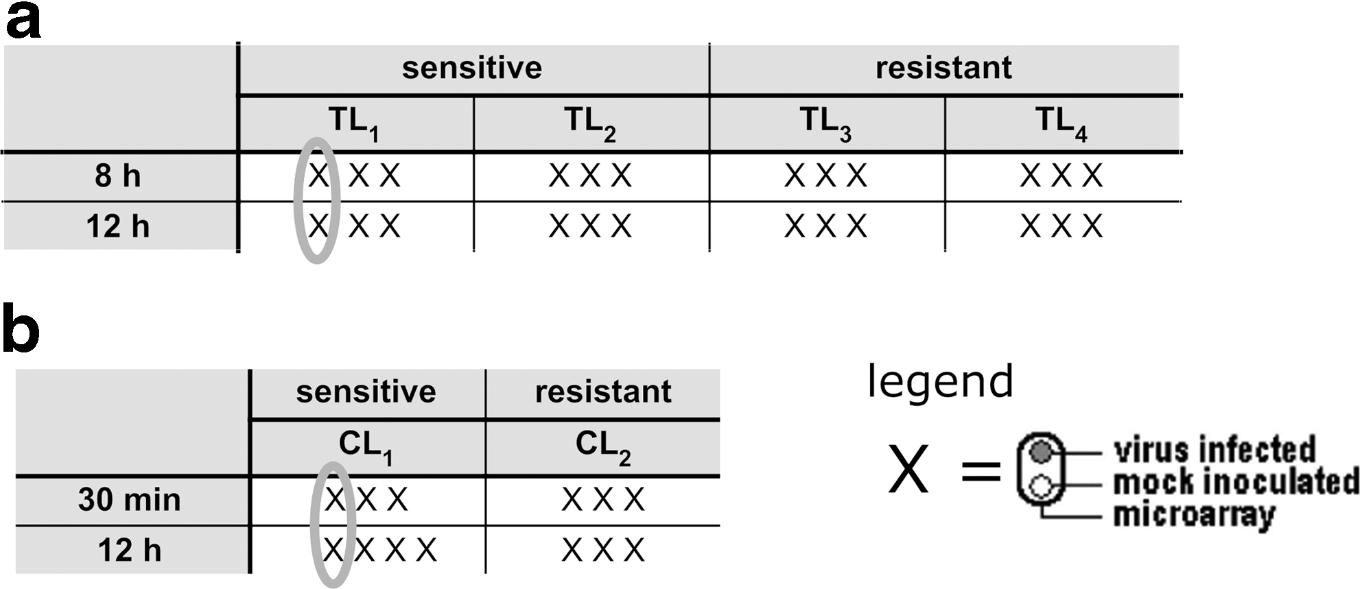
Schematic representation of the (a) first experimental dataset (b) second experimental dataset. The “X” in the table represents one microarray (thus, one biological replicate), consisting of a mock infected sample and a virus infected sample (see the legend). The number of “X” denotes the number of replicates for a particular sensitivity/time experimental combination. The gray ellipse around two microarrays from two different time points represents one example. TL, transgenic line, four in total; CL, cultivar, two in total.

Potato 10k cDNA microarrays (http://www.jcvi.org/potato/sol_ma_microarrays.shtml) were used, in which, excluding controls, 15,600 clones are spotted in duplicate. The initial data dimensions were therefore 31,200 × 24 for the first experiment and 31,200 × 13 for the second (also see Fig. 1). Quality control was performed using the image analysis software ArrayPro Analyzer^®. Spots that were unevenly shaped and had a low signal-to-noise ratio and low intensity signal on both channels (red and green), were not included in further analysis. Background correction half, implemented in one of the Bioconductor packages, limma (Smyth, 2005) was performed where background was subtracted from foreground intensities. Data was normalized using the loess and vsn normalization (Cleveland, 1979). Within-array spots were averaged and, for statistical analysis, the information about intraspot correlation was also taken into account (Smyth et al., 2005). Three weight values for one averaged array spot were possible: (1) weight = 0 where both spots within one array were flagged out; (2) weight = 1 where one of the spots was flagged out, and (3) weight = 2 where both spots passed the initial quality control. Data analysis of the two experiments was done separately.

Data discretization and application of RelSets Algorithm for microarray data analysis

We first define the term example (see Table 1). The first dataset is composed of 12 examples and the second of 6 examples.

First, filtering was done (see Table 2). The genes that had weight = 0 were marked as missing (NA). Next, if, for at least one of the possible factorial levels, that is, experimental conditions [e.g., sensitive (sen) Time 1 or resistant (res) Time 2] there were NA values for the replicates, then the gene was filtered out. After filtering, data dimensions were reduced to 10,397 × 24 for the first experiment and to 11,464 × 13 for the second experiment. Feature relevancy (e.g., if the same pattern of P or A values was obtained in sensitive and resistant examples, see also Table 1) was checked. There were no irrelevant rules in the first experiment and three genes were irrelevant and removed in the second one.

Table 2.

Filtering of Selected Genes as a Step in Data Preprocessing

Gene name	Sen Time 1	Res Time 1	Sen Time 2	Res Time 2	Outcome
STMHJ51	1.3 0.3 NA	NA NA − 0.5	0.1 NA − 0.1 − 1.1	NA NA NA	filtered out
STMIG44	NA NA NA	NA NA NA	0.5 − 0.3 NA NA	−1.0 − 1.4 NA	filtered out
STMCV26	NA NA NA	NA NA − 0.4	−0.1 − 0.2 0.5 0.1	NA NA NA	accepted
STMET79	NA − 0.3 − 0.1	0.5 0.4 0.3	NA NA − 0.1 − 0.1	NA NA 0.1	accepted

To pass through the filter, at least one of the given sensitivity–time combinations needed to have a full set of data, that is, no missing data. For example, for gene STMHJ51 one of the three replicates for sen Time 1 combination was missing. In the other three sensitivity–time experimental combinations there was no combination where all of the replicates were nonmissing; therefore, this particular gene was filtered out. On the other hand, for gene STMET79 had one experimental combination (res Time1) where all three replicates were nonmissing values, and therefore this gene was accepted for further data analysis, even though when observing the other three experimental conditions, this gene would have been filtered out.

The task of closed itemset mining task for class labeled data was to find differences in gene expression levels characteristic for virus sensitive potato plants, discriminating them from virus resistant potato plants and vice versa. The thresholds for data discretization were defined by using expert background knowledge on relevant expression values. Two threshold values were chosen for each of the two experiments. Expression levels above the selected threshold value were marked with P (present/upregulated), those below the negative threshold value were marked with A (absent/downregulated), whereas expression levels in the interval [ − threshold, + threshold] were marked with M (marginal) and excluded from further analysis. Three groups of conditions within an example were generated:

gene expression levels Time 1 hours after infection

gene expression levels Time 2 hours after infection

the difference between gene expression levels at Time 2 and Time 1 after infection

We ran our RelSets algorithm twice: once the sensitive examples were considered positive and once the resistant ones were considered positive. In both cases the constraint of minimal true positive count was set to the number of replicates for the experiment; that is, for Experiment 1 the constraint was set to 6 and for Experiment 2 it was set to 3 or 4, depending on the number of replicates. The second part of the algorithm, which involves rule relevancy filtering, filtered the rules to just one relevant rule with true positive rate 100% and false positive rate of 0%.

The algorithm was validated by permuting the rows and columns on the original data set; that is, gene names and experimental time points were randomized. RelSets algorithm was then applied as described above.

Statistical analysis of microarray data

A 2 × 2 factorial design analysis was applied, with the factors being (1) type of plant's resistance and (2) time (see Fig. 1). Statistical analysis was used to identify lists of differentially expressed genes for the interaction term between the two factors where the biological question asked was to identify the genes whose expression changed significantly with time and between resistance types.

All calculations were done using limma software package for R (Smyth, 2005). The data was normalized twice, thus yielding two normalized datasets that were analyzed separately. Loess (Cleveland, 1979) and vsn (Huber et al., 2002) normalizations were used. The information about individual spot weights was included in the model so no further filtering was necessary. A linear model for a two-factor experiment was applied which can be expressed as: \documentclass{aastex}\usepackage{amsbsy}\usepackage{amsfonts}\usepackage{amssymb}\usepackage{bm}\usepackage{mathrsfs}\usepackage{pifont}\usepackage{stmaryrd}\usepackage{textcomp}\usepackage{portland, xspace}\usepackage{amsmath, amsxtra}\pagestyle{empty}\DeclareMathSizes{10}{9}{7}{6} \begin{document} \begin{align*} y_{ijk} = \mu + \alpha_i + \beta_j + (\alpha \beta_{ij}) + \varepsilon_{ijk} \tag{1} \end{align*} \end{document}

where the expression, y, of a gene depends on the mean expression μ of the gene, main effects of the factor α with i levels (e.g., time), main effects of the factor β with j levels (e.g., sensitivity type), their interaction αβ (e.g., changes in gene expression over time between various sensitivity types) and the error term ε. Term k denotes the number of replicates. Blocking, which is a means of reducing and controlling experimental error variance, can also be included in the model. In the first experiment, two sensitive and two resistant transgenic potato lines were used and this information was included in the model as a blocking factor. In the second experiment two versions of microarrays have been used. That information was also included as a blocking factor. The intersection of genes that resulted as being differentially expressed after applying either of the normalization methods was used instead of using p-value adjustments to increase reliability of the results (Rotter et al., 2008).

The interaction term (time × sensitivity type) was investigated. Genes were ranked according to their p-value and only genes with p < 0.05 were selected for further analysis.

Biological interpretation

Genes found to be differentially expressed by statistical analysis and by rules constructed by the data mining algorithm were checked for their biological significance. MapMan annotation (Rotter et al., 2007), where all clone names are organized into 35 BINs that represent major metabolic categories, served as a functional annotation tool. For simpler analysis of results BINs were combined into few larger functional categories: housekeeping, signalling, transcription factors, defence, unknown function and combinations of these. They provide a useful insight into the plant's reaction to pathogen attack.

Results

Closed itemset mining for labeled data

The setup for the microarray experiments used in this study is presented in Figure 1. Microarray datasets were first preprocessed by appropriate filtering due to missing values. The filtering procedure of selected genes is presented in Table 2. Further on expression values were discretisized. Two threshold values were chosen in discretization for each of the two experiments to check the influence of this factor on analysis results.

We ran the RelSets algorithm twice for each dataset: once the sensitive class of examples was considered positive and once the resistant class was considered positive. The output of the RelSets algorithm are rules in the form: \documentclass{aastex}\usepackage{amsbsy}\usepackage{amsfonts}\usepackage{amssymb}\usepackage{bm}\usepackage{mathrsfs}\usepackage{pifont}\usepackage{stmaryrd}\usepackage{textcomp}\usepackage{portland, xspace}\usepackage{amsmath, amsxtra}\pagestyle{empty}\DeclareMathSizes{10}{9}{7}{6} \begin{document} \begin{align*} &\hbox{IF} (\hbox{gene}_{\rm a}:2=\hbox{A AND gene}_{\rm b}:2 =\hbox{A AND gene}_{\rm c}:1 ={\rm A}\\ &\ \hbox{AND gene}_{\rm d}: \, {\rm D}=\hbox{A AND gene}_{\rm e}:2= {\rm P} \ldots) \\ &\hbox{THEN\, resistant\, TP = tp}\, {\rm (FP= fp)} \end{align*} \end{document}

This output is read as: “IF gene a AND gene b are downregulated at Time 2 after the infection AND gene c is downregulated at Time 1 after the infection AND gene d is downregulated at the difference of times post infection AND gene e is upregulated at Time 2 postinfection AND … THEN the plant is resistant.” The rule correctly covers tp (see Table 1) resistant (positive) examples (TP = tp) and fp sensitive examples (FP = fp). An example rule is shown in Figure 2. The complete set of rules obtained for both experiments and chosen offset values are available in the Supplementary material.

FIG. 2.

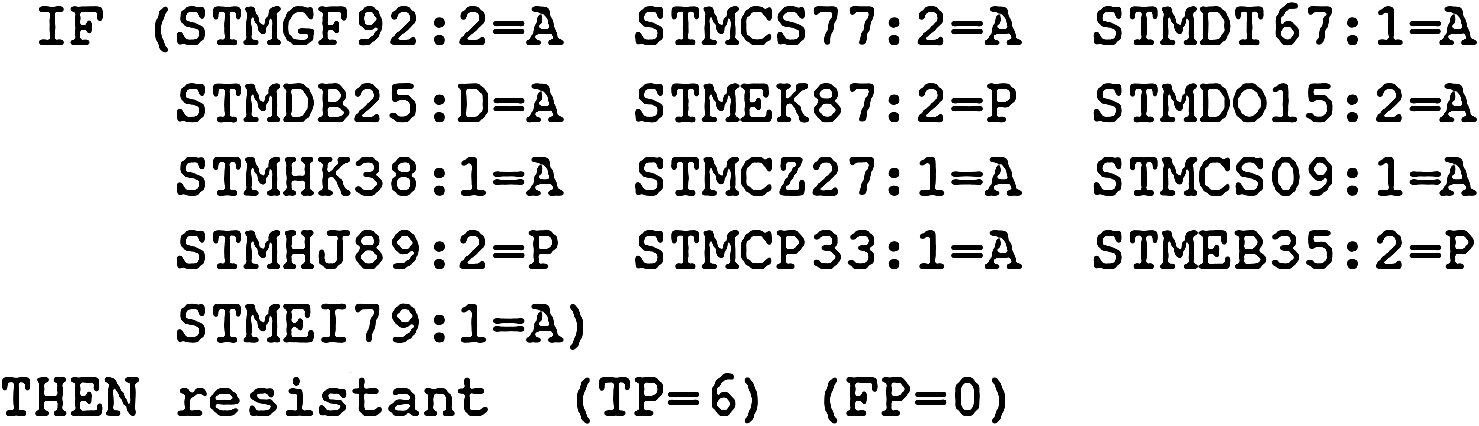
A rule induced in Experiment 1 for class resistant, using the ± 0.3 threshold, consisting of 13 conditions.

The results are presented in Table 3 where the number of conditions in rules (i.e., genes with changed expression values) that determine the resistance class is shown as a function of the selected threshold value. Expression values of obtained rule conditions determining the resistance classes are shown in Figure 3.

FIG. 3.

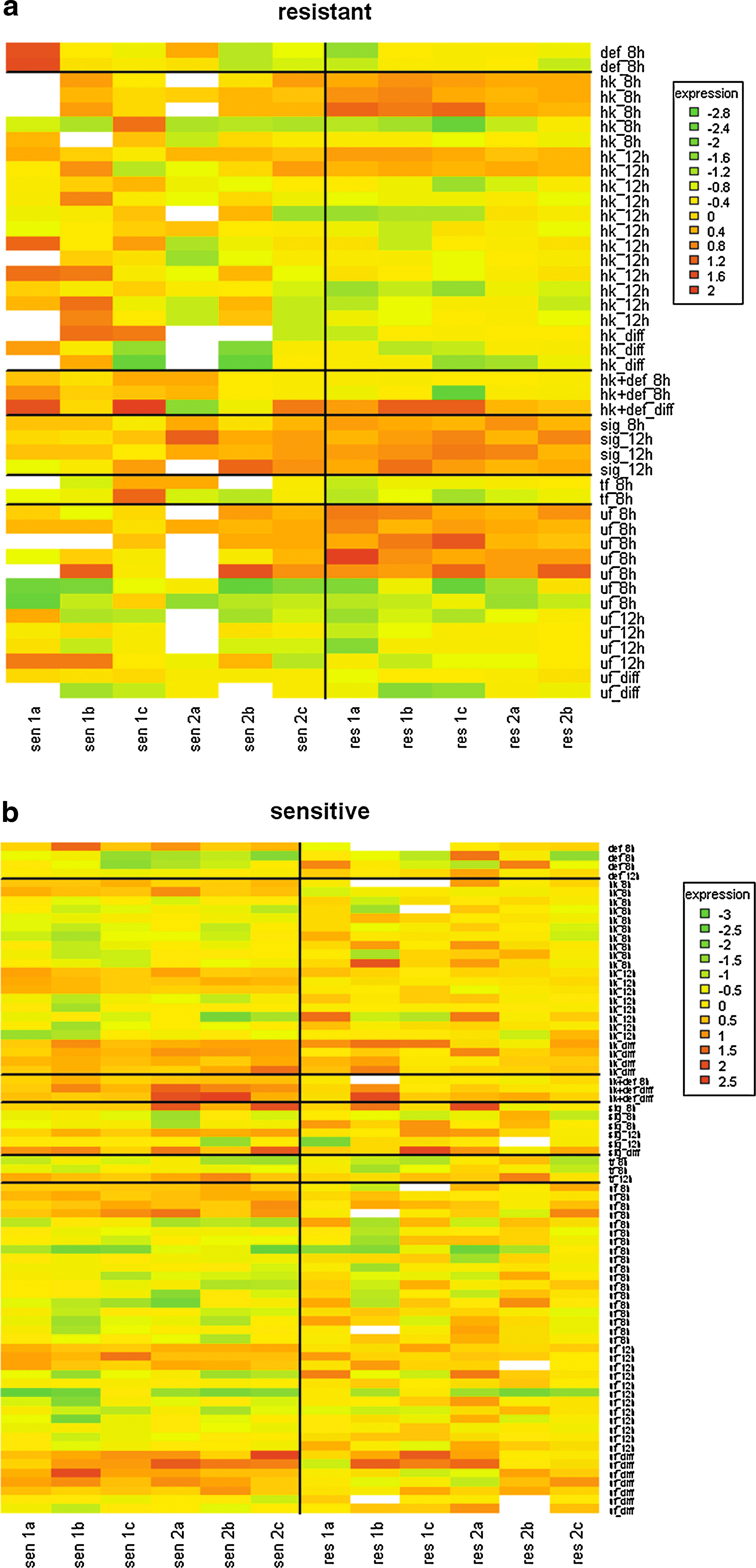
Heatmap representing genes whose expression values at a given time point determined the potato class (a) resistant or (b) sensitive for the first experiment. The expression of genes that determined a class (resistant or sensitive) is shown. Columns represent the experiment replicate: two sensitive lines (sen1 and sen2) and two resistant lines (res1 and res2) and replicates (a, b, c). Rows denote functional categories that are separated by horizontal lines (def-defence, hk-housekeeping, sig-signalling, tf-transcription factors, uf-unknown function and their combinations, if present) and time postinfection (8 and 12 h). Thus, each significantly expressed gene is represented in two subsequent rows; one for each time post infection. Biological replicates are separated by a vertical line. Missing values are denoted with a white area.

Table 3.

Data Mining Results

	Offset	Class	Number of rules ORIGINAL DATA	Number of rules PERMUTED DATA
Experiment 1	± 0.2	res	44	40
		sen	75	111
	± 0.3	res	13	10
		sen	22	46
Experiment 2	± 0.3	res	206	164
		sen	58	49
	± 0.35	res	138	88
		sen	27	22

Number of rules determining class (resistant, sensitive) for the selected offset values.

To assess the method, a statistical evaluation in the form of randomization of the data was performed. The results achieved by the RelSets algorithm were validated on the same data by permuting gene names and experimental time points used in the experiment. The number of rules obtained with permuted data is presented in Table 3. Only the results determining class resistant in the second experiment were taken into account. In all the other cases (first experiment and rules determining sensitivity in the second experiment), the number of rules was in some cases too low (<50) to get a representative sample for validation of the algorithm.

Statistical analysis

The intersection of two differentially expressed gene lists derived from applying two different normalization methods on the same data was taken as a means of selecting significantly differentially expressed genes, regardless of the preprocessing method used (Rotter et al., 2008). Two hundred genes in the first experiment and 315 genes in the second were identified as differentially expressed (p < 0.05).

The first 20 differentially expressed genes, ranked by their p-values for the first experiment, are shown in Figure 4. The normalized M values within a block (here consisting of three replicates for the experiment with the same transgenic line and the same time post infection) are more similar than those between the blocks (e.g., sen1 and sen2, where sen1 and sen2 denote the first and the second sensitive line).

FIG. 4.

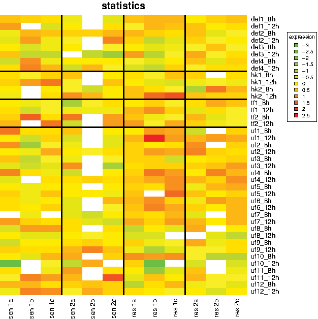
Heatmap for the top 20 differentially expressed genes for the first experiment, ranked by their respective p-values. The interaction term time × resistance was investigated. Columns represent the experiment replicate: two sensitive lines (sen1 and sen2) and two resistant lines (res1 and res2) and replicates (a, b, c). Rows denote functional categories which are separated by horizontal lines (def-defence, hk-housekeeping, tf-transcription factors, uf-unknown function) and time postinfection (8 and 12 h). Thus, each significantly expressed gene is represented in two subsequent rows; one for each time postinfection. Biological replicates are separated by a vertical line. Missing values are denoted with a white area.

Biological evaluation of obtained results

Genes that appeared in the rules and/or in the list of differentially expresed genes were assigned into functional categories using the MapMan annotation tool (Fig. 5): def-defence, hk-housekeeping, sig-signalling, tf-transcription factors, uf-unknown function, and rec-receptors.

FIG. 5.

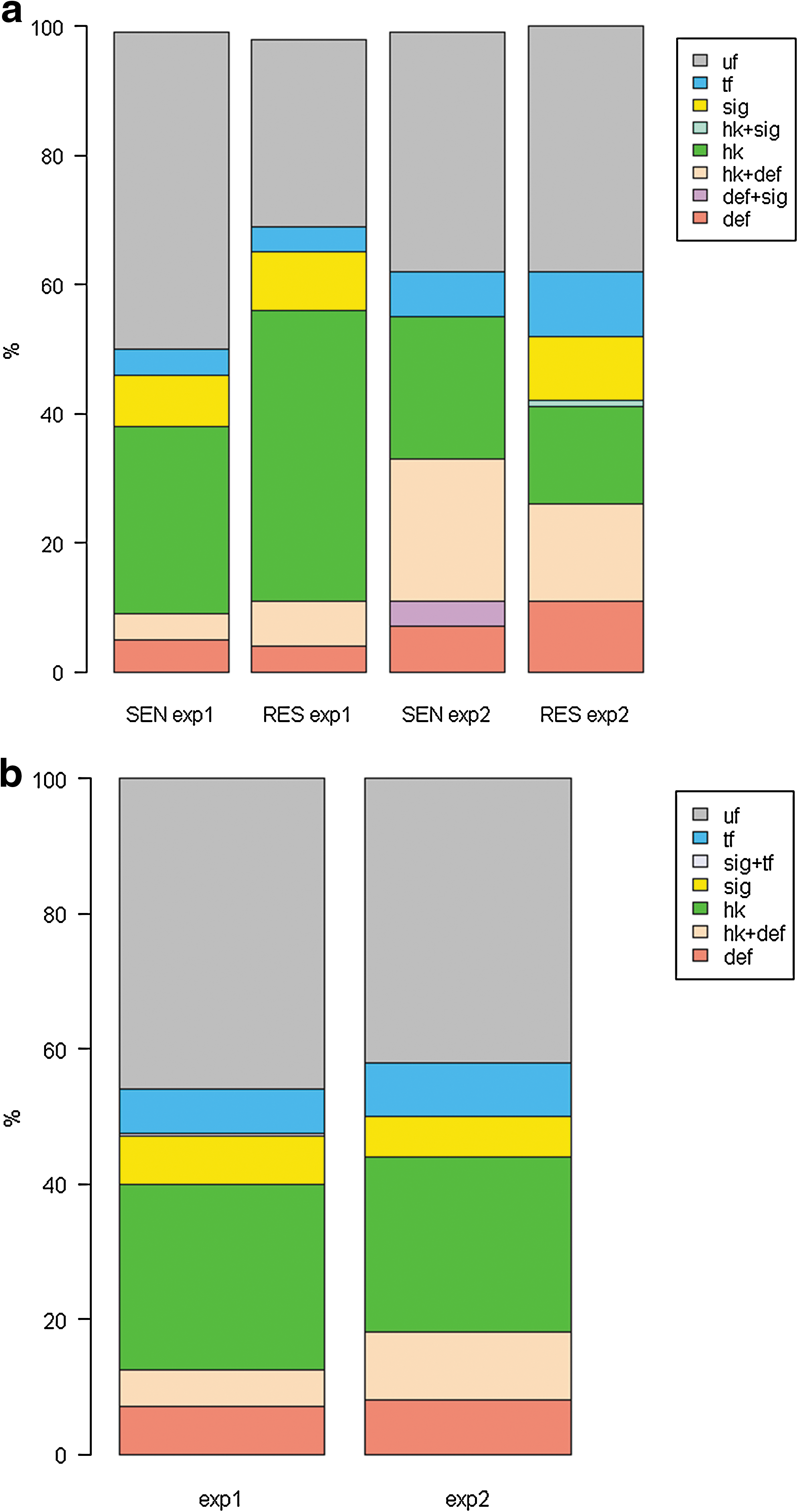
Barplot comparing functional categories (a) between conditions that determine class sensitive or resistant representing data mining results and (b) between differentially expressed genes, representing statistical analysis results for both experiments (exp1 and exp2). The percentage of genes, belonging to a category (def-defence, hk-housekeeping, sig-signalling, tf-transcription factors, uf-unknown function and their combinations, if present), compared to all genes that determine the resistance or sensitivity in an experiment or differential expression is shown. The rules (i.e., functional categories for genes that determine the resistance classes) with a threshold 0.3 for the first experiment and 0.35 for the second are shown. Note: percentages may not sum up to 100 due to rounding errors.

The genes belonging to a given functional category or their combinations, if present, were compared between classes and data analysis approaches in both experiments. We can see that the groups of genes, important for class discovery (sensitive and resistant), as well as genes whose expression changed significantly in time and between resistant types, were found as expected when analyzing plant–pathogen interactions. These are genes involved in signaling, regulation of transcription and genes with already denoted function in plant defense. Interestingly, many genes traditionally annotated as housekeeping were also present in the list of responsive genes. There was also a high percentage of genes with unknown function in all conditions analyzed. This is to be expected, because a large proportion of genes still need to have their function determined.

We have additionally applied functional classification for evaluation of rule discovery in permuted versus original datasets. The result for rules, determining resistance in the second experiment is shown in Figure 6.

FIG. 6.

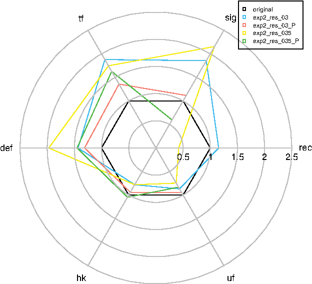
Radial plot representing validation of the RelSets algorithm by permutation. Rules determining resistance in the second experiment are shown. Offset values are marked in the figure legend (0.3 and 0.35) and permuted datasets are marked with P in the figure legend. The complete dataset (i.e., all the clones on potato microarray) was also divided to six categories (def-defence, hk-housekeeping, sig-signalling, tf-transcription factors, uf-unknown function, and rec-receptors) and is shown in black. Values on the radial plot represent percentages of category assignment in a rule compared with the original dataset. Hence, values for the original dataset are always 1. The value of 2, for example, means that for a certain category, the percentage of rules determining class resistant compared with the distribution of genes in the same category in the complete dataset was twice as high: for example, def category represented 11% of the original dataset, whereas rules obtained for Experiment 2 represented almost 23% of the categories.

Discussion

The usability of the new data mining approach was demonstrated on two experimental datasets. The tool was shown to be useful in combination with statistical analysis to add another perspective into the biological interpretation of microarray data. Using data mining enables conjunctions of conditions to be found (i.e., underexpression or overexpression of a gene after at a given time point) that are characteristic for a given class (in our case, resistant and sensitive potato plants). Several conditions that determine the class were constructed by the data mining algorithm (see Table 3). If the purpose was to select a few target genes that differ in their expression after a given time, to separate the target classes (in our case sensitive and resistant potato plants) or even define target genes for diagnostics, then a higher threshold is advised (in our case, 0.3 for the first experiment and 0.35 for the second one). This would result in a smaller number of conditions, which is more convenient, from the practical point of view of diagnostics. Data mining applications for diagnostics have been described before (Kovalerchuk et al., 2000). If the purpose of the analysis were, say, of a descriptive nature, that is, determining genes and their expression that sufficiently differentiates between two classes, then a lower threshold (0.2) should have been chosen to be able to put the conditions in a broader biological context. The threshold is preferably chosen in such a way that a reasonable number of conditions are generated, thus avoiding the issue of interpretation complexity. On the other hand, a high threshold would also pose the danger of lower reliability and robustness of the results. The choice of a threshold value is also important when accounting for the variability of the data. A higher threshold leaves less room for variable data. The only variability that is not allowed is the alternation of the signs of the M values (positive/negative M values).

Because we wanted to use the data mining (RelSets) results in a descriptive manner, a lower threshold yielding more conditions in rules (i.e., genes whose expression over time determines class sensitive or resistant) was chosen (see Table 3) to complement the results obtained using the statistical approach.

It is again important to emphasize that the data mining algorithm does not take into account the variability of data but the consistency of the result, even when variable data are represented; all replicates needed to be of the same value after discretization (P or A), because the false positive rate was set to be zero. From a biologist's perspective this is an advantage, because biological data is highly variable and sometimes information is lost due to high coefficient of variation between replicates. When discretizing data, its variability is not considered, rather the consistency of the results (i.e., comparison of the same discretized values for a particular example).

The number of biological replicates per experiment was three to four (see Fig. 1), which is the case with many microarray experiments. That is why true positive rate was set to 100%. In the cases where more replicates would have been made per experimental condition, the same true positive rate would have been chosen for, for example, highly accurate determination of genes with putative diagnostic meaning (determining a specific class). For descriptive purposes, in the case of many biological replicates, a lower true positive rate could also have been chosen.

We have also inspected the results to find genes that were part of data mining (RelSets) rules for determining both classes. In other words, we have checked if a gene was found to be important for class differentiation in both sensitive and resistant plants. Finding genes that were important for determining both classes is of great interest, because those might be the genes most connected with the biological question under study. For the first experiment, using a lower threshold of 0.2, one such gene, STMER65, involved in callcium signalling (sig category) was found. The upregulation of this gene 12 h postinfection determined class “resistant,” whereas downregulation of this gene 8 h postinfection and the upregulation of the difference between the two time points determined the class “sensitive.” If we take into account that 43 different genes determined class resistant and 71 different genes determined class sensitive, the joint probability of the same gene determining both classes in this case would be 0.0003. This shows that this particular result would highly unlikely be present by chance. The word different was highlighted because 43 different genes but 45 different features (see Table 3) costructed the rule for class resistant. In the second experiment, three such genes were found regardless of the threshold. The calculated joint probability for this happening by chance is <8 × 10⁻¹⁰ for both offsets, which again confirms that it is highly unlikely that the same result would have been found by chance. The first two genes, STMCQ55 (aspartate proteinase inhibitor) and STMCN85 (involved in secondary metabolite biosynthesis), belong to the def category, whereas the third one, STMHZ80 (RING zinc finger protein), belongs to the hk + def category. The class resistant was determined when the first two genes were upregulated in the difference of the two times, whereas the third one was absent 12 h postinfection and in the difference of the two times. Class sensitive was determined when all three genes were downregulated 30 min postinfection.

RelSets algorithm was validated by permuting clones and experimental time points. We expected that the permuted results would have resembled the original dataset (i.e., the percentage of clones of a certain category would be similar to 1, see also Fig. 6). In fact, for permuted dataset with different offset values (red and green plots on Fig. 6), the shape of the plot was similar to the complete experimental dataset (in black), except for the rec category, which originally includes in fact a very low percentage of genes (1.5%) and thus some deviations were to be expected. Moreover, as expected, results for experimental datasets (blue and yellow plots) resemble each other more than they resemble permuted dataset or the original. This is especially true for categories that play an important role for biological interpetation of the results of the experiment conducted, that is, genes, belonging to the signalling and defence category. Also, it was expected that all results (rules determining a category in the original and permuted datasets) had a similar percentage of genes, belonging to the housekeeping and unknown function categories, as they consist of the majority of the genes in all the datasets (>70% in each case), and thus are all around 1 in the radial plot (Fig. 6), similar to the original values. From a biological viewpoint, the genes, that constructed the rules were not so easily interpretable in the permuted datasets as were the “true” experimental datasets (data available upon request). Similar conclusions can be drawn for the other experimental datasets (rules that determine sensitivity in Experiments 1 and 2 and rules that determine resistance in Experiment 1). However, these datasets did not contain sufficient number of rules (<50) to be able to confirm the validation results.

When performing microarray experiments, several biological questions are asked. Sometimes the question can be to find differences between two classes of organisms tested. That can be normal versus infected tissue, wild-type versus mutant organisms, etc. Looking at the genes whose expression differes significantly between the two tested classes gives a global overview of the differences between the groups. When another factor is added to the experimental design, more complex biological questions can be answered. In our case, where two factors were tested (time and virus sensitivity), statistical analysis for the interaction term pointed to the genes that exhibited a significant change in time and between sensitivity types. We additionally tried to establish conditions that differentiate between virus sensitive and virus resistant plants. This answers a different biological question from the one addressed by statistical analysis. Here, the biological question is to find the genes and their expression in time (upregulated or downregulated) that determine the sensitivity or resistance in plants.

In conclusion, data mining and statistics, as applied in our experiments (i.e., RelSets algorithm and 2 × 2 experimental design, respectively), differ at one point when analyzing microarray data: the biological question asked. Statistics is to be preferred when it is important to know the genes that are differentially expressed under a given treatment, to focus on a more or less complex biological interpretation. However, when the goal is to determine the genes (and their expression) responsible for defining the class variable (in our case, resistant and sensitive potato cultivars), data mining with discretized values using the RelSets algorithm is appropriate. When dealing with the task of finding specific genes of interest, both types of analysis are very useful for (1) describing a biological system and its differences under different conditions, (2) helping to determine target genes for further analysis (real-time PCR or enzyme activity), (3) leading to formation of new biological hypotheses that would have to be confirmed in separate, independent experiments, and (4) possible future diagnostics of unknown samples. The appropriate experimental design and analysis will depend on the biological question being asked.