Ultradian Hemodynamics and Autonomic-Central Nervous System Activity During Sleep: A Pilot Study with Insights for Hypertension

Abstract

Introduction:

Left stroke work index (LSWI) and stroke systemic vascular resistance index (SSVRI) were compared with an ultradian rhythm of the autonomic nervous system (ANS) called the nasal cycle (NC). LSWI measures myocardial contractility and SSVRI measures after load. Mean arterial pressure (MAP) versus stroke Index (SI) has been proposed to be a useful diagnostic for the pharmacological treatment of hypertension. The NC exhibits with an ultradian rhythm in the “hourly like” range of alternating dominance of airflow through the two nostrils and is a marker of alternating lateralization of ANS activity throughout the periphery that is tightly coupled to the ultradian central nervous system (CNS) rhythm of alternating cerebral hemispheric dominance.

Methods:

Beat-to-beat measures of MAP versus SI were plotted over the sleep night in three healthy male subjects, each with three consecutive nights of sleep. The spectral time series analysis for LSWI, SSVRI, and the NC were compared, along with previously reported values for other ultradian measures in healthy adults during sleep and waking rest.

Results:

LSWI, SSVRI, and the NC have significant power in bins with periods at 280–300, 105–140, 70–100, and 40–65 min. The greatest spectral power is in longer periods. The NC also had a significant peak at 215–270 min. No significance for LSWI, SSVRI, or the NC was observed at 145–160 or 165–210 min.

Discussion:

These results suggest that LSWI and SSVRI are coupled to the NC and other ultradian rhythms regulated by the hypothalamus. MAP versus SI shows high variability and supports the importance of long-term sampling for the diagnosis and pharmacological treatment of hypertension. In addition, it is known that the yogic technique called unilateral forced nostril breathing can alter ANS, CNS, and the cardiovascular system. We expand here on the dynamics of hemodynamic states, and potentially how they may be altered to improve health.

Introduction

Thirty-two percent of noninstitutionalized adults in the United States, 20 years of age and older, as reported for the years 2003–2006, have hypertension, and there are 40.5 million ambulatory care visits per year with hypertension as the primary diagnosis. ¹ In 2004, ² it was reported that “about 50 million Americans require some form of treatment for hypertension,^3,4” and the prevalence estimates worldwide is 1 billion, and about “7.1 million deaths per year are attributable to hypertension. ⁵ ” The World Health Organization (WHO) also reported that “suboptimal blood pressure >115 mmHg systolic blood pressure (SBP) is responsible for 62 percent of cerebrovascular disease and 49 percent of ischemic heart disease” and it is the “number one attributable risk factor for death throughout the world. ⁵ ”

The WHO also reports that while 70% of individuals are aware of their condition, only 59% are being treated, and only 34% of cases are controlled with levels below 140 mmHg SBP and 90 mmHg diastolic blood pressure (DBP). ⁵ Stroke-related deaths are not declining significantly, and hypertension-associated heart failure and hypertension-associated end-stage renal disease continue to increase, and “uncontrolled hypertension clearly places a substantial strain on the health care delivery system. ² ” “Current control rates for hypertension in the United States are clearly unacceptable. ² ” These facts remain despite the introduction of many new antihypertensive drugs over the last two decades. The need for improved treatment of hypertension cannot be argued.

Preliminary data suggest that treating hypertension using both mean arterial pressure (MAP) and stroke index (SI) may lead to a more effective treatment strategy^6–13 instead of the current approach that only employs measures of MAP. In addition, the current standard for assessing hypertension usually employs only one or perhaps the average of three measures of blood pressure over 10 min. The normal endogenous rhythmic Mayer wave fluctuations in the frequency range of 0.1 to 0.01 Hz, the “hourly” ultradians, and the circadian rhythms are not considered in the standard office visit assessment.

Previous multivariate studies of ultradian rhythms during waking rest in normal healthy human adults demonstrate that the cardiovascular, autonomic, neuroendocrine, and fuel regulatory systems (insulin) are tightly coupled.^14–16 A waking study in healthy resting adults has shown that the lateralized ultradian rhythm of the autonomic nervous system (ANS) called the “nasal cycle” (NC) is also tightly coupled to the central nervous system (CNS) lateralized ultradian rhythm of alternating cerebral hemispheric activity as measured by electroencephalography (EEG). ¹⁷ And a more recent sleep study on healthy humans also shows a tight coupling of the NC and Left-Right EEG power, ¹⁸ further demonstrating the lateralized ANS-CNS coupling.

Earlier reviews of the hourly ultradian rhythms of the ANS and CNS^19,20 suggest that the temporal “Basic Rest-Activity Cycle” (BRAC) model proposed by Kleitman ²¹ (reviewed ²² ) are better understood by incorporating the lateralized rhythms of the ANS and CNS. More recent reviews with newer results also elaborate on this new model for understanding psychophysiological states during both waking and sleep.^14,23

The NC is a unique, well-studied, but not widely known phenomenon that exhibits as a lateralized autonomic rhythm. Kayser first documented the NC in 1889 ²⁴ and later described it as an “alternation of vasomotor tone throughout the periphery on the two sides of the body. ²⁵ ” It has been observed in all mammals studied. The NC exhibits as the alternating congestion and decongestion of the two nostrils in which vasoconstriction in one nostril is simultaneously paralleled by vasodilation in the other. The mucosa of the nose is densely innervated with autonomic fibers and the dominance of sympathetic activity in one nostril produces vasoconstriction in the turbinate, while the contralateral nostril expresses a simultaneous dominance of parasympathetic activity causing relative swelling. ²⁶ A 1978 study of 50 human subjects during waking over about 7 h with rhinometric pressure sampling about once a minute found a mean duration of 2.9 h ranging from 1 to 6 h. ²⁷

Kahana-Zweig et al. ²⁸ more recently used state-of-the-art instrumentation to record from 33 right-handed healthy subjects (18 F, mean age = 30.3 ± 9.9 years) on a single day with a daily routine pattern, including sleep, for 24 consecutive hours. They continuously measured left and right airflow at 5.5 Hz, using two highly sensitive pressure sensors. Their findings for cycle times were that “subjects spent slightly longer in left over right nostril dominance (left = 2.63 ± 0.89 hours and right = 2.17 ± 0.89 hours, t(32) = 2.07, p < 0.05), and cycle duration was shorter in wake than in sleep (wake = 2.02 ± 1.7 hours and sleep = 4.5 ± 1.7 hours, t(30) = 5.73, p < 0.0001).”

The NC literature reports the same uncertainty, wobble, nonstationarity, and intermittency that are common with the other ultradian phenomena. ¹⁵ The coupling of the ANS and CNS during waking rest has also been demonstrated during sleep. ¹⁸ This finding broadens our understanding of the physiology of sleep and waking states.

The purpose of this study was to observe the relationship and variability of left stroke work index (LSWI) and stroke systemic vascular resistance index (SSVRI) during sleep with the NC in normal healthy adults, and to compare any ultradian in LSWI and SSVRI with ultradians during waking rest. In addition, this study is an extension of the prior study ¹⁸ that now helps to broaden our understanding of hemodynamic states, especially in relationship to the NC and CNS ultradian rhythm. LSWI parallels the total myocardial contractility and SSVRI represents the major component of the afterload. In addition, the variability of MAP versus SI was a major focus of interest here since any variability of this parameter potentially has major implications for its utility as a therapeutic parameter for the diagnosis and treatment of hypertension.

Methods

Subjects

Three unmedicated healthy adult males (ages of 33, 44, and 48) were paid volunteers (Note: more details for this Methods Section are provided in Ref. 18). Subjects were nonsmokers, within normal weight and height ranges. Subjects participated for three consecutive nights. This study conformed with the Helsinki Guiding Principles for Research Involving Humans and was approved by the University of California San Diego Human Research Protections Program. All subjects signed a consent form after the study was explained.

Equipment

A Sleeptrace 2000/32 Polysomnographic System (International Biomedical, Inc., Austin, TX) was used to simultaneously collect data for all systems on line for the cardiac biothoracic impedance measures, blood pressures, and left and right nostril airflows. Beat-to-beat cardiovascular impedance parameters (SI, cardiac output [CO], and heart rate [HR]) were measured using a BoMed NCCOM7 Noninvasive Cardiac Monitor (Cardio-Dynamic International Corp., Irvine, CA). The Finapres Continuous Blood Pressure Monitor NIBP 2300 (Ohmeda, Boulder, CO) was used to measure beat-to-beat measures of SBP, DBP, and MAP.

Experimental procedures

The subjects were admitted to the study between 6:00 and 8:30 p.m. and each subject was run for three consecutive nights (Tuesday, Wednesday, and Thursday). The recording and attempt to sleep started between 10 p.m. and midnight at the request of the subject with lights off. The subjects were recorded in the Clinical Research Center unit of the University of California, San Diego Medical Center. The head of the bed and the region under the knees were slightly elevated to help prevent the subject from turning during sleep. No subject moved from the supine position during the recording. The left arm was immobilized on a pillow next to the side of the subject to keep an equal level between the recording finger and the heart to eliminate pressure changes due to shifts in body position.

Analytical and data processing methods

A typical 6-h record of the NC had 86,400 measurements (4 Hz) from both the left and the right respiratory signals. The left and right signals were converted to absolute values and then a left minus right value was obtained and smoothed using a moving average of over 20 points. The NC values calculated throughout the article are all left minus right using arbitrary electronic units. The beat-to-beat mode was used for the BoMed impedance cardiodynamic monitor and the Finepres Monitor.

LSWI (1) and SSVRI (2) were calculated according to the following formulas [10], [11]:

where x(i) = SI mL and y(i) = MAP Torr for each time point i

Here, LSWI, SSVRI, and the NC were subjected to time series analysis. Preliminary results for the rhythms and time series spectral analysis for LSWI, SSVRI, and the NC were previously reported, ²⁹ and an earlier publication ¹⁸ reported the time series analysis values for the same sleep records for 10 additional parameters: CO, SI, SBP, DBP, MAP, HR, hemoglobin-oxygen saturation measures (SAO2), left hemisphere power EEG (LEEG), right hemisphere power EEG (REEG), and left–right hemisphere power EEG (LREEG).

The “Fast” Orthogonal Search method (FOS) of Korenberg, a linear approach for the identification of nonlinear systems,^30–34 was applied here to the time series data using the methods as reported earlier.^15–17,35 FOS can model a time series history as a series of sinusoidal features, which, unlike the standard Fourier series, is not necessarily harmonic (commensurate). FOS selects features in the decreasing order of their ability to account for fractions of total variance. See additional details for the FOS analysis in Ref. 18.

Results

This article presents the FOS time series analysis for the beat-to-beat measures of LSWI, SSVRI, and the 4 Hz NC measures. Before FOS analysis, the parameters were first detrended for circadian components and smoothed using a moving average of 20. The earlier reported data were also detrended for circadian components and smoothed for the 3-sec root mean square measures for L-REEG, LEEG, and REEG; and the beat-to-beat cardiac impedance parameters (SI, HR, and CO), Finapres blood pressure measures (SBP, DBP, and MAP), and SAO2. ¹⁸ In addition, the entire nights of record are presented for the beat-to-beat measures for MAP versus SI, and the variance over the sleep night is broad.

Selection of period ranges

Previously, ¹⁸ we visually inspected a profile of the FOS data that included both the means of power for each period and the sums of total power for each period when all the 11 parameters (not including LSWI and SSVRI) for each of the three subjects were collapsed over the three nights of data (9 records) to produce a single power spectrum profile. Upon visual inspection, we observed that seven primary ranges or bins with periods were present. These seven bins were at 280–300, 215–275, 165–210, 145–160, 105–140, 70–100, and 40–65 min. These bins were similar to our waking study and are also those consistently reported by others in the ultradian literature for many of these variables. ¹⁵ In the earlier waking-resting state study^15,16 we observed five bins for consideration; 220–340, 170–215, 115–145, 70–100, and 40–65 min.

Inter-individual FOS analysis

The composite spectral plots of the FOS analysis for the NC, LSWI, and SSVRI for the three subjects for all three nights are shown in Figure 1.

FIG. 1.

This spectral density plot shows the fast orthogonal search time history analysis of the NC, LSWI, and SSVRI for the power distribution, or sum %TMSE after detrending of data, independent of subject and night. Each spectral plot combines three subjects for three consecutive nights per subject. Therefore, nine power spectrums are summed to produce one profile for each of the NC, LSWI, and SSVRI. LSWI, left stroke work index; NC, nasal cycle; SSVRI, stroke systemic vascular resistance index; TMSE, total mean square error.

Table 1 gives the prevalence of a significant peak for the NC, LSWI, and SSVRI for the 20-min wide bin of 280–300 min, the 55-min wide bin of 215–270, the 45-min wide bin of 165–210 min, the 15-min wide bin of 145–160 min, the 35- min wide bin of 105–140 min, the 30-min wide bin of 70–100 min, and the 25-min wide bin of 40–65 min. Chi-square analysis (two tailed) was used to determine if the frequency of occurrence of different peaks was significant across subjects for each parameter. ³⁶

Table 1.

Peak Prevalence for the Major Period Ranges for Three Subjects for Three Consecutive Nights of Sleep for the Nasal Cycle, Left Stroke Work Index, and Stroke Systemic Vascular Resistance Index

	40–65	70–100	105–140	145–160	165–210	215–270	280–300
NC	9*	9*	7*	0	2	5**	7*
LSWI	9*	6*	5*	1	3	4	8*
SSVRI	9*	8*	6*	1	3	4	4*

The columns for 40–65, 70–100, 105–140, 145–160, 165–210, 215–270, and 280–300 values are in minutes. Around 0.40% is the cutoff for %TMSE used to determine occurrence of a peak in a period range; the number tells how many subjects have at least one peak at >0.40% TMSE. ^*Indicates significance of peak prevalence at p < 0.01 (two-tailed chi-squares), or ^**p < 0.05 (two-tailed chi-squares). The maximum possible number here is 9 for the NC, LSWI, and SSVRI.

LSWI, left stroke work index; NC, nasal cycle; SSVRI, stroke systemic vascular resistance index; TMSE, total mean square error.

Table 1 lists the number of times that these periods are found for LSWI, SSVRI, and the NC when a minimum of 0.4% of the total mean square error (TMSE) is found for at least one period in that peak range. The 0.4% level is a value that is statistically above the background noise level when the time series is randomly shuffled and it is considered to be “physiologically significant.”

The TMSE of 0.4% is based, for example, on any one of the possible 3 peak values that can be identified at the three 10-min interval measures (280, 290, and 300) in the bin at 280–300 min, the 9 peak values of 215, 220, 225, 230, 235, 240, 250, 260, and 270 between 215 and 270 min, the 10 values between 165 and 210, the 4 values between 145 and 160 min, the 8 values between 105 and 140 min, the 7 values between 70 and 100 min, and the 6 values between 40 and 65 min, all at 5-min intervals.

The 0.4% is not based on the TMSE sum of neighboring peaks. The cutoff value of 0.4%, although very low, is still conservative, since frequently, there is significant activity at several neighboring values that are “shoulders” of the major peak. Much of the power for these parameters occurs in the Mayer Wave region of 0.1 to 0.01 Hz and over such long intervals of recording, the “hourly like” component of power is thus significantly reduced. The NC, LSWI, and SSVRI all show significant peaks with p < 0.01 in the bins at 280–300, 105–140, 70–100, and 40–65 min. No significance was observed in the 165–210- or 145–160-min bins. Only the NC shows significance in the 215–270-min bin at p < 0.05.

Profiles of individual parameters

Figures 2 and 3 show the time series plots of the NC, LSWI, and SSVRI for two sleep nights (subject 1 “FKF” for sleep night 1 and subject 3 “SMT” for sleep night 2), out of the total nine sleep nights. The time series as presented in this study is before the detrending that was used to eliminate the circadian component for the “hourly like” FOS analysis.

FIG. 2.

The primary time series data for subject 1 on night 1 (designated as “FKF”) are plotted from top down without detrending for the NC (left minus right nostril dominance with smoothing for every 1000 points), LSWI (with smoothing for every 500 points), and SSVRI (with smoothing for every 500 points). The scaling is adjusted for each to maximize the visual appearance of the fluctuations. The x-axis is in seconds for 5.83 h. The y-axis values for the left minus right NC measures at 4 Hz are in arbitrary electronic units related to differential thermistor activity. Data above the midline indicate left nostril airflow dominance. Data for LSWI and SSVRI are based on beat-to-beat measures and the y-axis is given in their respective units of measures. LSWI units = dyn × sec × cm⁻⁵ × m², SSVRI units = g × m/m².

FIG. 3.

The primary time series data for subject 3 on night 2 (designated as “SMT”) are plotted from top down without detrending for the NC (left minus right nostril dominance with smoothing for every 1000 points), LSWI (with smoothing for every 500 points), and SSVRI (with smoothing for every 500 points). The scaling is adjusted for each to maximize the visual appearance of the fluctuations. The x-axis is for 4.78 h for subject 3 SMT. The y-axis values for the left minus right NC measures are in arbitrary electronic units related to differential thermistor activity. Data above the midline indicate left nostril airflow dominance. Data for LSWI and SSVRI are based on beat-to-beat measures and the y-axis is given in their respective units of measure. LSWI = dyn × sec × cm⁻⁵ × m², SSVRI = g × m/m².

In these figures, the NC is presented with additional smoothing compared to the time series when they were analyzed with FOS. These figures present the data using a rolling average of 1000 for the NC, and 500 for LSWI and SSVRI. This smoothing helps to more clearly demonstrate the low frequency “hourly like” component relationships and coupling among the parameters. While LSWI and SSVRI appear to have their “hourly like” component positively in phase with each other in both nights, the “hourly like” component of the NC and LSWI appears to be inversely coupled. In some regions, the NC and SSVRI appear positively in phase, and in some, they appear antipodal with each other.

However, in the sleep night of subject 3 (SMT), the full night of the NC and SSVRI appears inversely coupled and antipodal. When subject FKF is left nostril dominant, LSWI has a lower value compared to the right nostril dominant region where LSWI exhibits with a higher value of measure. With SMT, when the NC is right nostril dominant, LSWI shows a relative increase in value. In addition to a possible direct positive, negative, or nonsignificant relationship, there is the possibility of phase lagging even when coupled systems like the ANS and cardiovascular system are regulated by the same pacemaker, that is, the hypothalamus. ¹⁵

Profiles of MAP versus SI

Figures 4–6 show MAP versus SI for the entire night for subject FKF. Figure 4 shows the two-dimensional array of all points. The light blue dot in the center of the points is the mean of all 21,298 values for MAP versus SI over the night. Figure 5 with a blue ellipse marks the border that includes 80% of all points. The light blue dot in the middle of the ellipse is the mean of all values over the night. The numbers along the trajectory inside the blue ellipse mark the path of evolution of the time series over the night, where each number in the trajectory is the mean of each 16.62 min of data. It is clear that the evolution is not random. Figure 6 shows a three-dimensional plot of MAP versus SI and the third dimension shows the density and number of events.

FIG. 4.

The MAP versus SI beat-to-beat measures for subject 1, night 1 (FKF), is plotted for the entire sleep night with semi-log plots. Raw measures of SI are used. These values are in milliliters per beat of the heart. Therefore, the SI measures are in integer values and this is apparent in the scattering of the plot. No smoothing, detrending, or other treatment is carried out on these data. MAP is also in untreated raw measures. The turquoise dot central to the violet points is the mean of values for the entire night of 5.83 h. The blue ellipse is drawn to show the 80% boundary for all MAP versus SI points over the night. The diagonal isolines for vasoactivity (SSVRI) are plotted in green, and the opposing gray diagonal isolines are for contractility (LSWI). The violet hexagon in the center defines the borders for normal MAP pressure and normal SI values for healthy adults during waking rest. Almost all points are outside the hexagon and show low flow and near normal to low pressure. The mean value for MAP is ∼71 mmHg and the mean for SI is ∼31 mLs/beat. MAP, mean arterial pressure; SI, Stroke Index.

FIG. 5.

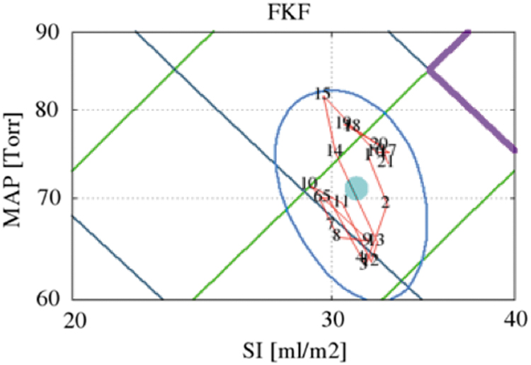
The blue ellipse is drawn to show the 80% boundary for all MAP versus SI points over the night for subject 1, night 1 (FKF). The turquoise dot shows the mean value for the entire night. The red line with numbers shows the evolution of means for every 16.62 min of data. The violet line shows a portion of the hexagon for normal ranges for Map versus SI. The means do not follow a random sequence.

FIG. 6.

The beat-to-beat plots of MAP versus SI and the number for events for each (MAP, SI) pair are shown for subject 1, night 1 (FKF). The points are almost all outside the violet hexagon and show low flow and near normal to low pressure.

Figures 7 and 8, and Supplementary Figure S1 (see in the Supplement) show MAP versus SI for subject 3, night 2 (SMT), with the same respective information presented. These plots clearly illustrate the wide variance of the MAP versus SI parameter across the night and this was the case for all nine sleep nights for the three subjects. Figures 4 and 7 also include the diagonal isolines for vasoactivity (SSVRI) that are plotted in green as they compare to the brown hexagon in the center that defines the borders for normal pressure of MAP and normal values for volume (SI).

FIG. 7.

The MAP versus SI beat-to-beat measures for subject 3, night 2 (SMT), is plotted for the entire sleep night with semi-log plots. Raw measures of SI are used. These values are in milliliters per beat of the heart. Therefore, the SI measures are in integer values and this is apparent in the scattering of the plot. No smoothing, detrending, or other treatment is carried out on these data. MAP is also in untreated raw measures. The turquoise dot central to the violet points is the mean of values for the entire night of 5.29 h. The blue ellipse is drawn to show the 80% boundary for all MAP versus SI points over the night. The diagonal isolines for vasoactivity (SSVRI) are plotted in green and the opposing gray diagonal isolines are for contractility (LSWI). The violet hexagon in the center defines the borders for normal MAP pressure and normal SI values for healthy adults during waking rest. The majority of points is within the hexagon and shows normal flow and normal pressure. The mean value for MAP is ∼73 mmHg and the mean for SI is ∼44 mLs/beat.

FIG. 8.

The blue ellipse is drawn to show the 80% boundary for all MAP versus SI points over the night for subject 3, night 2 (SMT). The central turquoise dot shows the mean value for the entire night. The red line with numbers shows the evolution of means over the night of sleep for every 13.23 min. The violet line shows a portion of the hexagon for normal ranges of MAP versus SI. The means do not follow a random sequence.

Figures 4 and 7 also show the opposing diagonal isolines for contractility (LSWI). The major difference in the plots for FKF and SMT are that the majority of points over the night for SMT is within the hexagon, and almost none is within the hexagon for FKF. The sleep night for SMT shows normal pressures and low to normal flows, and FKF shows low to normal pressures and hypo-normal flows. However, it should be noted that the hexagon borders for normal pressures and normal flows in this study are based on waking values in healthy adults.

Discussion

The analysis of LSWI and SSVRI in this study helps to further define the variation in the ultradian hemodynamic states over the sleep night, and how these two markers are coupled to the NC, an important marker of ANS, CNS, and other psychophysiological parameters. All three markers show significance at p < 0.01 for peaks in the 280 -300, 70 -100, and 40–65-min bins. However, the NC also shows marginal significance at p < 0.05 in the wider 215–270-min bin.

These results for LSWI and SSVRI are consistent with the earlier analysis, ¹⁸ which also included the NC and seven other cardiovascular parameters (CO, SI, HR, SBP, DBP, MAP, and SAO2) and three parameters of CNS activity (LEEG power, REEG power, and L-REEG power), which had similar power spectral profiles across subjects with significance of p < 0.01 (chi-square, two tailed) for peak activity in the four major bins of 280–300, 105–140 (except LREEG, LEEG, and HR), 70–100, and 40–65 min. In the previous analysis, ¹⁸ four parameters (HR, LEEG, REEG, and SAO2) also showed marginal significance at p < 0.05 in the 145–160-min range, and two parameters (NC, p < 0.05; REEG, p < 0.01) also show significance in the wider 215–270-min range.

Overall, the dominant bins were 280–300, 105–140, 70–100, and 40–65 min. These results are also consistent with a waking study^15,16 that included (except EEGs and SAO2) normal healthy adults for all of these parameters and 14 others with simultaneously venous sampling of both arms for luteinizing hormone (LH), adrenocorticotrophin hormone (ACTH), insulin (INS), both left arm norepinephrine (LNE) and left arm epinephrine (LE) and right arm norepinephrine (RNE) and right arm epinephrine (RE) and mean arm values of norepinephrine (MNE) and mean arms values for epinephrine (ME), and left minus right values for norepinephrine (LRNE) and epinephrine (LRE), respectively, and three additional cardiac impedance measures (ventricular ejection time [VET], ejection velocity index [EVI], and thoracic fluid index [TFI]).

The time series history analysis for the following 22 variables in the waking study with healthy adults—NC, LH, ACTH, INS, SBP, DBP, MAP, TPR, LE, LNE, RE, RNE, ME, MNE, LRE, LRNE, CO, TFI, HR, EVI, SV, and VET—clearly showed for most variables the predominance of significant peaks in the bins of, 115–145, 70–100, and 40–65 min. The exceptions were the absences of statistical significance for ACTH at 115–145 min, NC and LH at 40–65 min, and the epinephrines and SBP, DBP, and MAP at 115–145 min.

The blood pressure parameters during the waking study were not beat-to-beat measures, but were captured at one automated cuff measure every 7.5 min (similar to the sampling for the blood plasma parameters for the catecholamines and pituitary hormones), and perhaps would have shown rhythms in the 115–145-min bin, which were exhibited with the beat-to-beat sampled cardiac impedance variables. While all these 22 waking parameters (except TFI and HR) had some activity at 220–340 min, only the NC and LH showed significant chi-square values along with their greatest spectral power in the 220–340-min bin.

While this is a wider bin than the two neighboring bins used during the sleep study (280–300 and 215–270 min), considerably less activity was observed in this longer period domain during the waking state compared to sleep, even though both studies were of near equal length and where both used data detrended for circadian rhythms. ACTH had its greatest power in the 170–215-min bin.

The broad bin of 70–140 min is the bin of periodicity most commonly reported for the “hourly like” ultradian rhythms (reviewed^15,16). However, here this bin was analyzed as two separate components, the 105–140- and 70–100-min bins, and it was analyzed as 115–145- and 70–100-min bins during the waking study. These two bins represent the two largest of the five during the waking study in respect to the sum total of the % TMSE. These two bins also dominate during this sleep study, but the 280–300-min bin for sum total % TMSE must be included, which also existed, but to a lesser extent during the waking state, as well as the 40–65-min bin for both the sleep and waking states, but with lower % TMSE.

Therefore, this report provides further insight into how two important parameters of the cardiovascular system (LSWI and SSVRI) are also likely coupled to the ANS, CNS, neuroendocrine, and fuel-regulatory hormone systems. These results also suggest that the hypothalamus is regulating the “hourly like” ultradian rhythms.

Earlier reviews^14,19,23 present the evidence and make the case that the NC and the BRAC are coupled, whereby right nostril dominance (left hemisphere dominance) is a marker and coupled to the activity phase of the BRAC, and that left nostril dominance (right hemisphere dominance) is a marker and coupled to the rest phase of the BRAC. While LSWI and SSVRI appear to have their “hourly like” component positively in phase with each other, the “hourly like” component of the NC and LSWI appears to be inversely coupled. However, in one subject night, some regions of the NC and SSVRI appear in phase, and in some regions, they appear antipodal with each other. However, in the sleep night of the second presented subject (SMT), the full night of the NC and SSVRI appear inversely coupled and antipodal in phase.

When subject FKF is left nostril dominant, LSWI has a lower value compared to the right nostril dominant region where LSWI exhibits with a higher value. This would suggest that the value of work as measured by LSWI is higher during the right nostril activity phase of the BRAC. For the second subject presented, during right nostril dominance, LSWI shows a relative increase in value. These generalities tend to hold up in all three subjects. The tendency of greater right nostril dominance and greater values of SSVRI also tends to predominate. However, more subjects are required to confirm this tendency and how the phase shifts occur between LSWI, SSVRI, and the NC as a marker of the BRAC, psychophysiological states, including hemodynamic states.

The ultradian dynamics of LSWI and SSVRI exhibit with very wide variance over the sleep night. A similar variance is expected during waking rest and during states of activity. Since the MAP versus SI marker has recently been employed as a marker for the diagnosis and pharmacological treatment of hypertension,^6–13 it is expected that the longer the window for MAP and SI sampling, the more accurate the diagnosis would be and which medication is most suited for treatment. We encourage the use of 8–10-h beat-to-beat sampling under waking rest and during a full night of normal sleep to gain insight to this variance for this purpose.

The results of our work presented here, and the earlier report ¹⁸ included only three healthy males. Studies with females and additional males, broad age ranges, hypertensive patients, and various states of health and disease are required to gain a more accurate view of sleep stage ultradian hemodynamics and this ANS-CNS rhythm and its marker, the NC. This will provide a more clear understanding of disease states, health, and inter-system dynamics. In addition, adding an analysis of HR variability parameters would broaden the scope of this analysis. These results also give us more insight to how unilateral forced nostril breathing techniques may help to improve health and ultimately control hypertensive states and other health problems.