
Abstract
In the United States, from 1989 to 2020, there have been more than 560,000 confirmed releases from leaking underground storage tanks (LUSTs). As of March, 2022, there are nearly 540,000 active underground storage tanks (USTs) and nearly 60,000 LUSTs remaining to be cleaned up. These releases occurred from a universe of 2.5 million UST systems, storing petroleum or hazardous substances. LUSTs can contaminate surface water and groundwater, affecting both private and public drinking water supplies. For example, 42% of documented releases occur in source water protection areas—areas that hydrologically contribute to public drinking water supplies. LUSTs can contaminate soils leading to land-use restrictions and associated diminished economic value. Petroleum plumes can migrate under structures causing petroleum vapor intrusion into buildings. Contamination from LUSTs may result in deleterious effects to human health and the environment. The U.S. Environmental Protection Agency (EPA) has recently published the first national data on the locations of USTs, UST facilities, and LUSTs including all states and territories. Using this national data set in combination with the data obtained from EPAs Environmental Justice Screening and Mapping Tool (EJScreen), this article investigates whether low-income communities and communities of color are disproportionately exposed to LUSTs and potential pollution from USTs. We conducted analyses of UST and LUST density for the United States and their proximity to communities of color and low-income communities at several administrative levels using multiple spatial and statistical methods. We find that both communities of color and low-income communities are disproportionately burdened by USTs and LUSTs.
INTRODUCTION
In 1994
Among contaminants of concern to disadvantaged communities are petroleum hydrocarbons that can be released into the environment from underground storage tanks (USTs). USTs typically store petroleum products at gasoline stations and present a point-source contamination risk to groundwater, the source of roughly half of U.S. drinking water—both public and private. 3 Between 1989 and 2020, there have been 2.5 million federally regulated UST systems storing petroleum or hazardous substances in the United States. Within these systems, there have been 568,000 confirmed leaking underground storage tanks (LUSTs), illustrating that about 25% of these tank systems have had a confirmed release. This is a rough estimate, as aggregate data do not tell us if reported leaks are from a fewer number of tanks repeatedly, or one leak per tank over a given time period. 4 Presently, there are about 540,000 active USTs and 60,000 USTs remaining to be cleaned up are LUST sites. Addressing this backlog of LUST sites is a priority for Federal, state, territorial, and tribal authorities overseeing these cleanup/remediation programs.
Petroleum–hydrocarbons exist in the environment both as legacy contaminants at closed sites where residual contamination may still be present and at active LUST sites. Current contaminants at LUST sites may also be at risk of further mobilization in the future if residuals remain and site conditions change due to extreme weather or other climate-change-related events.
In the 2000 National Water Quality Inventory, 52 states, tribes, and territories reported that their major sources of groundwater contamination are USTs, septic systems, and landfills. 5 Historically, 13% of documented releases have occurred within surface water protection areas (composed of NHDPlus V 2.1 catchments located 24-hour time of travel upstream of all valid surface water source facilities) and 36% have occurred within wellhead protection areas (composed of NHDPlus V 2.1 catchments that intersect wells). Presently, 45% of active USTs and 47% of LUSTs are in wellhead or surface water protection areas. Regarding private supply, there are an estimated 267,000 private domestic wells within 1500 ft of an active LUST. 6
Benzene is a primary human health concern from fuel releases. It is a known human carcinogen, with exposures evidencing an increased risk of leukemia as well as other potential adverse effects. 7 These can include reproductive, mutagenic, cardiologic, neurological, and immunologic effects. 8 The maximum contaminant level (MCL) for benzene in drinking water is 5 μg/L, lower than the taste or odor thresholds of 0.5–4.5 and 60 ppm, respectively. 9 Fuel additives, such as ethylene dibromide with an MCL of 0.05 μg/L, may also be a concern associated with legacy sites. 10
In addition to impacts on water supplies, air emissions may be a concern. In field studies that examined benzene air emissions from gas station vent pipes using California's Office of Environmental Health Hazard Assessment 1-hour acute Relative Exposure Levels (REL), benzene concentrations exceeded the REL up to 160 m from the gas station. 11 These emission rates will be especially important in communities where fueling facilities have high volumes of product and a high density of facilities within a community.
Previous studies have shown that low income and populations of color bear a disproportionate burden from LUSTs at local and regional levels. 12 , 13 The specific definitions of terms such as “environmental justice” (EJ) and “environmental equity” have been debated for decades. 14 , 15 At a national level, Executive order 12898 set an approach to environmental justice such that; “each Federal agency shall make achieving environmental justice part of its mission by identifying and addressing, as appropriate, disproportionately high and adverse human health or environmental effects of its programs, policies, and activities on minority populations and low-income populations in the United States and its territories and possessions, the District of Columbia, the Commonwealth of Puerto Rico, and the Commonwealth of the Mariana Islands.” 16
Charles Lee, current Senior Policy Advisor for the Office of Environmental Justice at the U.S. Environmental Protection Agency (EPA), recently wrote that “A justice perspective means the prevention and mitigation of environmental harm, identifying and addressing policies and practices that contribute to disproportionate impacts, and the elimination of systemic barriers to health and sustainable communities for all people.” 17
The purpose of this article was to determine whether USTs and LUSTs are disproportionately located in or near communities of color (all people other than non-Hispanic white-alone individuals) and communities with lower economic status or income, in line with Executive Order 12898s definition of EJ. This investigation is possible for the first time at a national scale with the recent release of EPAs UST Finder, a comprehensive database of all UST facilities and reported releases for the 50 U.S. states, federally recognized tribes, District of Columbia, and territories. 18 We use the locations of USTs and LUST facilities, combined with sociodemographic data obtained from EPAs EJScreen within multiple established statistical methods to examine if low income and communities of color are disproportionately exposed to both confirmed releases from LUST sites and potential releases from active UST facilities.
DATA AND METHODS
We use proximity analysis to colocate UST and LUST locations within census block groups with demographic indicators obtained from EPAs 2020 release of EJScreen. 19 Block groups were binned based on demographic variables, and the Mann–Kendall test was applied to test for statistical significance between UST and LUST block group densities and associated sociodemographic data. A pairwise Wilcoxon rank sum test was applied to test for disproportionality of USTs and LUSTs on low-income communities and communities of color. Finally, the white to non-white ratio 20 was applied to minority and low-income variables along with tank and release densities to map distributions of inequality. We also calculated the ratio of releases to tanks to determine whether releases were occurring at disproportionate rates in low income or communities of color.
UST data
The U.S. EPA has the authority under Subtitle I of the Solid Waste Disposal Act to approve states, territories, and the District of Columbia UST programs. EPA is the primary implementing agency in Indian country. UST data maintained by the states, territories, and the District of Columbia, as well as EPA's data for Indian country, is the foundation for the UST Finder data. 21 We used three data sets within the EPA UST Finder database: UST facility locations, USTs, and LUST locations. UST facilities refer to the singular location of a facility that may have one or multiple tanks on site, such as a gas station. The UST data set references a table of characteristics of specific tanks including data on capacity, substance stored, and installation date. The UST data set is not spatial but has a many-to-one relationship with the UST facility data. Thus, tanks are geolocated based on the coordinates of their parent facility.
The LUST data set, such as the UST facility data set, represents the singular location of where a confirmed release has been reported. Locations within the UST Finder data set that were not directly provided by the delegated programs were geolocated by EPA with varying locational accuracy ranging from zip code to point address. Both active and closed tanks installed after 1969 were included in this analysis, with a street intersection geocode accuracy or better, or state-supplied coordinates (N = 1.9 million). We included releases reported after 1969 with a street intersection geocode accuracy or better, or state-supplied coordinates (N = 483,446). Both open and closed USTs, and open and closed LUSTs were included in this analysis to capture current and historical conditions.
Demographic data
Percentile minority and percentile low-income data were obtained from the 2020 release of EPAs EJScreen. Minority status is defined as the percentage of individuals in a block group who list their racial status as a race other than white alone and/or list their ethnicity as Hispanic or Latino. Low-income status is defined as the percentage of a block groups' population where the household income is less than or equal to twice the federal poverty level. 22 Data were obtained at the Census block group level, which are population-based spatial delineations, typically encompassing between 600 and 3000 residents. 23
Spatial consideration
In a meta-review of plume length studies, Connor et al. found that the upper distance of petroleum hydrocarbons from the leak/spill source at concentrations above the MCL (5 μg/L) is ∼1500 ft. 24 Using this radius of influence, UST facilities and releases were spatially joined to block groups, as well as block groups that were within 1500 ft of their locations to account for the potential for plumes to cross block group boundaries. This method ensures that potential impacts to communities from UST and LUST sites are accounted for that may not directly intersect with a block group but are within a distance where contamination can migrate.
Statistical analysis
Census block groups were split by percentile minority into 10 bins representing 10 percentile groups. This process was replicated for percentile low income. Binning by percentiles ensures the sample size for each bin is similar. Using R statistical software, we conducted the Mann–Kendall test to determine the existence and significance of a trend relationship between UST or LUST density and percentile minority or low income from sequential high to low and low to high bins. 25 , 26 We then calculated the Sens slope value to provide coefficients for probabilities across bins within each variable group to quantify the effects of increases in minority/low-income community populations on tank/release density.
The second test we used was the pairwise Wilcoxon rank sum test, which aims to quantify statistical differences between unique groups of data, in this case, block groups binned by either percentile minority or percentile low income. 27 The pairwise Wilcoxon also yields an effect size that can be thought of as an inverse pseudo r2—where an effect size of 0 indicates that the two populations are statistically identical and an effect size of 1 indicates that the two populations are completely different.
The third test we used was the white to non-white exposure ratio (hereafter “the inequality ratio”), proposed by Boyce et al.,
28
to identify areas with disproportionate densities of tanks and releases to population groups. We use percent minority and percent low income for the
“Where subscript j indexes the population group: and Xij is the share of group j in the population of [area].” 29 INEQUALITY i is derived from UST Finder data, producing variables for tanks/km 2 , and releases/km 2 . Xij is derived from the percent minority and percent low-income EJScreen demographic indicators (not binned). We conducted separate iterations for every combination of INEQUALITY i and Xij at the census tract, census combined statistical area (metropolitan area), and county levels for all 50 states, Puerto Rico, and the District of Columbia. County-level estimates are reported in the Results section, and all other results are available in the supplemental material.
Finally, we tested whether communities of color and low-income communities experience, as a proportion of their tank universe, a higher rate of reported releases than white and non-low-income communities. For every year from 1989 through 2018, we calculated the ratio of reported releases to active tanks for every block group in the United States. The average ratio of releases to active tanks for the period between 1989 and 2018 was then calculated for each block group from the yearly ratio. This yields a ratio of active tanks to releases for every block group, which is then tested with the Mann–Kendall test against binned minority and low-income percentiles to determine if minority or low-income communities have a disproportionate rate of releases compared with active tanks.
RESULTS
Binning both minority and low-income percentiles and plotting them against tank and release densities shows a positive trend: as percentile minority and percentile low-income increase, so do tank and release densities (Fig. 1). In all four panels of Figure 1, for every bin, the median density and interquartile range is greater than the previous bin. In other words, the higher the percent of people of color or low income in a community, the higher the UST and LUST density. For example, in block groups within the 0–10 minority percentile, the median tank density is 0.73 tanks/km 2 , whereas in block groups between the 90 and 100 minority percentile, the median tank density is 45.3 tanks/km 2 , a 62-fold increase.
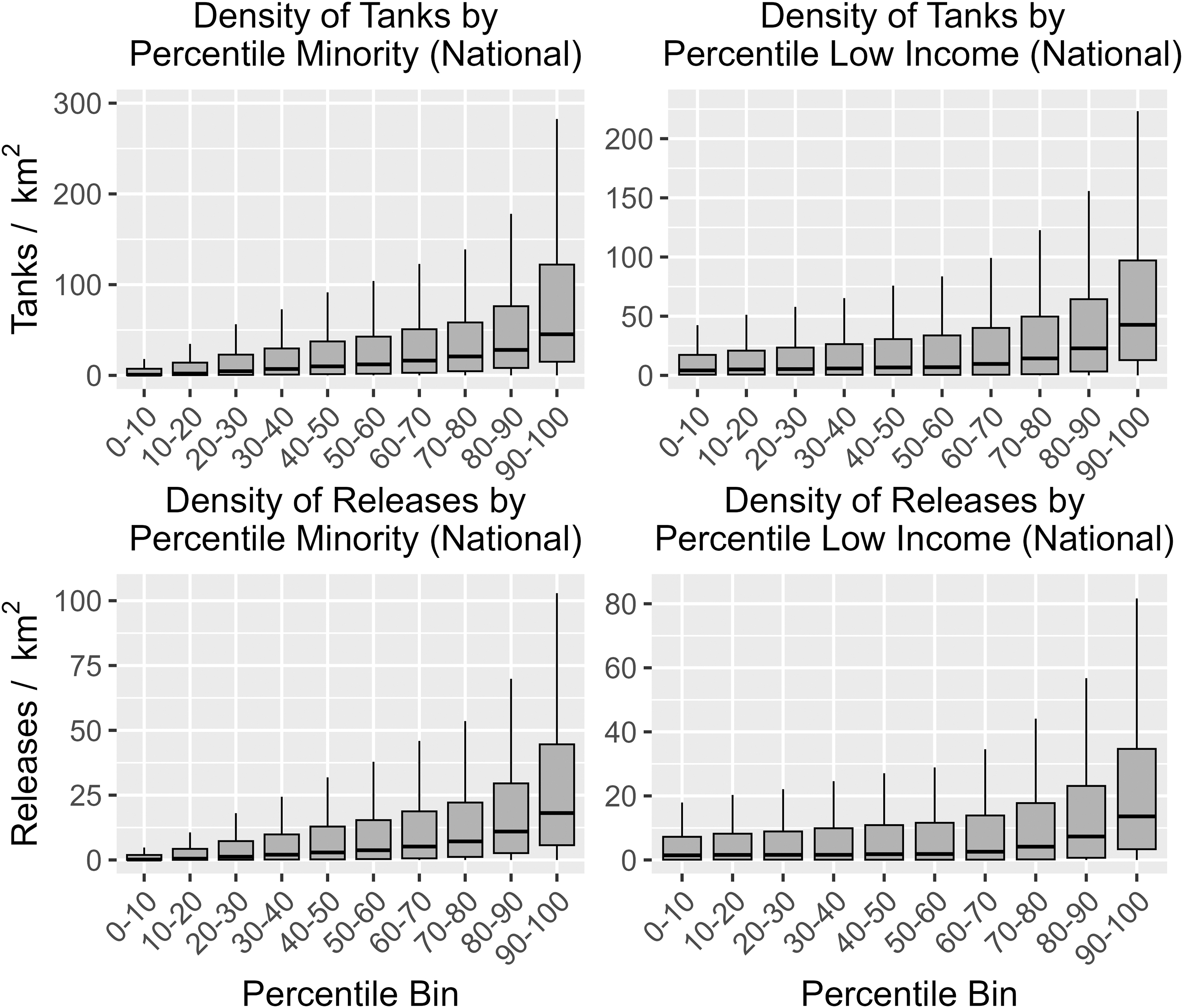
Box plot illustrating groups binned by percentile minority and percentile low income and tank and release densities.
The Mann–Kendall trend test supports the interpretation in Figure 1, showing statistical significance for all variable combinations (Table 1). The strongest trend is tank density against percentile minority (Sens slope = 3.26). The Sens slope value indicates the slope of the relationship across bins. For tank density and percentile minority, this indicates that as bins increase, tank density increases 3.26 tanks/km 2 , on average. This indicates that communities with a higher percent of non-white or low-income residents are more likely to have an UST or LUST in their community.
Results from the Mann–Kendall Test for Combinations of Tank and Release Densities, and Percentile Minority and Low Income
The pairwise Wilcoxon rank sum test shows statistically significant differences and high effect sizes between the lowest and highest percentile bins for all combinations of minority, low-income, tanks, and releases (Fig. 2). For example, a community in the 90–100 percentile of minority is much more likely to have a higher density of tanks than a community in the 0–10 percentile of minorities. Conversely, a community within the 10–20 percentile of low-income communities is likely to have a similar density of releases to a community within the 30–40 percentile of low-income communities.
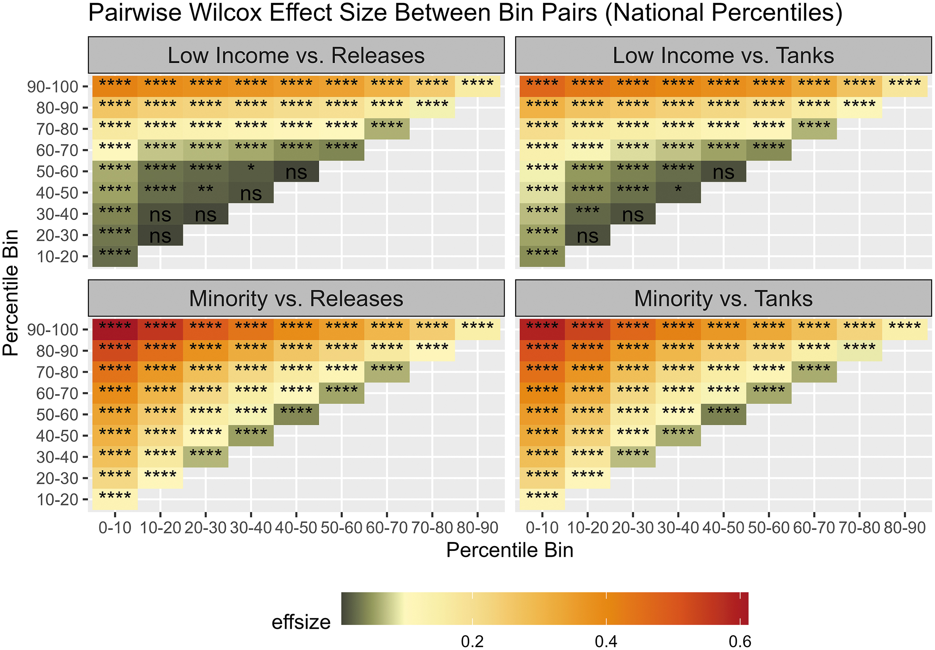
Heat map showing results of the pairwise Wilcoxon test. Percentile bins are compared on the x and y axes. Green indicates weak effect, red indicates strong effect, “****” indicates highly significant, and “ns” indicates not statistically significant.
The inequality ratios have national medians (Table 2) ranging from 0.02 (minority: releases) to 0.293 (low income: tanks). The minimum ratio values were all zero, indicating counties where tanks and releases are present only in white or non-low-income communities. Likewise, maximum values were all infinite, indicating counties where tanks and releases are only located in areas of low income and communities of color. To map areas of higher inequality to low income and communities of color, we split the inequality ratios at their national medians and combined them with tank and release densities, also split at their national medians (Fig. 3).
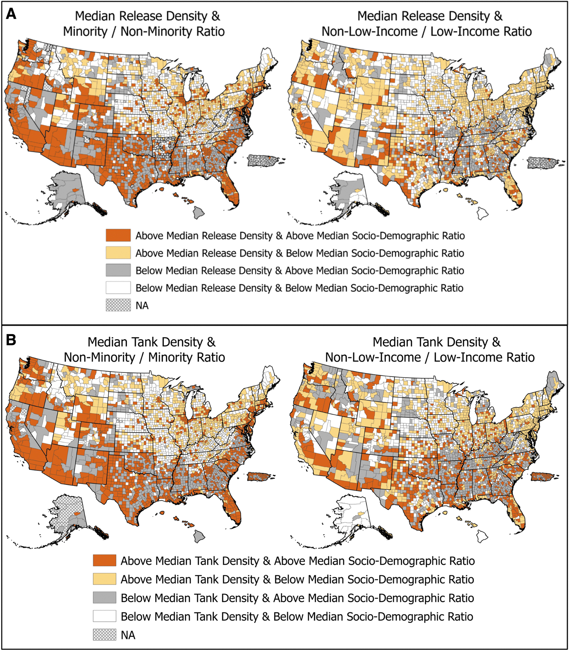
Maps showing U.S. counties above and below the national median of tank densities
Breakdown of Minimum, Median, and Maximum Values for Inequality Ratio Results
We found that there is no statistical difference between the ratio of reported releases and active USTs across minority and low-income percentiles (Fig. 4). The Mann–Kendall test showed p-values of 0.084 and 0.49, respectively, for minority and low income. Both minority and low income had slopes of 0.00. This indicates that the ratio of releases to tanks is consistent across block groups, regardless of their percentile minority or percentile low income. While this reflects equality in outcomes, in terms of rate of releases across communities, it does not account for equity regarding low income and communities of color as has been demonstrated in the Mann–Kendall and pairwise Wilcoxon tests. This relationship was also consistent when considered for each individual state (Supplemental Information).
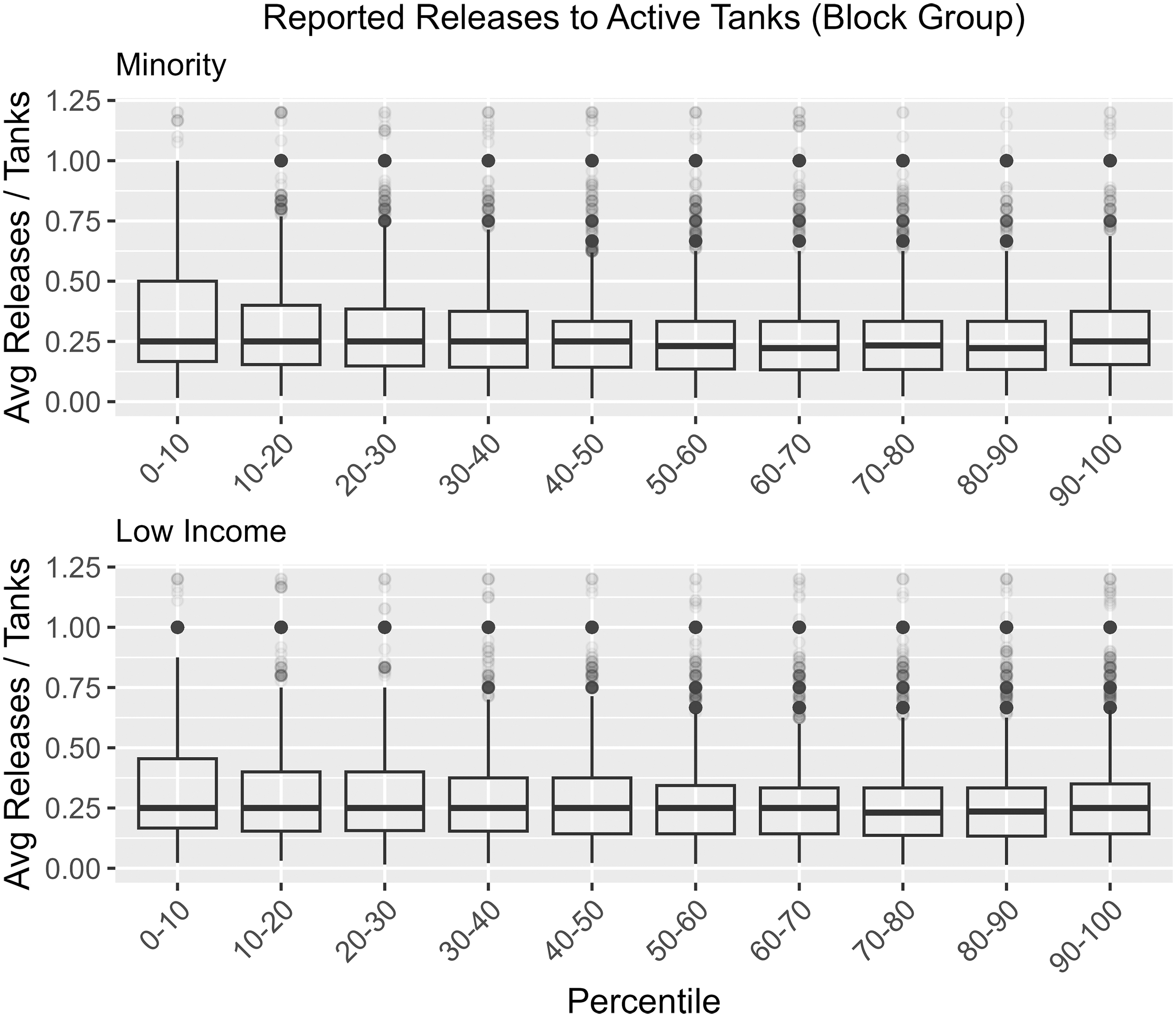
Box plots showing the average ratio of releases to tanks related to percentile minority and percentile low income.
DISCUSSION
Our results present a picture of inequality for both low-income communities and communities of color from both USTs and LUSTs. There are statistically significant trends, which support the hypothesis that as percentile minority and/or percentile low income increase, communities are more likely to have USTs and releases in or near them. The strongest trend in the Mann–Kendall test is between tank density and percentile minority. The Sens slope value dictates that on average, as you move from one percentile bin to the next highest bin, tank density increases 3.26 tanks/km 2 . The results of the pairwise Wilcoxon test support the findings of the Mann–Kendall test in that we show statistical differences between populations, represented as bins. The most significant differences and strongest effects in tank/release densities are exhibited between the highest and lowest concentrations of low income and communities of color. These findings support that if a community was chosen at random, the sociodemographic makeup of that community can provide a compelling proxy for their colocation of UST infrastructure, and vice versa.
With regard to equity at subnational scales, mapping the results of the inequality ratio allows us to discuss the spatial implications of equality at the county level. Tank densities, for example, show more inequitable distribution to communities of color combined with higher tank densities in the American south, with notable additional areas in the rest of the United States, primarily colocated within major metropolitan areas such as Chicago, Detroit, and Minneapolis. With respect to low-income communities, the pattern is somewhat more disperse, but still dominant in the south, with cities in the north such as Wichita (KS), Columbus (OH), and some rural areas across most states. The inequality ratios for releases and low-income communities/communities of color follow similar patterns as tanks.
There are some differences to note, such as Pennsylvania, which shows multiple counties with higher inequality ratios for low income and tank densities, but not for release densities. Areas in yellow and white (Fig. 3) illustrate dominantly white or non-low-income areas and are prominent across the midwestern states. While some of the patterns of inequality USTs and LUSTs locations are familiar, such as in the American south where there are higher concentrations of populations of color, there are areas that may reflect other driving forces. For example, in many areas, this relationship was most likely driven by communities that are geographically close but demographically diverse, suggesting that there are less tanks located in relatively white communities and more tanks within relatively more populations of color in the same county.
There are several reasons for a specific UST facility location—and in particular, gas stations. These include proximity to roads, traffic volume, population density, zoning, historical land use, and property value to name a few. These reasons and in particular the expansion of roads and interstates after the 1956 Federal-Aid Highway Act have serious EJ implications that relate to where tanks are located and in turn subject these communities to disproportionate risk. Wherever people drive, people also fill up their gas tanks, with tertiary consequences such as spills, accidents, explosions, and subjugation to vehicle exhaust. 30 Tanks and releases are disproportionately located in urban and inner-suburban (close to urban centers) areas, as are low income and populations of color.
While the statistics described in this article quantitatively describe the unequal burden of potential UST/LUST by varying sociodemographic groups, the inequality ratio analysis provides a geographic context where potential human and environmental health inequities are of greatest concern. These data can now be used by communities, states, and agencies to inform additional analysis and assessment concerning a range of applications, from permitting gas stations at the local level, to triaging inspections to cleanups. Additionally, tank facilities can be considered in addressing cumulative effects from other sources such as Resource Conservation and Recovery Act (RCRA) facilities, Superfund sites, and Brownfields.
We replicated the analyses discussed here for individual states, using state percentiles for minority and low income, which allows us to contextualize the equity within individual states. This is critical for state UST programs and LUST cleanup programs to compare only communities within a single state. While state programs are required to meet the minimum standards set by the federal government, 31 , 32 some states may have more rigorous reporting requirements that can lead to an overall imbalance of reported releases or more rigorous tank inspections among different states. Furthermore, we have conducted the inequality ratio at the census tract, and metropolitan statistical area census levels. The additional analyses are too comprehensive to provide within this article but are available to the public via the link in the Supplementary Information.
Understanding the geospatial context of these contaminant sources and their impact to communities is vital in assessing the public health implications from USTs, individually and collectively. This is especially important where contamination crosses boundaries, at a community, county, or state level as it may have implications such as protecting shared water resources at the local, county, state, tribal, or regional level. Delineating areas where potential exposure is particularly inequitable also allows enforcement agencies to analyze and assess where the greatest and most equitable benefits to the public good can be realized. While this research has clearly demonstrated the inequitable distribution of USTs and LUSTs, it can also supplement better decision making at the national, state, tribal, and local levels in future planning. An example of this is EPAs authoritative EJ screening tool: EJScreen.
Within EJScreen, the environmental burdens to communities can be better contextualized through the lens of sociodemographic composition of communities and the health consequences of pollution. EJScreen provides 12 environmental metrics to assess a community's potential exposure. One of these metrics is an UST EJ index, which measures the UST and LUST densities by Census block group. The UST index data are sourced from UST Finder, an EPA application that provides precise locations of USTs and LUSTs, and their potential impacts to drinking water resources (public and private), as well as potential flooding and wildfire impacts. While this article shows the national pervasiveness of USTs and LUSTs as an EJ issue, these tools allow screening at a local level.
CONCLUSIONS
Lee has posited that “equity should be an important goal within the definition of EJ. This involves the provision of greater attention and resources to areas of EJ concern.” 33 This extends to the prioritization of attention and resources toward communities with the greatest need with respect to release prevention in the form of UST inspections as well as cleanups of reported releases. Through this work, we have clearly shown that USTs and LUST facilities are located disproportionately in low income and communities of color. This research serves to address these inequities to assist in planning related to USTs and LUSTs, reducing the potential exposures in these communities, and ultimately improving public and environmental health.
SUPPLEMENTAL INFORMATION
All code and additional state-level analysis is publicly available on EPAs GitHub repository (https://github.com/USEPA/ORD_EJ_USTs).
Footnotes
AUTHORs' CONTRIBUTIONS
A.M. provided conceptualization, data curation, formal analysis, methodology, validation, visualization, writing—original draft, and writing—review and editing. A.H. provided conceptualization, formal analysis, investigation, methodology, and writing—review and editing. F.K. provided project administration, supervision, and writing—review and editing. D.R.-I. provided investigation, supervision, and writing—review and editing.
DISCLAIMER
The views expressed in this article are those of the authors and do not necessarily represent the views or policies of the U.S. Environmental Protection Agency. Mention of trade names or commercial products does not constitute endorsement or recommendation for use.
AUTHOR DISCLOSURE STATEMENT
No competing financial interests exist.
FUNDING INFORMATION
The authors have no funding to report.