Using Outlier Analysis to Detect Partisan Gerrymanders: A Survey of Current Approaches and Future Directions

Abstract

Abstract

The prospect of convincing courts to intervene in partisan gerrymandering has inspired a great deal of research and, recently, public attention. But how can neutral parties such as courts and independent redistricting commissions discern when a district map is unfairly gerrymandered? We review the case law and the leading measures of substantive fairness, explaining why, alone, they are unlikely to be sufficient for neutral decision makers to ascertain gerrymanders. We then explain the concept of outlier analysis, a particularly promising intervention into the field, but one that is computationally challenging, as it requires generating a sample of reasonable district maps. We review the major approaches to assembling these samples, and we present recommendations for improvement and future research that could help lead to the development of a consensus approach to assessing whether a map is gerrymandered.

Introduction

Although gerrymandering is an old phenomenon in America, it has recently gotten new attention from the public, the legal system, political scientists, and mathematicians. By applying advanced computational techniques to the gerrymandering problem we may be at the start of an era in which courts and other decision makers move toward a more successful approach to labeling some districting maps as unfairly gerrymandered. In this article, we will first provide a brief introduction covering how we came to this point: How has the case law on partisan gerrymandering developed in the past 35 years, and how has it influenced and been influenced by anti-gerrymandering activists, political activists, and the law governing the voting rights of racial and language minorities? In the second part, we will review the key fairness metrics that political scientists and mathematicians have developed to assess the partisan bias of district maps. In the third part, we will explain what outlier analysis is and why it is a promising approach to detecting gerrymanders. We will also look at how it has been used in other areas of law, such as employment discrimination. In the fourth part, we will review current approaches to the problem of generating a sample of district maps—a necessary component in outlier analysis. Finally, in the fifth part, we will outline future directions for research that could improve the law's responses to partisan gerrymandering.

Partisan or political gerrymandering has been defined as the assignment of voters into districts such that the votes of some partisan-affiliated group, such as Democrats, are unconstitutionally diluted. In other words, the district map is unfair. It has also been described as an “intentional effort to favor” certain candidates, such as those from a particular political party, and to “disadvantage” voters from other parties (Davis v. Bandemer 1986). In other words, the district map is intended to be unfair. These two descriptions of the practice appear in the same United States Supreme Court opinion that held the practice to be both unconstitutional and justiciable, or capable of adjudication by a federal court. The fact that the same author, Justice White, used these two definitions serves to highlight part of the difficulty with mitigating the practice; while many agree that it is undemocratic, there is not total agreement on what the wrongful practice even is. To further complicate matters, a recent (Gill v. Whitford 2018) opinion draws a distinction between a vote dilution injury and a First Amendment right of association injury caused by partisan gerrymandering.

The tension between substantive and intent-based definitions of partisan gerrymandering may be reconciled by recognizing that a law's substantive unfairness has consistently been treated by the federal courts as one form of evidence that can be helpful in inferring discriminatory intent. An extreme degree of unfairness is usually required when there is no other evidence of illicit intent (Village of Arlington Heights v. Metropolitan Housing Dev. Corp. 1977). The Gill v. Whitford (2018) ruling showed a certain degree of substantive unfairness may be required to even have standing to challenge a potentially gerrymandered map.

Perhaps because the rule Justice White articulated was not particularly clear, challenges to partisan gerrymandering were unsuccessful for decades, until the Supreme Court virtually shut these challenges down by indicating that they were non-justiciable for the time being (Vieth v. Jubilirer 2004). The justices had various reasons for this, but notably, Justice Kennedy, who delivered the fifth vote for the result in Jubilirer, indicated that nobody had presented the federal courts with a judicially manageable standard for adjudicating when a gerrymander is unconstitutional. He left open the door for challengers to do so at some later point. In other words, Justice White's definition of what is substantively unfair about gerrymandering had proved unmanageable.

Both parties continued to engage in partisan gerrymandering, since there was virtually free license to do so unless it could be shown that a gerrymander had a predominantly racial motive (Easley v. Cromartie 2001; Shaw v. Hunt 1996). Nonpartisan anti-gerrymandering and civil rights activists as well as academics focused on racial gerrymandering and Voting Rights Act challenges, as well as, eventually, on Justice Kennedy's tantalizing invitation to come up with a manageable standard for adjudicating when a partisan gerrymander has occurred (Stephanopolous and McGhee 2015). Common Cause, an organization promoting voting rights, even sponsored a competition challenging authors to answer Justice Kennedy's call for a standard, the winners of which were published in Election Law Journal (2015).

One of the standards proposed as a means of satisfying, at least in part, the Court's need for a manageable standard was the efficiency gap (Stephanopolous and McGhee 2015). In the next part, we will review the various attempts, including the efficiency gap, to come up with a simple measure of substantive fairness. For now, though, we mention the efficiency gap as part of the story of how the courts, activists, and academics have influenced each other in their approach to partisan gerrymandering. With the efficiency gap in hand, litigants in Wisconsin challenged that district map in federal court in Whitford v. Gill (2016). They succeeded in convincing a three-judge federal district court that partisan gerrymandering is justiciable by federal courts, and also that the Wisconsin map was unconstitutional. That case reached the United States Supreme Court, where, on review, the plaintiffs and numerous amici emphasized not only the efficiency gap but other potential indicators of unconstitutionality, using both substantive unfairness measures (simple measures scoring an individual map) and indicators of illicit intent (i.e., outlier analysis using map ensembles) (Gill v. Whitford 2018).

At the same time as the public's attention was focused on Gill v. Whitford, a separate lawsuit in Pennsylvania state court challenged a Republican-drawn district map as unconstitutionally gerrymandered under the Pennsylvania Constitution (League of Women Voters v. Pennsylvania 2018). The challengers in that case succeeded in convincing the Pennsylvania Supreme Court that such cases could be adjudicated, at least by the Pennsylvania Supreme Court, and that the map was indeed unconstitutionally gerrymandered. The court stated that

[w]hen [] it is demonstrated that, in the creation of congressional districts, these neutral criteria [such as compactness and minimization of dividing political subdivisions] have been subordinated, in whole or in part, to extraneous considerations such as gerrymandering for unfair partisan political advantage, a congressional redistricting plan violates … the Pennsylvania Constitution.

The court inferred illicit intent, based on what it saw as deviation from what neutral, unbiased maps targeted at principles like compactness and preserving political subdivisions would look like. It held that this deviation alone was enough for the plan to be unconstitutional, although it went on to note the substantive unfairness of the plan as represented by various measures of partisan advantage.

The U.S. Supreme Court rejected expedited review of League of Women Voters v. Pennsylvania, indicating it is unlikely to ever review the case, which is based on the state constitution. While the case is only binding precedent in Pennsylvania, its reliance on evidence of deviation from a baseline norm—what we call outlier analysis in the third part—will likely serve as a roadmap and inspiration for activists in other states who may bring challenges rooted in state constitutional mandates. It also leaves the door open to measures of substantive unfairness as an additional or even alternative method of proving unconstitutionality, so academics should continue to be motivated to come up with simple definitions of unfairness that can be understood by courts. Because the Supreme Court in Gill v. Whitford continued to leave the door open to partisan gerrymandering challenges in the federal courts, it, too, will likely inspire both civil rights and partisan activists, as well as academics, to develop both measures of substantive unfairness and indicators of illicit partisan motivation that can be used to challenge partisan gerrymanders, whether in state courts or in the federal courts or both. Therefore, we review the leading work in both these areas below, consider the limitations and drawbacks of this work, and provide thoughts for further research.

Measures of Substantive Fairness

Justice Kennedy's call in Jubilirer for a judicially manageable standard to assess when partisan gerrymandering has strayed into the realm of unconstitutionality has helped motivate a number of proposals for measures of partisan bias, or substantive unfairness. It is tempting to think that if judges could distill the unfairness of a district map into a single number, then they could rule that some maps, with worse scores are unconstitutional, while other maps, with better scores are constitutional. In fact, this is what federal judges do when faced with challenges to district maps on the grounds that they violate the principle of “one person, one vote” (Reynolds v. Sims 1964). In those cases, judges look at the population deviation between the largest and smallest districts in a jurisdiction, and they strike down those that have too large a population deviation. Measures of substantive fairness that have been proposed include partisan symmetry, the mean-median gap, the efficiency gap, and proportional representation. Most proposed measures of substantive fairness have been developed with statewide challenges to district maps in mind.

In Gill v. Whitford (2018), the Court rejected a statewide challenge to the Wisconsin district map for lack of standing, but remanded to permit challengers to object to individual districts. The separate concurring opinion also invited the plaintiffs to articulate alternate theories, such as a First Amendment theory, to sustain a statewide challenge. The Court emphasized that the statewide harm to a political party demonstrated by efficiency gap or measures of substantive fairness (which the Court called “partisan symmetry”) was not a sufficient injury to an individual plaintiff alleging his or her own vote would be diluted. Because Gill v. Whitford (2018) was decided on standing grounds rather than on the merits of the constitutional challenge to the Wisconsin map, it is unclear whether statewide measures of substantive fairness will need to be supplemented with district-specific measures in future federal litigation. In any case, statewide measures will continue to be potentially useful in state courts (League of Women Voters v. Pennsylvania 2018), for helping courts infer an illicit motive even in district-specific challenges (Gill v. Whitford 2018; Common Cause v. Rucho 2018b), and in statewide challenges grounded in the First Amendment (Gill v. Whitford 2018; Common Cause v. Rucho 2018b).

Deviation from partisan symmetry

In Grofman and King (2007), the authors build on earlier work and propose specific methods for assessing how much a map deviates from the ideal of partisan symmetry in order to measure its substantive unfairness. (Grofman and King [2007] use the term partisan symmetry in a narrower sense than the Supreme Court did in Gill v. Whitford [2018], where the term applied to all kinds of statewide measures of substantive unfairness, including efficiency gap. We refer to Grofman and King's sense of the term here.) An electoral system is likely to be unfair to one party in their view when it leads to asymmetric rewards in the form of districts won in return for increased vote share. In other words, if a district map would reward Party A with X seats upon obtaining Y percent vote share, but would not reward Party B with X seats should they receive Y percent vote share, then the map exhibits asymmetry. The authors propose plotting the behavior of an electoral map under the hypothetical scenario of “approximate uniform vote swing.” In other words, they propose checking to see how many additional districts a political party would win if its vote share in each district increased or decreased by one percent, then again if it increased or decreased by two percent, and so on. As the authors note, the assumption of a perfectly uniform vote swing may be faulty, since vote switchers aren't necessarily evenly distributed. They therefore point out that one can assume approximately uniform vote swing instead, which they argue is an empirically supported assumption not only in United States elections but across the world.

This method of measuring substantive fairness is, unlike the efficiency gap measure reviewed below, not equivalent to setting proportional representation or some fixed winner-take-all bonus as the ideal. No particular winner-take-all bonus is required, as long as that bonus is symmetrical as between the major parties. Grofman and King (2007) propose that courts use partisan symmetry measures as an initial step only: a map would have to exhibit a high degree of asymmetry to even be considered a candidate for judicial intervention, but further inquiry into intent to gerrymander would still be necessary, so as to consider whether nonpartisan concerns might have led to the map exhibiting a high degree of asymmetry. This method was cited as one compelling piece of evidence supporting a finding of partisan gerrymandering in Common Cause v. Rucho (2018b).

Mean-median gap

In McDonald and Best (2015) the difference between mean and median vote share across districts within a state was assessed as a simple measure of partisan asymmetry, or skew. Under this method, the vote share that Party A obtains in each district within a state is listed, in rank order. For instance, if there are six districts, the list might be

.10, .12, .35, .48, .55, .60.

The mean of this list is .367. The median of this list is the average of .35 and .48, or .415. The mean-median gap is therefore the difference, or -.05. The larger this number, the more skewed an electoral system is, as the mean and median deviate from each other if the vote totals are engineered by packing and cracking for one side. Put another way, when one party obtains a much greater vote share in an election than it normally does, those votes will make little difference to the number of seats it obtains if the individual districts are either already safe seats for the party or are virtually out of reach. This can help identify extreme packing—the practice of placing many voters of one party in a district. Packing and cracking are generally performed in order to create safe wins for one party in multiple districts, while conceding a small number of safe wins for the other party. This is one of the substantive concerns with gerrymandering—that winning candidates will have no need to pay attention to the concerns of swing voters if their districts are too safe. Their main motive will instead be to fend off primary challenges from within their own party, thereby driving policy towards the extremes. This method was also cited as a evidence supporting a finding of partisan gerrymandering in Common Cause v. Rucho (2018b).

Deviation from proportional representation

Proportional representation aims for a party's seat margin (SM) to match its vote margin (VM), in other words an ideal of SM = VM where the seat margin is the share of seats held by a party minus 50 percent and vote margin is the percentage of votes a party received over 50 percent. Although decades of case law have rejected deviation from this ideal as significant evidence of gerrymandering (Davis v. Bandemer 1986; League of United Latin American Citizens [LULAC] v. Perry 2006), deviation from this ideal is still offered in press coverage of gerrymandering in recent years as evidence of partisan gerrymandering (Bazelon 2017; Ingraham 2017). We therefore mention proportional representation given that it is so popular as a means of demonstrating unfairness. Despite its intuitive appeal, the case law rejects proportional representation as a legally viable standard of fairness because the winner-take-all system will inevitably deviate from proportional representation. In fact, proportional representation could be achieved by engaging in an extremely partisan, but balanced, gerrymander resulting in “safe” districts for each major political party, in proportion to its share of voters overall in the state (Duchin and Bernstein 2017). Such a gerrymander probably violates the principle of ensuring voters are able to have some attention paid to their concerns by candidates and elected officials.

Efficiency gap

Stephanopolous and McGhee (2015) propose the “efficiency gap” (EG) as a simple metric, easily understandable by judges. It is the difference in votes wasted by the two major parties (denoted W_a for Party A and W_b for Party B), divided by the total number of votes cast (V) in the election: \documentclass{aastex}\usepackage{amsbsy}\usepackage{amsfonts}\usepackage{amssymb}\usepackage{bm}\usepackage{mathrsfs}\usepackage{pifont}\usepackage{stmaryrd}\usepackage{textcomp}\usepackage{portland, xspace}\usepackage{amsmath, amsxtra}\usepackage{upgreek}\pagestyle{empty}\DeclareMathSizes{10}{9}{7}{6}\begin{document} \begin{align*} EG = \frac { { { W_a } - { W_b } } } { V } \end{align*} \end{document}

“Wasted votes” are described as “surplus” votes that are cast in a district which the winning party did not need to win, combined with “lost” votes cast for a losing candidate. The authors argue that this measure is a normatively accurate measure of the problem with a gerrymandered map—it makes it easier for one party to win districts efficiently, that is, without wasting votes. The efficiency gap measure is algebraically reducible to proportional representation—which we saw above has been rejected by the courts as an appropriate fairness measure—albeit with a built-in and fixed winner-take-all bonus (i.e., coefficient not equal to 1). As noted in Stephanopolous and McGhee (2015), the efficiency gap—under the assumption of equal voter turnout across districts—reduces to \documentclass{aastex}\usepackage{amsbsy}\usepackage{amsfonts}\usepackage{amssymb}\usepackage{bm}\usepackage{mathrsfs}\usepackage{pifont}\usepackage{stmaryrd}\usepackage{textcomp}\usepackage{portland, xspace}\usepackage{amsmath, amsxtra}\usepackage{upgreek}\pagestyle{empty}\DeclareMathSizes{10}{9}{7}{6}\begin{document} \begin{align*} EG = SM - { \rm{ }}{2^*}VM \end{align*} \end{document}

In other words, if a party wins 55 percent of the vote, it should get 60 percent of the seats in order to obtain an efficiency gap of zero, the ideal. In this ideal case, where EG = 0, the above equation reduces to: \documentclass{aastex}\usepackage{amsbsy}\usepackage{amsfonts}\usepackage{amssymb}\usepackage{bm}\usepackage{mathrsfs}\usepackage{pifont}\usepackage{stmaryrd}\usepackage{textcomp}\usepackage{portland, xspace}\usepackage{amsmath, amsxtra}\usepackage{upgreek}\pagestyle{empty}\DeclareMathSizes{10}{9}{7}{6}\begin{document} \begin{align*} SM = { \rm{ }}{2^*}VM \end{align*} \end{document}

McGhee (2014) notes that this is true wherever vote counts across districts are equal and there are only two major parties running candidates. Indeed, even without the assumption of equal voter turnout across districts, the efficiency gap can be expressed in terms of VM, SM, and the ratio of turnout in districts a party won to turnout in districts it lost (Veomett, 2018). Since the efficiency gap is simply proportional representation with a nonzero winner-take-all bonus, it suffers from the same flaws as proportional representation does. Nevertheless, as the court in Common Cause v. Rucho (2018b) noted, a high efficiency gap, and indeed even lack of proportional representation, can constitute additional, supporting evidence of partisan gerrymandering where other evidence, such as outlier analysis and direct evidence of illicit intent, are present.

The impossibility of a substantive fairness cutoff

Despite their individual flaws, the intuitive appeal of many of the major substantive fairness metrics is clear. Nonetheless, creating a simple “cutoff” for substantive unfairness in gerrymandering, analogous to a population deviation cutoff for state legislative districts, can be difficult because measures of substantive unfairness are difficult to compare across jurisdictions with different geographies and partisan voter distributions. For instance, in State A, Democratic voters may tend to reside in urban areas and are thereby “naturally” packed into a few areas with strong Democratic majorities (see Figure 1). In State B, Democratic voters may be more evenly distributed across the state (see Figure 2). Someone lacking in partisan bias, drawing a district map that subscribes to reasonable and neutral districting principles, may be more likely to draw a map for State A, as opposed to State B, that scores badly on measures of substantive unfairness. In the figures below, Democrats are denoted by dots and Republicans by triangles.

FIG. 1.

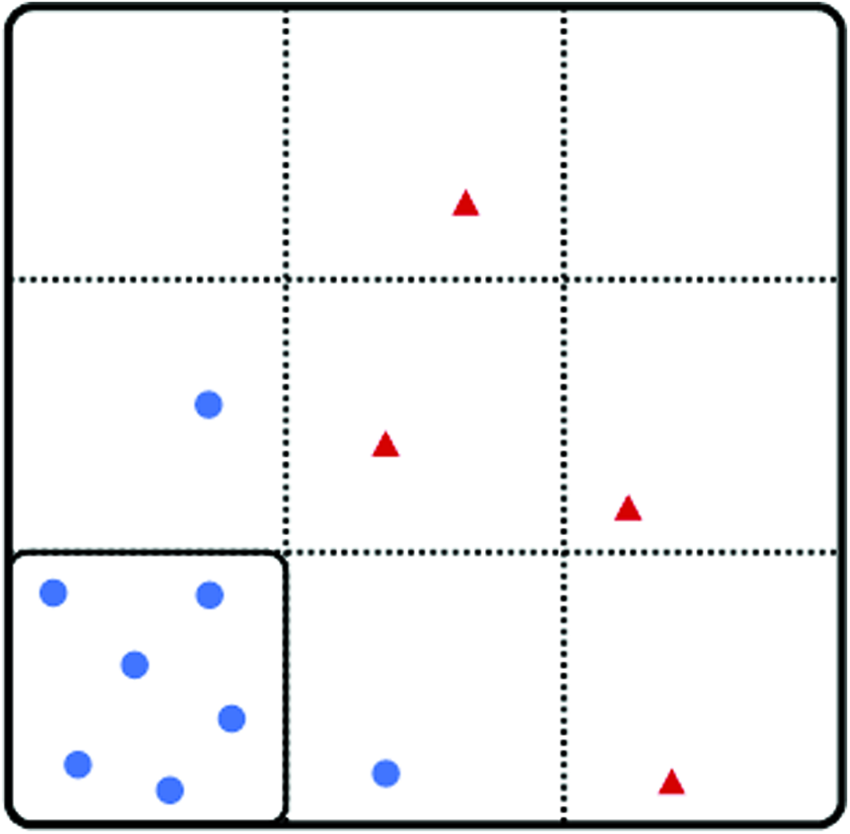
State A. Blue circles, Democratic voters; red triangles, Republican voters. Color images available online at www.liebertpub.com/elj

FIG. 2.

State B. Blue circles, Democratic voters; red triangles, Republican voters. Color images available online at www.liebertpub.com/elj

FIG. 3.

MCMC and Chen-like algorithm. Color images available online at www.liebertpub.com/elj

In the example visualized above, the map drawer has sought to avoid drawing districts-denoted by solid lines-that cross the dotted line boundaries. (These dotted lines denote any unit-census blocks, counties, etc.-that the mapmaker cannot or should not split under the relevant state law.) At the same time, each district must have equal population. As a result, many of the Democratic voters in State A are “packed” into a district made up of naturally clustered voters rather than divided into districts made up of both naturally clustered and dispersed voters. In State B, where Democrats happen to be more evenly distributed across the State, the same unbiased map drawer would be able to draw a map in which Democrats are less packed into districts with extremely heavy Democratic majorities. As a result, more Democratic votes will be “wasted” in State A than in State B. Thus, if we were to use the efficiency gap as our sole method of assessment, we would determine that map A was more gerrymandered than map B-when in reality this single metric on its own does not account for differences in population clustering. For map A: \documentclass{aastex}\usepackage{amsbsy}\usepackage{amsfonts}\usepackage{amssymb}\usepackage{bm}\usepackage{mathrsfs}\usepackage{pifont}\usepackage{stmaryrd}\usepackage{textcomp}\usepackage{portland, xspace}\usepackage{amsmath, amsxtra}\usepackage{upgreek}\pagestyle{empty}\DeclareMathSizes{10}{9}{7}{6}\begin{document} \begin{align*} EG = { \frac { { W_ { { \rm { blue } } } } - { W_ { { \rm { red } } } } } { 12 } } = { \frac { \left( { \left( { 3 + 2 } \right) - \left( { 0 + 1 } \right) } \right) } { 12 } } = 1/3 \end{align*} \end{document}

For map B: \documentclass{aastex}\usepackage{amsbsy}\usepackage{amsfonts}\usepackage{amssymb}\usepackage{bm}\usepackage{mathrsfs}\usepackage{pifont}\usepackage{stmaryrd}\usepackage{textcomp}\usepackage{portland, xspace}\usepackage{amsmath, amsxtra}\usepackage{upgreek}\pagestyle{empty}\DeclareMathSizes{10}{9}{7}{6}\begin{document} \begin{align*} EG = { \frac { { W_ { { \rm { red } } } } - { W_ { { \rm { blue } } } } } { 12 } } = { \frac { \left( { \left( { 2 + 2 } \right) - \left( { 1 + 1 } \right) } \right) } { 12 } } = 1/6 \end{align*} \end{document}

Indeed, the Wisconsin Legislature made a version of this argument in Gill v. Whitford, seeking to undermine use of the efficiency gap to assess the constitutionality of the map that the legislature drew (Reply Brief of Appellants in Gill v. Whitford 2018). And Justice Kennedy noted the problem in LULAC v. Perry. In order to create a judicially manageable standard, one that can be applied to states with differing geographies and voter distributions, courts need a means of controlling for particular geographies and voter distributions. Outlier analysis, described in the third and fourth parts, is a useful means of doing so, since it compares a given district map to a space of hypothetical, valid maps drawn for the same state (Chen and Rodden 2015).

Outlier Analysis

Outlier analysis seeks to compare a particular map to the space of reasonable, possible maps, or to some proxy for that space. If the map is an outlier compared to the space, this fact is used to support an inference of illegal, discriminatory intent. It can also be used to show that a map is sufficiently harmful to voters, whether to support a showing of individual injury for standing purposes or an ultimate constitutional violation (Gill v. Whitford 2018, Kagan, J., concurring). As explained above in our introduction, the leading precedents under the Constitution on both racial and partisan gerrymandering treat discriminatory intent as a crucial, if not required, factor. Furthermore, it is likely that evidence other than the degree of substantive unfairness of a map will remain an important part of redistricting policymaking and litigation. In this part, we briefly explain how an analogous form of outlier analysis is already well established in other areas of law, such as employment discrimination.

In Hazelwood School District v. United States (1977), the Supreme Court provided a clear endorsement of outlier analysis in the context of a “pattern or practice” discrimination case brought against a public school district by the Department of Justice, under Title VII of the Civil Rights Act, which prohibits discrimination in employment based on race, sex, and some other factors. In addition to traditional forms of evidence of intentional discrimination in some individual hiring decisions, the United States also leveraged a number of pieces of quantitative empirical evidence. The Court did not set out a clear standard of what kind of statistical evidence would be sufficient on its own to constitute a prima facie case of intentional discrimination, thereby shifting the burden to the defendants to give legitimate nondiscriminatory reasons for the disparity. However, the Court did endorse a frequentist analysis of the statistical evidence as probative and helpful. As refined in future litigation it is now accepted practice (though not common given the limited financial resources of many discrimination plaintiffs' lawyers), to model intentional discrimination in a Title VII case as follows:

First, we would assume as the null hypothesis that the employer did not discriminate, that it randomly chose from all the qualified applicants or candidates. Or we might assume that the employer took many legitimate factors into account with various weights assigned to those factors, such as experience and education and prior performance evaluations, and that some random variance was incorporated into the decision on top of those factors. Second, given these assumptions we would see how likely the actual hiring results would be. If deemed very unlikely, we reject the underlying assumptions (the null hypothesis) to conclude the employer did in fact discriminate.

In a simple example, say the average number of African Americans in the qualified labor pool is 15%. If there is no discrimination going on—our null hypothesis—sometimes the employer will hire 20% African Americans, sometimes 10%, sometimes there will be a very unusual year—an outlier year—and the employer will hire only 2%, or 60%, but usually the employer will hire around 15%. The distribution of outcomes, if we ran an experiment in which the nondiscriminating employer randomly chose over and over again, would look close to a normal distribution, or bell curve. The center of the bell curve, where the outcome appeared most frequently among our experiments, would be at 15%.

Next we would look at the percentage of African Americans actually hired by the employer. Suppose it is 8%. We would factor in the difference between 8% and the center of our curve, 15%, as well as the number of data points we have actually measured—the size of our qualified applicant pool—in order to calculate the probability that we would see a difference that large or larger just by chance. In other words, do the employer's actual hiring results demonstrate that it is an outlier when compared to the distribution of nondiscriminatory outcomes, and if so, how much of an outlier is it? We would use the bell curve to help us make this determination.

Outlier analysis has been accepted in other cases, perhaps most famously Teamsters v. United States (1977), where the Court agreed that the union had discriminated against non-whites, in part based on severe statistical disparities between the race and surnames of the employees overall and those promoted to the line driver position. When the union tried to downplay the value of statistics and outlier analysis as evidence of discrimination, the Court stated that

our cases make it unmistakably clear that statistical analyses have served and will continue to serve an important role in cases in which the existence of discrimination is a disputed issue. … We have repeatedly approved the use of statistical proof, where it reached proportions comparable to those in this case, to establish a prima facie case of racial discrimination in jury selection cases. … Statistics are equally competent in proving employment discrimination. … We caution only that statistics are not irrefutable; they come in infinite variety and, like any other kind of evidence, they may be rebutted. In short, their usefulness depends on all of the surrounding facts and circumstances. (internal quotation marks and citations removed)

Developing high-quality statistical outlier analysis for partisan gerrymandering cases is clearly a promising avenue in the legal sense for those seeking to prove unconstitutional redistricting. Not only has the Supreme Court approved of the above parallel form of outlier analysis in other areas, such as employment discrimination, it has done so even though the analysis is difficult to perform perfectly. Moreover, League of Women Voters v. Pennsylvania recently accepted outlier analysis as sufficient on its own to prove unconstitutional partisan gerrymandering, Common Cause v. Rucho (2018a) recently accepted it as a major factor in demonstrating partisan gerrymandering, and some lower federal courts have accepted it as one major factor in proving racial gerrymandering. On the other hand, there are additional challenges to modeling the space to which a district map is compared that do not exist in modeling employment decisions. In particular, a massive computational challenge exists.

Determining Intent With Outlier Analysis

To conduct outlier analysis, a given district map must be compared to a collection of alternative maps. These alternative maps should be “valid” in that they reasonably abide by nonpartisan districting criteria. Although elements of this criteria are common across states (equal-population districts and district contiguity), the list has to be tailored by region.

The various methods of generating a collection of random and “valid” maps begin with a common setup. Small geographic units need to be sorted into larger districts to form a statewide district map. It should be noted that while the smallest geographic unit for which we have demographic data is the Census block, random map generation in the literature generally takes place at a higher level of aggregation: precincts, wards, block groups, etc., are combined to form districts.

More formally, given n geographic units: \documentclass{aastex}\usepackage{amsbsy}\usepackage{amsfonts}\usepackage{amssymb}\usepackage{bm}\usepackage{mathrsfs}\usepackage{pifont}\usepackage{stmaryrd}\usepackage{textcomp}\usepackage{portland, xspace}\usepackage{amsmath, amsxtra}\usepackage{upgreek}\pagestyle{empty}\DeclareMathSizes{10}{9}{7}{6}\begin{document} \begin{align*} U = { \rm{ }} \left\{ {{U_1} , { \rm{ }}.{ \rm{ }}.{ \rm{ }}.{ \rm{ }} , {U_n}} \right\} \end{align*} \end{document}

and k districts: \documentclass{aastex}\usepackage{amsbsy}\usepackage{amsfonts}\usepackage{amssymb}\usepackage{bm}\usepackage{mathrsfs}\usepackage{pifont}\usepackage{stmaryrd}\usepackage{textcomp}\usepackage{portland, xspace}\usepackage{amsmath, amsxtra}\usepackage{upgreek}\pagestyle{empty}\DeclareMathSizes{10}{9}{7}{6}\begin{document} \begin{align*} D = { \rm{ }} \left\{ {{D_1} , { \rm{ }}.{ \rm{ }}.{ \rm{ }}.{ \rm{ }} , {D_k}} \right\} \end{align*} \end{document}

each \documentclass{aastex}\usepackage{amsbsy}\usepackage{amsfonts}\usepackage{amssymb}\usepackage{bm}\usepackage{mathrsfs}\usepackage{pifont}\usepackage{stmaryrd}\usepackage{textcomp}\usepackage{portland, xspace}\usepackage{amsmath, amsxtra}\usepackage{upgreek}\pagestyle{empty}\DeclareMathSizes{10}{9}{7}{6}\begin{document} $${U_i} , i \in \left\{ {1 , \ldots , n} \right\} $$ \end{document} needs to be assigned to one district \documentclass{aastex}\usepackage{amsbsy}\usepackage{amsfonts}\usepackage{amssymb}\usepackage{bm}\usepackage{mathrsfs}\usepackage{pifont}\usepackage{stmaryrd}\usepackage{textcomp}\usepackage{portland, xspace}\usepackage{amsmath, amsxtra}\usepackage{upgreek}\pagestyle{empty}\DeclareMathSizes{10}{9}{7}{6}\begin{document} $${D_j} , j \in \left\{ {1 , \ldots , k} \right\} $$ \end{document} . Districting criteria aside we are interested in the all the ways n units can be assigned to k districts. Each method of assigning the units constitutes a separate map.

Although the problem formulation may appear straightforward, the space of all possible maps—each element of which is a particular sorting of units into districts—is so large that it poses significant computational hurdles. As Cho and Liu (2016) point out: “Even with a modest number of units, the scale of the unconstrained map-making problem is awesome. If one wanted to divide n = 55 units into k = 6 districts, the number of possibilities is 8.7 × 10³⁹, a formidable number. There have been fewer than 10¹⁸ seconds since the beginning of the universe.”

Whittling down the space of maps to those that are “valid” by districting standards helps with the scale problem, but not enough that full enumeration of the space is possible. Generating a map ensemble for outlier analysis—i.e., a collection of maps to compare a given map to via some fairness metric—requires choosing a representative sample of maps from the space. A robust sampling method requires some kind of heuristic certification of representative sampling or another rigorous source of statistical significance. Ideally samplers won't get “stuck”-oversampling certain regions and skewing the resulting ensemble. The ability for a sampler to “jump” around the space is particularly important when considering how large patches of the map space can contain nearly identical maps. Liu et al. (2016) refer to these as “vast plateaus” in the space. Liu et al. (2016) refer to the fact that because districts are formed by combining geographic units, a unit that is near a district border in one map can be swapped into an adjacent district to form a new map. In this way, large numbers of maps that are “close” to each other in the map space can have near-identical compactness, contiguity, and county-splitting properties. A good sampler will capture maps that vary across these metrics while remaining valid by districting standards.

Next we examine how several teams of researchers traverse the map space to generate map ensembles.

Making maps from scratch

The literature shows two ways to begin random map generation to sample the map space: start with an existing map and randomly perturb district boundaries or begin anew, building districts from scratch. The second technique, explored in this section, can be ad hoc and lacks a mathematical proof that it adequately samples the map space (Common Cause v. Rucho 2018a). Furthermore, districting criteria are often incorporated in a non-rigorous fashion.

The team that has gained the most traction with this method in recent redistricting studies and litigation is Jowei Chen and Jonathan Rodden. Using their own random map algorithm they have studied the effects of human geography on partisan bias (Chen and Rodden 2013), assessed whether the 2012 Florida congressional map was a partisan gerrymander (Chen and Rodden 2015), and Chen has served as an expert witness in multiple redistricting cases (as of and including League of Women Voters v. Pennsylvania [2018], Chen had provided expert reports in 8 cases and testified at trial in 4 of them. See Chen [2017] for list of cases). Their algorithm can be summarized as follows (from Chen and Rodden's 2013 and 2015 papers): starting at the precinct level, label each precinct as its own district. Randomly select one of the districts, then choose the closest district from amongst its bordering neighbors (using a “closest centroid” definition). Combine the two districts. Now the original number of districts has been decreased by one. Repeat these initial steps until the desired number of districts are made.

The above steps address contiguity but not population equality. To incorporate this criterion, the algorithm continues: Choose the pair of districts bordering one another with the greatest population disparity. In the more populated district identify the precincts that can be transferred to the less populated district (i.e., those along the border that wouldn't violate contiguity requirements). Of these, pick the closest precinct to transfer (again using a “closest centroid”). This second set of steps is repeated until the population in each district is equal—to within a desired threshold (Chen and Rodden 2015); (Chen & Rodden 2013) (In later work Chen changes his closest centroid approach to selecting neighboring units randomly for transfer (Jowei Chen, Trial transcript in League of Women Voters vs. Pennsylvania, 2017)).

Chen and Rodden additionally claim that their algorithm preserves district compactness, as a precinct that is reassigned can only be transferred to a neighboring district. The algorithm can also consider lower priority criteria such as avoiding municipal splits when deciding whether to incorporate random units into their existing districts in a given simulation (Jowei Chen, Trial transcript in League of Women Voters vs. Pennsylvania, 2017). It should be noted that we are only able to describe Chen's algorithm in general terms because we have been unable to view his code. We have therefore gleaned details about his approach from his papers and expert witness testimony.

Cirincione et al. (2000) developed a similar map generator using Census block groups as building blocks for districts. Cirincione et al. (2000) use a combination of four algorithms, all of which begin with a randomly selected block group on which to build a map's first district. The “contiguity” algorithm randomly chooses a block group from the initial block's contiguous, unassigned neighbors (its “perimeter list”). The algorithm continues until the district is populated, then begins again with a new district. The “compactness” algorithm requires that a block chosen from the perimeter list be within the minimum bounding rectangle of the growing district. The “county integrity” algorithm picks blocks from the perimeter list that are in Census tracts already included in the developing district. The “county integrity and compactness” algorithm combines these criteria (Cirincione et al. 2000).

Neither of the above approaches includes a method for attempting to representatively sample the space of valid maps (or those that are consistent with map criteria). Fifield (2018) demonstrates this by using a Chen-like algorithm (developed in Altman and McDonald [2011]) that fails to accurately sample the map space in even the toy example of partitioning 25 precincts in Florida into three contiguous districts. Because there are so few units (25) to arrange in this example, the collection of all possible maps is fully enumerable. A fairness score can be assigned to each member of the population, resulting in a full histogram that an algorithm can try to mimic through a random subsampling of maps. The Chen-like algorithm oversamples the space in some areas and undersamples in others. Furthermore it faces these challenges with only one constraint (contiguity) and this very small number of precincts and districts.

Other researchers who have approached sampling the map space via “ground-up” map generators (i.e., not starting with an existing map) include Rossiter and Johnston (1981) and Altman and McDonald (2011).

The above algorithms, although ad hoc, use districting criteria to guide map making. They suggest it's only sensible to compare a contested district map to a collection of maps subject to the same nonpartisan guidelines (compactness, contiguity, etc.). The baseline ensemble of maps should be “likely” maps that a state legislature or districting commission could draw if following the state's mapping criteria. The next section looks at methods of sampling using a more formal notion of “likely” maps. Additionally, they are based on algorithms that are designed to sample the map space according to a probability distribution.

MCMC map sampling

The theory of MCMC sampling

Probability distributions—functions that return the probability that underlying events will occur—are sometimes difficult to draw samples from. In the context of district maps, some researchers seek to draw random samples from a distribution that labels maps according to their likelihood, or how closely they follow districting criteria Banghia (2017). For example, a map with highly compact districts and deviation from population equality of less than one percent would be more likely than a map with less compact districts and a population deviation of five percent. Other researchers have opted to sample valid maps uniformly, giving them equal weight in constructing an ensemble (Chikina, 2017; Fifield, 2018). Both methods have been tried in court with some success. If one can randomly select maps according to a distribution, we will have a collection of maps against which we can determine if an adopted state map is an outlier.

Markov Chain Monte Carlo (MCMC) methods are techniques to collect samples from distributions that are difficult to draw from directly. MCMC creates a “random walk” through the event space (in our case the map space). After the algorithm continues for long enough, or the Markov Chain “mixes,” the samples it picks will be from something nearly identical to the target distribution P(x). One difficulty with MCMC is knowing how many steps are sufficient to reach this point.

Part of MCMC's advantage is that given a distribution P(x) that lacks a closed form or is otherwise intractable, all that is required for the most common MCMC algorithm (Metropolis-Hastings) is a function z(x) that is proportional to P(x). Starting with a point in the space x₀, the algorithm proposes a candidate x' for the next step in the random walk. To decide whether or not to adopt this step the acceptance ratio is evaluated: \documentclass{aastex}\usepackage{amsbsy}\usepackage{amsfonts}\usepackage{amssymb}\usepackage{bm}\usepackage{mathrsfs}\usepackage{pifont}\usepackage{stmaryrd}\usepackage{textcomp}\usepackage{portland, xspace}\usepackage{amsmath, amsxtra}\usepackage{upgreek}\pagestyle{empty}\DeclareMathSizes{10}{9}{7}{6}\begin{document} \begin{align*} { \frac { P \left( { x ^\prime } \right) } { P \left( { { x_0 } } \right) } } = { \frac { z \left( { x ^\prime } \right) } { z \left( { { x_0 } } \right) } } \end{align*} \end{document}

(here the proposal density is assumed to be symmetric). If the ratio is greater than one then x' is more likely than x₀ according to the distribution P(x) and is therefore accepted. If the ratio is smaller than one the candidate is accepted according to a probability that depends on the ratio's value. As long as the Markov chain (or the chain of samples the algorithm chooses) is constructed properly (follows the key assumptions of the MCMC framework), the theory says that sampling will eventually be from the near identical target P(x) (Chib and Greenberg 1995).

MCMC applied to the districting problem

As an example of MCMC applied to the districting problem we look to the approach outlined in Banghia et al. (2017). The team uses MCMC sampling to randomly generate 24,000 U.S. House district maps for North Carolina (13 districts) using adopted state maps from 2012, 2016, and a judges' committee (among others) as starting points for their algorithm. They integrate state districting criteria into a map-scoring function which is then used to define a probability distribution. The distribution can weight maps that closely follow the criteria as more likely than others. This likelihood measure in turn guides the sampling process according to MCMC.

More formally, using the notation from the beginning of the section and adopting the convention used by Banghia et al. (2017), a district map is denoted: \documentclass{aastex}\usepackage{amsbsy}\usepackage{amsfonts}\usepackage{amssymb}\usepackage{bm}\usepackage{mathrsfs}\usepackage{pifont}\usepackage{stmaryrd}\usepackage{textcomp}\usepackage{portland, xspace}\usepackage{amsmath, amsxtra}\usepackage{upgreek}\pagestyle{empty}\DeclareMathSizes{10}{9}{7}{6}\begin{document} \begin{align*} \xi :U \to \left\{ {{D_1} , \ldots , {D_k}} \right\} \end{align*} \end{document}

where U is the set of geographic units to be sorted into k districts. In Banghia et al. (2017), these units are voter tabulation districts (VTDs). Voter tabulation districts are represented by vertices, and adjacent VTDs are connected by edges. With this setup, Banghia et al. (2017) defines a scoring function for each map: \documentclass{aastex}\usepackage{amsbsy}\usepackage{amsfonts}\usepackage{amssymb}\usepackage{bm}\usepackage{mathrsfs}\usepackage{pifont}\usepackage{stmaryrd}\usepackage{textcomp}\usepackage{portland, xspace}\usepackage{amsmath, amsxtra}\usepackage{upgreek}\pagestyle{empty}\DeclareMathSizes{10}{9}{7}{6}\begin{document} \begin{align*} J \left( \xi \right) = {w_p}{J_p} \left( \xi \right) + {w_I}{J_I} \left( \xi \right) + {w_c}{J_c} \left( \xi \right) + {w_m}{J_m} \left( \xi \right) \end{align*} \end{document}

where the four components of the score measure population equality between districts, compactness (via a district boundary to area ratio), county splits, and a proxy for adherence to the Voting Rights Act (VRA) (giving better scores to maps with the same number of districts with as much African American representation as the 2016 North Carolina map). The w coefficients determine the weights of each districting criteria and are computed in a calibration process. Each piece of the score is lower the better the map \documentclass{aastex}\usepackage{amsbsy}\usepackage{amsfonts}\usepackage{amssymb}\usepackage{bm}\usepackage{mathrsfs}\usepackage{pifont}\usepackage{stmaryrd}\usepackage{textcomp}\usepackage{portland, xspace}\usepackage{amsmath, amsxtra}\usepackage{upgreek}\pagestyle{empty}\DeclareMathSizes{10}{9}{7}{6}\begin{document} $$\xi$$ \end{document} follows its corresponding criteria. For example, the population score is given by: \documentclass{aastex}\usepackage{amsbsy}\usepackage{amsfonts}\usepackage{amssymb}\usepackage{bm}\usepackage{mathrsfs}\usepackage{pifont}\usepackage{stmaryrd}\usepackage{textcomp}\usepackage{portland, xspace}\usepackage{amsmath, amsxtra}\usepackage{upgreek}\pagestyle{empty}\DeclareMathSizes{10}{9}{7}{6}\begin{document} \begin{align*} { J_p } \left( \xi \right) = \sqrt { \mathop \sum \limits_ { i = 1 } ^ { 13 } { \rm { } } { { \left( { { \frac { { \rm { pop } } { D_i } \left( \xi \right) } { { \rm { po } } { { \rm { p } } _ { { \rm { ideal } } } } } } - 1 } \right) } ^2 } } \end{align*} \end{document}

where \documentclass{aastex}\usepackage{amsbsy}\usepackage{amsfonts}\usepackage{amssymb}\usepackage{bm}\usepackage{mathrsfs}\usepackage{pifont}\usepackage{stmaryrd}\usepackage{textcomp}\usepackage{portland, xspace}\usepackage{amsmath, amsxtra}\usepackage{upgreek}\pagestyle{empty}\DeclareMathSizes{10}{9}{7}{6}\begin{document} $${ \rm{pop}}{D_i} \left( \xi \right)$$ \end{document} is the population of district i in district map \documentclass{aastex}\usepackage{amsbsy}\usepackage{amsfonts}\usepackage{amssymb}\usepackage{bm}\usepackage{mathrsfs}\usepackage{pifont}\usepackage{stmaryrd}\usepackage{textcomp}\usepackage{portland, xspace}\usepackage{amsmath, amsxtra}\usepackage{upgreek}\pagestyle{empty}\DeclareMathSizes{10}{9}{7}{6}\begin{document} $$\xi$$ \end{document} and pop_ideal is the population of North Carolina divided by its 13 districts. We see that if the districts are equally populated then \documentclass{aastex}\usepackage{amsbsy}\usepackage{amsfonts}\usepackage{amssymb}\usepackage{bm}\usepackage{mathrsfs}\usepackage{pifont}\usepackage{stmaryrd}\usepackage{textcomp}\usepackage{portland, xspace}\usepackage{amsmath, amsxtra}\usepackage{upgreek}\pagestyle{empty}\DeclareMathSizes{10}{9}{7}{6}\begin{document} $${J_p} \left( \xi \right)$$ \end{document} is 0. Each subscore is similarly defined so that lower values are better. The best maps (i.e., those that most closely follow districting criteria) therefore minimize the overall score \documentclass{aastex}\usepackage{amsbsy}\usepackage{amsfonts}\usepackage{amssymb}\usepackage{bm}\usepackage{mathrsfs}\usepackage{pifont}\usepackage{stmaryrd}\usepackage{textcomp}\usepackage{portland, xspace}\usepackage{amsmath, amsxtra}\usepackage{upgreek}\pagestyle{empty}\DeclareMathSizes{10}{9}{7}{6}\begin{document} $${J_p} \left( \xi \right)$$ \end{document} .

MCMC sampling requires a probability distribution to guide “walking” through the map space. Banghia et al. (2017) chooses a distribution that treats better maps—those more closely aligned with districting criteria—as more likely to occur. The probability density function used in Banghia et al. 2017) is: \documentclass{aastex}\usepackage{amsbsy}\usepackage{amsfonts}\usepackage{amssymb}\usepackage{bm}\usepackage{mathrsfs}\usepackage{pifont}\usepackage{stmaryrd}\usepackage{textcomp}\usepackage{portland, xspace}\usepackage{amsmath, amsxtra}\usepackage{upgreek}\pagestyle{empty}\DeclareMathSizes{10}{9}{7}{6}\begin{document} \begin{align*} { P_ \beta } \left( \xi \right) = { \frac { { e^ { - \beta J \left( \xi \right) } } } { { Z_ \beta } } } \end{align*} \end{document}

where Z is a normalizing term. We can see that for fixed \documentclass{aastex}\usepackage{amsbsy}\usepackage{amsfonts}\usepackage{amssymb}\usepackage{bm}\usepackage{mathrsfs}\usepackage{pifont}\usepackage{stmaryrd}\usepackage{textcomp}\usepackage{portland, xspace}\usepackage{amsmath, amsxtra}\usepackage{upgreek}\pagestyle{empty}\DeclareMathSizes{10}{9}{7}{6}\begin{document} $$\beta$$ \end{document} , a better map (which corresponds to a lower value of \documentclass{aastex}\usepackage{amsbsy}\usepackage{amsfonts}\usepackage{amssymb}\usepackage{bm}\usepackage{mathrsfs}\usepackage{pifont}\usepackage{stmaryrd}\usepackage{textcomp}\usepackage{portland, xspace}\usepackage{amsmath, amsxtra}\usepackage{upgreek}\pagestyle{empty}\DeclareMathSizes{10}{9}{7}{6}\begin{document} $$J \left( \xi \right)$$ \end{document} ) results in a higher probability.

The next major component of the MCMC setup is a means to propose a next step in the “walk” through the map space. For this Banghia et al. (2017) randomly choose a contested edge, or an edge that connects adjacent VTDs lying in different districts in the current map \documentclass{aastex}\usepackage{amsbsy}\usepackage{amsfonts}\usepackage{amssymb}\usepackage{bm}\usepackage{mathrsfs}\usepackage{pifont}\usepackage{stmaryrd}\usepackage{textcomp}\usepackage{portland, xspace}\usepackage{amsmath, amsxtra}\usepackage{upgreek}\pagestyle{empty}\DeclareMathSizes{10}{9}{7}{6}\begin{document} $$\xi$$ \end{document} . One of the two VTDs (that are connected by this contested edge) is then randomly selected to swap out of its own district and into the neighboring one (that contains the other VTD from the pair). This new proposed map \documentclass{aastex}\usepackage{amsbsy}\usepackage{amsfonts}\usepackage{amssymb}\usepackage{bm}\usepackage{mathrsfs}\usepackage{pifont}\usepackage{stmaryrd}\usepackage{textcomp}\usepackage{portland, xspace}\usepackage{amsmath, amsxtra}\usepackage{upgreek}\pagestyle{empty}\DeclareMathSizes{10}{9}{7}{6}\begin{document} $$\xi { \rm{^\prime }}$$ \end{document} is compared to the current map \documentclass{aastex}\usepackage{amsbsy}\usepackage{amsfonts}\usepackage{amssymb}\usepackage{bm}\usepackage{mathrsfs}\usepackage{pifont}\usepackage{stmaryrd}\usepackage{textcomp}\usepackage{portland, xspace}\usepackage{amsmath, amsxtra}\usepackage{upgreek}\pagestyle{empty}\DeclareMathSizes{10}{9}{7}{6}\begin{document} $$\xi$$ \end{document} in the MCMC acceptance ratio to decide whether to adopt it as the next step in the walk through the map space.

The final piece of the sampling process is deciding when to add a map from the random walk to the map collection being used for outlier analysis. Ideally all kinds of maps that have good \documentclass{aastex}\usepackage{amsbsy}\usepackage{amsfonts}\usepackage{amssymb}\usepackage{bm}\usepackage{mathrsfs}\usepackage{pifont}\usepackage{stmaryrd}\usepackage{textcomp}\usepackage{portland, xspace}\usepackage{amsmath, amsxtra}\usepackage{upgreek}\pagestyle{empty}\DeclareMathSizes{10}{9}{7}{6}\begin{document} $$J \left( \xi \right)$$ \end{document} scores will be selected, even though they might be very far away from each other in the map-space. This means sampling needs to be able to “jump” throughout the space instead of getting stuck in only one area of maps that are likely according to \documentclass{aastex}\usepackage{amsbsy}\usepackage{amsfonts}\usepackage{amssymb}\usepackage{bm}\usepackage{mathrsfs}\usepackage{pifont}\usepackage{stmaryrd}\usepackage{textcomp}\usepackage{portland, xspace}\usepackage{amsmath, amsxtra}\usepackage{upgreek}\pagestyle{empty}\DeclareMathSizes{10}{9}{7}{6}\begin{document} $${P_ \beta } \left( \xi \right)$$ \end{document} .

To move more flexibly through the space Banghia et al. (2017) uses a process called simulated annealing which alters the value of \documentclass{aastex}\usepackage{amsbsy}\usepackage{amsfonts}\usepackage{amssymb}\usepackage{bm}\usepackage{mathrsfs}\usepackage{pifont}\usepackage{stmaryrd}\usepackage{textcomp}\usepackage{portland, xspace}\usepackage{amsmath, amsxtra}\usepackage{upgreek}\pagestyle{empty}\DeclareMathSizes{10}{9}{7}{6}\begin{document} $$\beta$$ \end{document} during sampling. Note that for low values of \documentclass{aastex}\usepackage{amsbsy}\usepackage{amsfonts}\usepackage{amssymb}\usepackage{bm}\usepackage{mathrsfs}\usepackage{pifont}\usepackage{stmaryrd}\usepackage{textcomp}\usepackage{portland, xspace}\usepackage{amsmath, amsxtra}\usepackage{upgreek}\pagestyle{empty}\DeclareMathSizes{10}{9}{7}{6}\begin{document} $$\beta$$ \end{document} (consider \documentclass{aastex}\usepackage{amsbsy}\usepackage{amsfonts}\usepackage{amssymb}\usepackage{bm}\usepackage{mathrsfs}\usepackage{pifont}\usepackage{stmaryrd}\usepackage{textcomp}\usepackage{portland, xspace}\usepackage{amsmath, amsxtra}\usepackage{upgreek}\pagestyle{empty}\DeclareMathSizes{10}{9}{7}{6}\begin{document} $$\beta = 0$$ \end{document} as the extreme), each map \documentclass{aastex}\usepackage{amsbsy}\usepackage{amsfonts}\usepackage{amssymb}\usepackage{bm}\usepackage{mathrsfs}\usepackage{pifont}\usepackage{stmaryrd}\usepackage{textcomp}\usepackage{portland, xspace}\usepackage{amsmath, amsxtra}\usepackage{upgreek}\pagestyle{empty}\DeclareMathSizes{10}{9}{7}{6}\begin{document} $$\xi$$ \end{document} is closer in probability to other maps in \documentclass{aastex}\usepackage{amsbsy}\usepackage{amsfonts}\usepackage{amssymb}\usepackage{bm}\usepackage{mathrsfs}\usepackage{pifont}\usepackage{stmaryrd}\usepackage{textcomp}\usepackage{portland, xspace}\usepackage{amsmath, amsxtra}\usepackage{upgreek}\pagestyle{empty}\DeclareMathSizes{10}{9}{7}{6}\begin{document} $${P_ \beta } \left( \xi \right)$$ \end{document} . In this case the algorithm frequently accepts the proposed next steps in the random walk, and therefore the sampler moves freely about the space. When \documentclass{aastex}\usepackage{amsbsy}\usepackage{amsfonts}\usepackage{amssymb}\usepackage{bm}\usepackage{mathrsfs}\usepackage{pifont}\usepackage{stmaryrd}\usepackage{textcomp}\usepackage{portland, xspace}\usepackage{amsmath, amsxtra}\usepackage{upgreek}\pagestyle{empty}\DeclareMathSizes{10}{9}{7}{6}\begin{document} $$\beta$$ \end{document} is increased to 1, the distribution narrows around maps with better scores. In this way, the sampler can end up in different pockets of the space that each produce good, but different, maps. After studying the best treatment of \documentclass{aastex}\usepackage{amsbsy}\usepackage{amsfonts}\usepackage{amssymb}\usepackage{bm}\usepackage{mathrsfs}\usepackage{pifont}\usepackage{stmaryrd}\usepackage{textcomp}\usepackage{portland, xspace}\usepackage{amsmath, amsxtra}\usepackage{upgreek}\pagestyle{empty}\DeclareMathSizes{10}{9}{7}{6}\begin{document} $$\beta$$ \end{document} , Banghia et al. (2017) uses \documentclass{aastex}\usepackage{amsbsy}\usepackage{amsfonts}\usepackage{amssymb}\usepackage{bm}\usepackage{mathrsfs}\usepackage{pifont}\usepackage{stmaryrd}\usepackage{textcomp}\usepackage{portland, xspace}\usepackage{amsmath, amsxtra}\usepackage{upgreek}\pagestyle{empty}\DeclareMathSizes{10}{9}{7}{6}\begin{document} $$\beta = 0$$ \end{document} for 40,000 random-walk steps, increases \documentclass{aastex}\usepackage{amsbsy}\usepackage{amsfonts}\usepackage{amssymb}\usepackage{bm}\usepackage{mathrsfs}\usepackage{pifont}\usepackage{stmaryrd}\usepackage{textcomp}\usepackage{portland, xspace}\usepackage{amsmath, amsxtra}\usepackage{upgreek}\pagestyle{empty}\DeclareMathSizes{10}{9}{7}{6}\begin{document} $$\beta$$ \end{document} to 1 over 60,000 steps and leaves \documentclass{aastex}\usepackage{amsbsy}\usepackage{amsfonts}\usepackage{amssymb}\usepackage{bm}\usepackage{mathrsfs}\usepackage{pifont}\usepackage{stmaryrd}\usepackage{textcomp}\usepackage{portland, xspace}\usepackage{amsmath, amsxtra}\usepackage{upgreek}\pagestyle{empty}\DeclareMathSizes{10}{9}{7}{6}\begin{document} $$\beta$$ \end{document} at 1 for 20,000 before taking a sample. This process is repeated for each of the samples that make up the final map ensemble.

Although Banghia et al. (2017) cites several drawbacks to this approach (results can change based on the number of steps before drawing a sample, mixing time—or the time it takes to reach the target distribution—is unclear, and changing \documentclass{aastex}\usepackage{amsbsy}\usepackage{amsfonts}\usepackage{amssymb}\usepackage{bm}\usepackage{mathrsfs}\usepackage{pifont}\usepackage{stmaryrd}\usepackage{textcomp}\usepackage{portland, xspace}\usepackage{amsmath, amsxtra}\usepackage{upgreek}\pagestyle{empty}\DeclareMathSizes{10}{9}{7}{6}\begin{document} $$\beta$$ \end{document} means changing the target distribution etc.), they demonstrate a method that gets a diverse sample of maps that are deemed likely according to districting criteria. This technique was relied upon heavily by the court in Common Cause v. Rucho (2018b), on remand after Gill v. Whitford, to conclude that North Carolina's district map was unconstitutionally gerrymandered.

It should be noted that Banghia et al. (2017) devotes sections in their paper to both determining the weights in their scoring function (w_p, w_I, w_c, w_m in \documentclass{aastex}\usepackage{amsbsy}\usepackage{amsfonts}\usepackage{amssymb}\usepackage{bm}\usepackage{mathrsfs}\usepackage{pifont}\usepackage{stmaryrd}\usepackage{textcomp}\usepackage{portland, xspace}\usepackage{amsmath, amsxtra}\usepackage{upgreek}\pagestyle{empty}\DeclareMathSizes{10}{9}{7}{6}\begin{document} $$J \left( \xi \right)$$ \end{document} ) and performing a sensitivity analysis on the weight values. In practical terms, changing weights means changing the relative importance of districting criteria when randomly choosing valid maps. For example, in the extreme scenario of setting w_I to 1 and all other weights to 0, the resulting map ensemble would be dominated by those that split the fewest counties (they could violate the other districting criteria). A contested map could then only be deemed an outlier on this metric. The analysis would offer no indication of whether the contested map had to sacrifice some county cohesion to satisfy other criteria such as maintaining majority-minority districts. Although this example is extreme, it demonstrates the impact of weighting decisions in scoring functions. Banghia et al. (2017) found that changing their weights did not significantly impact results. However, deciding on reasonable ranges for weight values, and therefore reasonable variations in map ensembles, remains subject to interpretation.

Other researchers using MCMC to sample maps are Fifield et al. (2018) and Chikina et al. (2017). The approach outlined in Fifield (2018) shares a number of similarities with the MCMC process in Banghia (2017), but its differences include allowing groups of units to be transferred between districts at a time as well as re-weighting their samples to be from a uniform distribution on valid districting maps. The approach in Chikina (2017) is markedly different. Instead of aiming to sample from a close approximation of a target distribution, the team devises a method to show that a given legislative map is unlikely to be drawn from a uniform distribution (a distribution that weights valid maps equally, as opposed to the distribution used in Banghia [2017] that weights maps more closely aligned with districting criteria as being more likely) of valid districting maps. Furthermore the method does not even require that the sample be representative of the search space. Teams that have released open source MCMC code include Fifield et al (‘redist’ 2018) and most recently the Metric Geometry and Gerrymandering Group (GerryChain 2018).

Evolutionary algorithms for map construction

A third way to construct map ensembles uses evolutionary algorithms (EA), or algorithms that mimic a population's shifting and mutating over time to produce more “fit” members. In the map context, a population is a collection of district maps, and “fitness” is measured by an objective function that scores a map's features such as compactness, population equality, etc. It should be noted that although the approach below offers a different way of thinking about the map generation set up, the steps to construct new maps and “jump” through the map space are very similar to those described in the MCMC approach.

Cho, Liu, and Wang encode a district map in a “chromosome” structure: a number, or index, is assigned to each geographical unit (they use VTDs in their analysis) which is unchanged (Liu et al. 2016). Each unit then holds the value of the district to which it is assigned in a particular map (the “allele”). Each unit can be assigned to only one district. In this way, a district map can be represented as a “chromosome,” or a string of pairs of values: one indicating the unit and the other the district it's assigned to (Liu et al. 2016; Rudolph 1994).

An EA begins with an initial population, or the group from which to breed new members. The initial population in Liu et al. (2016) consists of 200 maps which are generated in one of two ways: seed units are randomly chosen across the map and built up to make the target number of districts, or seed units are chosen only along the boundary of the map with districts being built inwards. Either way each of the initial 200 maps has the correct number of contiguous districts.

To generate new members of the population, Liu et al. (2016) use a combination of mutation and crossover algorithms. Both are analogous to their evolutionary counterparts. Mutation algorithms perturb a member of the population in a randomized way (on the chromosome level, this means randomly changing a value or values in the string, or the districts to which a randomly chosen subset of VTDs are assigned). Liu et al.'s (2016) mutation algorithm chooses a sequence of districts at random. For each, a neighboring district is chosen to which a cluster of units from the original will be transferred. In this way, clumps of units are transferred from one district to another in each iteration of the mutation algorithm, with built-in constraints on population deviation across districts. This is nearly identical to how districts are swapped in the MCMC methods.

The crossover algorithm takes two members of the population and crosses them to construct a “child” map. Units that belonged to different districts in their parent maps are sorted into the correct number of contiguous districts in the child map. It is not always the case that the new map is better than the old ones (as measured by a fitness function) (Liu et al. 2016). Both crossover and mutation algorithms can make large “jumps” through the map space, producing new maps that can be significantly different than the parents (crossover) or old single map (mutation). Recall that in Banghia et al. (2017), the tool to make large jumps in the map space was changing the parameter \documentclass{aastex}\usepackage{amsbsy}\usepackage{amsfonts}\usepackage{amssymb}\usepackage{bm}\usepackage{mathrsfs}\usepackage{pifont}\usepackage{stmaryrd}\usepackage{textcomp}\usepackage{portland, xspace}\usepackage{amsmath, amsxtra}\usepackage{upgreek}\pagestyle{empty}\DeclareMathSizes{10}{9}{7}{6}\begin{document} $$\beta$$ \end{document} in the probability distribution that governed the random walk through the space. Both approaches incorporate the need to not get “stuck” sampling from a small area, ensuring the resulting map ensemble contains a wide variety of maps that follow districting criteria.

Mutation and crossover make new maps, but a score for the map is needed to decide if it should be added to the population. Maps are evaluated with a fitness score. This comes from an optimization function that can be tailored to include relevant districting criteria (compactness, competitiveness, etc.). How one weights the objectives in this function is flexible. New maps can also be subject to constraints (i.e., any map that doesn't meet a population deviation threshold across districts can be thrown out). In this way, districting criteria can be incorporated flexibly: as constraints, which apply to all maps in the population, or in the optimization function, which will rate maps that perform better as being more “fit.” Maps with bad scores are replaced with more fit maps as the EA continues and the population evolves to form a final ensemble used for outlier analysis (Liu et al. 2016).

While EAs are generally used to find a single optimal solution (in this case an optimal district map), Liu et al.'s (2016) algorithm is meant to make a population that at least exceeds some “goodness thresholds” and therefore makes a reasonable baseline set for outlier analysis (in the Maryland analysis in Cho and Liu [2016] these are derived from nonpartisan measures from the adopted district plan). Drawbacks to the approach include the required computing power. However, Cho is working with a supercomputing specialist (Yan Liu) to optimize parallelizing her approach, making her sampling much faster than that used in MCMC.

Other evolutionary algorithms for redistricting and geographic problems are described in Xiao (2008) and Galinier and Hao (1999).

Although the above methods for random map generation are very different, in order to know which performs better (i.e., does a better job at representatively sampling the space of all possible maps), we need some way to compare their outcomes. Because in almost all cases the map space isn't fully enumerable, testing different algorithms on a small test example can give an initial indication of skewedness in sampling. Fifield et al. demonstrate this approach in Fifield (2018). They constructed the graphic below.

Fifield et al. used data from a toy problem—partitioning Florida's 25 precincts in three districts with only a contiguity constraint—and assigned each map a partisan metric score (Republican Dissimilarity Index). The distribution of those scores is pictured in solid grey (how many times each score occurred in the map collection). Note that in this toy case, the map space is fully enumerable, and therefore the solid grey plot is the “right answer.” Allowing an algorithm to randomly sample the map space and plotting the frequency of the resulting map metrics can offer a comparison to the underlying fully enumerated distribution. If an algorithm perfectly sampled the space, it would match the underlying grey true distribution. The solid and dashed lines closely overlaying Fifield's figure are the results of two variations of their MCMC algorithm, which fit the distribution quite well. The less-well-fitting dashed line is a Chen/Cirincione-type algorithm (Altman & McDonald, 2011), which does not capture the map distribution. Clearly, MCMC does a better job at approximating the map-distribution than the Chen-like algorithm in this case.

It is important to note that this is not a decisive method to choose a “best” algorithm. Among other reasons it gives no indication about an algorithm's potential failure when scaled up to massive map-spaces, even if it performs well on these smaller sets. Publication of the underlying code behind additional algorithms would help facilitate these assessments, especially so that one could standardize map metric, sampling size, and additional features to draw direct comparisons.

Future Directions

While districting criteria such as contiguity, population equality, and even compactness have clear measures that can be used in map scoring and optimization functions, compliance with the VRA is less straightforward. The Act forbids maps in which voters of one racial group have “less opportunity than other members of the electorate to participate in the political process and to elect representatives of their choice.” On the other hand, the Constitution forbids racial gerrymanders, including those whose intent is to benefit historically discriminated against racial groups (Shaw v. Reno 1993). Thus, a map in a state with racially polarized voting that either packs or cracks the minority voters too excessively may violate the Voting Rights Act. However, a map that tries too strenuously to avoid this situation may violate the Constitution. In order to convince lawmakers and courts that a contested map is gerrymandered using outlier analysis, it must be compared to an ensemble of maps that comply with the VRA in a reasonable way. Therefore standards must be agreed upon for how to encode it and score its implementation in a district map. There is no such consensus yet in the literature.

Several approaches have been taken to this problem. Chen and Rodden (2015) freeze districts from the contested map that the state claims (Florida in this case) have been constructed specially for the VRA. Their simulations change districts around them. To generate a map ensemble for North Carolina, Banghia et al. (2017) refer to a former state map that was accepted by the courts for guidance. They take the percentage of African Americans in the districts designed to comply with the VRA as a baseline. In their scoring function they penalize maps that don't have the same number of districts with at least as high a percentage of African Americans. Duchin (2018) uses an MCMC approach in which she labels communities of interest as “geoclusters” and gives the option for the algorithm to require that they be kept intact or favor maps that do so. One advantage of this approach is that it doesn't adhere rigidly to how an existing map complies with the VRA, but instead allows the borders of districts to vary around the core communities. Concerns with approaches that rely on existing maps for how to comply with the VRA include the fact that these maps may overpack, and therefore dilute African American votes. Because the balance between constructing majority-minority districts and overpacking minority votes is delicate, simply deferring to a past approach that hasn't been overturned by the courts as the standard may prove inflexible in this balancing act. Additionally, in Abbott v. Perez (2018), a recent case involving both racial gerrymandering and VRA compliance, the majority and dissenting opinions, while disagreeing on the facts in the case at hand, agreed that creating opportunity districts for some voters, particularly those lacking a Section 2 right to such a district, cannot justify failure to create an opportunity district for voters who themselves possess a Section 2 right. This strongly implies that simply maintaining an opportunity district that was previously approved by a court is not sufficient for VRA compliance, where shifting evidence of block voting may have created the need for additional opportunity districts, or at least ones with different borders. The question of how to standardize scoring VRA compliance thus remains open.

On the theoretical side, gaining understanding of the space of all districting maps can offer insight into how best to traverse it in sampling. In particular, understanding how weeding out large collections of maps (due to noncontiguous districts, etc.) “breaks” the space and how or if this causes sampling to get stuck is important in interpreting resulting ensembles (for example, knowing if they're skewed in a particular fashion). Furthermore, as noted in the fourth part, more analysis is needed on how sensitive map ensembles are to changes in distributions (for MCMC sampling) or optimization functions (for EA sampling). Specifically, understanding how weighting criteria in scoring functions skews resulting ensembles is important to head off claims that map collections are too variable for reliable outlier analysis.

While many advocates of gerrymandering reform were disappointed by the Court's decision in Gill v. Whitford (2018), the efforts to firm up a standard with which to evaluate gerrymandering are still worthwhile. As the Pennsylvania State Supreme Court demonstrated in League of Women Voters v. Pennsylvania (2018), local and state courts may have the freedom to start crafting their own workable standards in redistricting cases. This could be an avenue for outlier analysis to gain popularity if there is not an overt nod towards it in future litigation before the Supreme Court. Additionally, Justice Kagan's concurring opinion in Gill v. Whitford (2018) and the district court's post-Whitford decision in Common Cause v. Rucho (2018b) support the use of outlier analysis as a way for plaintiffs to prove vote dilution in their district. Random map generation could also still be appropriate if plaintiffs decided to pursue a statewide “associational” harm, also discussed in the concurrence. In this case, alternative maps might be rated on statewide metrics, as opposed to individual district metrics when showing individual harm.

In any event, popularizing substantive fairness measures and outlier analysis, as well as publicizing their benefits and drawbacks, could be useful for independent redistricting commissions who want to compare proposed maps within a state along fairness metrics. Substantive measures can also play a role as supporting, if not sufficient, evidence to prove unconstitutional gerrymandering (Common Cause v. Rucho 2018). It is also crucial for normalizing reliable and rigorous techniques for the public to point to partisan excess in map drawing. Having a community of mathematicians, political scientists, and lawyers continue to work towards this standard will help make tools available to construct fair maps and also call out legislatures' maps that do not pass muster, with or without the courts.