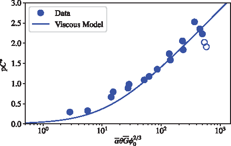
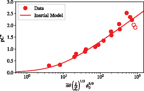
A widely applicable hydraulic flocculator design model would facilitate increased adoption of this sustainable technology. To this end, the authors previously proposed rate equations for the removal of nonsettleable aggregates in hydraulic flocculators (Pennock et al.). This work continues the prior effort by developing two models for coupled flocculation/sedimentation performance. The first model describes settled effluent turbidity for flocculators where the relative velocities between particles are dominated by viscous forces (e.g., laminar flows). Similarly, the second model applies where inertial forces dominate. Predictions of these models were compared with laboratory-scale flocculation/sedimentation data obtained from both a laminar- and a turbulent-flow flocculator. The viscous equation fit data from the laminar flow flocculator well. For the turbulent flocculator, both models gave good fits of the data, but the inertial model performed slightly better. The similarity of the two models under the experimental constraints explains this result, and further study in different conditions is needed to delineate the applicability of the models in turbulent flocculation. Given the similarity between the models and that the product of the mean fluid velocity gradient applicable to laminar flow \documentclass{aastex}\usepackage{amsbsy}\usepackage{amsfonts}\usepackage{amssymb}\usepackage{bm}\usepackage{mathrsfs}\usepackage{pifont}\usepackage{stmaryrd}\usepackage{textcomp}\usepackage{portland, xspace}\usepackage{amsmath, amsxtra}\usepackage{upgreek}\pagestyle{empty}\DeclareMathSizes{10}{9}{7}{6}\begin{document}
$$( \overline G )$$
\end{document} and hydraulic residence time \documentclass{aastex}\usepackage{amsbsy}\usepackage{amsfonts}\usepackage{amssymb}\usepackage{bm}\usepackage{mathrsfs}\usepackage{pifont}\usepackage{stmaryrd}\usepackage{textcomp}\usepackage{portland, xspace}\usepackage{amsmath, amsxtra}\usepackage{upgreek}\pagestyle{empty}\DeclareMathSizes{10}{9}{7}{6}\begin{document}
$$( \theta )$$
\end{document}, \documentclass{aastex}\usepackage{amsbsy}\usepackage{amsfonts}\usepackage{amssymb}\usepackage{bm}\usepackage{mathrsfs}\usepackage{pifont}\usepackage{stmaryrd}\usepackage{textcomp}\usepackage{portland, xspace}\usepackage{amsmath, amsxtra}\usepackage{upgreek}\pagestyle{empty}\DeclareMathSizes{10}{9}{7}{6}\begin{document}
$$\overline G \theta$$
\end{document}, has historically been used in flocculator design, it is recommended that the viscous flocculation model introduced in this article be used. The new flocculation models have a single adjustable parameter and, in addition to being able to predict settled effluent turbidity from coagulant dose, also provide reasonable estimates of flocculator design parameters from first principles and dimensional analysis.
Introduction
Hydraulic flocculators have significant advantages over mechanically mixed flocculators. They have no moving parts, resulting in lower operation (electricity) and maintenance (repair and replacement) costs. In addition, hydraulic flocculators approach plug flow, which improves reaction kinetics because the inflow is not diluted. They are also far less vulnerable to short-circuiting compared with mechanically mixed flocculators, which operationally approach continuous-flow stirred tank reactors (Benjamin and Lawler, 2013). Hydraulic flocculators have been chosen for their sustainability in drinking water treatment plants, such as the gravity-powered plants designed by Cornell University's AguaClara program implemented in Honduras, as well as those in South Africa studied by Haarhoff (1998).
Flocculation changes the particle size distribution (PSD) received by the downstream water treatment processes of sedimentation and filtration. Improving drinking water treatment plant performance, therefore, requires the optimization of flocculation to give the best PSD for subsequent processes. To optimize flocculation performance, it is useful to develop a generalized, mechanistically based flocculation model to guide design and operation of flocculators.
Haarhoff (1998) developed an empirical design approach for horizontal baffled hydraulic flocculators, and then verified these guidelines with computational fluid dynamics (CFD) simulations (Haarhoff and van der Walt, 2001). Although this work is an excellent resource, their design guidance is limited to one geometry and it does not provide performance predictions.
Several researchers have developed population balance models (PBM), which are sets of differential equations applied to a control volume defined by the entire flocculator (i.e., Eulerian frame of reference) based on the model proposed by Smoluchowski (1917). These are numerically integrated to solve for the PSD over time. An example of this approach applied to mechanically mixed flocculators is given in Ducoste (2002). This approach has the advantage of being theoretically based and providing predictions for the evolution of PSD through the process. Challenges in applying this approach include finding sufficiently accurate estimates of the initial conditions, the hydraulic conditions within the flocculator, and the values of attachment efficiencies that are unknown functions of the coagulant dose and raw water quality. In addition, especially when CFD simulations are used to model the hydraulic conditions, this approach suffers the disadvantage of being computationally intensive, which may be too cumbersome for design and operation (Prat and Ducoste, 2007; Bridgeman et al., 2010).
Argaman and Kaufman (1970) proposed an analytical solution to Smoluchowski's (1917) PBM by making a number of simplifying assumptions and integrating, creating a flocculator performance prediction equation that can be used for design and operation of both plug flow (hydraulic) and completely mixed (mechanical) flocculators. Liu et al. (2004) refined this formulation to enhance predictions for hydraulic flocculators that have nonuniform hydraulic conditions. The Argaman-Kaufman equation has three experimentally derived constants. Two are physically based, representing the rates of aggregation and breakup in the process, and each can be derived from a different set of experiments, each containing at least nine runs (Haarhoff and Joubert, 1997). The third constant has no physical meaning, and is unique to each flocculator (Liu et al., 2004). Determining the values of these parameters presents an obstacle to using the Argaman-Kaufman model to design new flocculators.
This work aims to further simplify hydraulic flocculator performance prediction by integrating from an alternative differential equation to the Smoluchowski equation that Argaman and Kaufman (1970) integrated. This differential equation, a Lagrangian model proposed by Pennock et al. (2016), achieves simplicity by modeling the journey of a characteristic nonsettleable particle through the flocculator. It is reasonable to track nonsettleable particles to the exclusion of flocs that have grown large enough to be settleable, because the nonsettleable, or residual, particles determine flocculation performance. In addition, the majority of successful collisions involving nonsettleable particles appear to be collisions with other nonsettleable particles. This hypothesis is suggested by Casson and Lawler (1990) who found in flocculating a trimodal distribution of particles that homocoagulation dominated. They cited Adler (1981), who found that numerical simulations accounting for the effects of hydrodynamic, van der Waals, and double-layer forces generally gave higher collision efficiencies for particles of similar size. It is therefore assumed that the rate of nonsettleable particles' conversion to settleable flocs can be modeled as a function of the concentration of nonsettleable particles.
In their article, Pennock et al. (2016) began with a first-order model, which relates the rate of successful collisions between nonsettleable particles to the time between collisions:
\documentclass{aastex}\usepackage{amsbsy}\usepackage{amsfonts}\usepackage{amssymb}\usepackage{bm}\usepackage{mathrsfs}\usepackage{pifont}\usepackage{stmaryrd}\usepackage{textcomp}\usepackage{portland, xspace}\usepackage{amsmath, amsxtra}\usepackage{upgreek}\pagestyle{empty}\DeclareMathSizes{10}{9}{7}{6}\begin{document}
\begin{align*}
{ \frac { { \rm d } { N_ { \rm c } } } { { \rm d } t } } = { \frac { { \rm { \overline \Gamma } } } { \overline { { t_ { \rm c } } } } } , \tag { 1 }
\end{align*}
\end{document}
where Nc is the number of successful collisions between nonsettleable particles, \documentclass{aastex}\usepackage{amsbsy}\usepackage{amsfonts}\usepackage{amssymb}\usepackage{bm}\usepackage{mathrsfs}\usepackage{pifont}\usepackage{stmaryrd}\usepackage{textcomp}\usepackage{portland, xspace}\usepackage{amsmath, amsxtra}\usepackage{upgreek}\pagestyle{empty}\DeclareMathSizes{10}{9}{7}{6}\begin{document}
$$ { \frac { { \rm d } { N_ { \rm c } } } { { \rm d } t } } $$
\end{document} is the rate at which these collisions occur, \documentclass{aastex}\usepackage{amsbsy}\usepackage{amsfonts}\usepackage{amssymb}\usepackage{bm}\usepackage{mathrsfs}\usepackage{pifont}\usepackage{stmaryrd}\usepackage{textcomp}\usepackage{portland, xspace}\usepackage{amsmath, amsxtra}\usepackage{upgreek}\pagestyle{empty}\DeclareMathSizes{10}{9}{7}{6}\begin{document}
$${ \rm{ \overline \Gamma }}$$
\end{document} is the mean fractional coverage of particle surface area by coagulant precipitates, and \documentclass{aastex}\usepackage{amsbsy}\usepackage{amsfonts}\usepackage{amssymb}\usepackage{bm}\usepackage{mathrsfs}\usepackage{pifont}\usepackage{stmaryrd}\usepackage{textcomp}\usepackage{portland, xspace}\usepackage{amsmath, amsxtra}\usepackage{upgreek}\pagestyle{empty}\DeclareMathSizes{10}{9}{7}{6}\begin{document}
$$\overline {{t_{ \rm{c}}}}$$
\end{document} is the mean time between collisions of nonsettleable particles. The mean fractional coverage, \documentclass{aastex}\usepackage{amsbsy}\usepackage{amsfonts}\usepackage{amssymb}\usepackage{bm}\usepackage{mathrsfs}\usepackage{pifont}\usepackage{stmaryrd}\usepackage{textcomp}\usepackage{portland, xspace}\usepackage{amsmath, amsxtra}\usepackage{upgreek}\pagestyle{empty}\DeclareMathSizes{10}{9}{7}{6}\begin{document}
$${ \rm{ \overline \Gamma }}$$
\end{document}, is akin to the attachment efficiency term in other flocculation models (e.g., Casson and Lawler, 1990; Ducoste, 2002) and has a physical basis, given knowledge of the concentrations and diameters of colloidal particles and of coagulant precipitate clusters (Swetland et al., 2014). The inclusion of \documentclass{aastex}\usepackage{amsbsy}\usepackage{amsfonts}\usepackage{amssymb}\usepackage{bm}\usepackage{mathrsfs}\usepackage{pifont}\usepackage{stmaryrd}\usepackage{textcomp}\usepackage{portland, xspace}\usepackage{amsmath, amsxtra}\usepackage{upgreek}\pagestyle{empty}\DeclareMathSizes{10}{9}{7}{6}\begin{document}
$${ \rm{ \overline \Gamma }}$$
\end{document} in Equation (1) converts the general collisions described by \documentclass{aastex}\usepackage{amsbsy}\usepackage{amsfonts}\usepackage{amssymb}\usepackage{bm}\usepackage{mathrsfs}\usepackage{pifont}\usepackage{stmaryrd}\usepackage{textcomp}\usepackage{portland, xspace}\usepackage{amsmath, amsxtra}\usepackage{upgreek}\pagestyle{empty}\DeclareMathSizes{10}{9}{7}{6}\begin{document}
$$\overline {{t_{ \rm{c}}}}$$
\end{document} to the successful collisions described by \documentclass{aastex}\usepackage{amsbsy}\usepackage{amsfonts}\usepackage{amssymb}\usepackage{bm}\usepackage{mathrsfs}\usepackage{pifont}\usepackage{stmaryrd}\usepackage{textcomp}\usepackage{portland, xspace}\usepackage{amsmath, amsxtra}\usepackage{upgreek}\pagestyle{empty}\DeclareMathSizes{10}{9}{7}{6}\begin{document}
${{\rm d}{N_{\rm c}} \over {{\rm d}t}}$
\end{document}. The concept behind \documentclass{aastex}\usepackage{amsbsy}\usepackage{amsfonts}\usepackage{amssymb}\usepackage{bm}\usepackage{mathrsfs}\usepackage{pifont}\usepackage{stmaryrd}\usepackage{textcomp}\usepackage{portland, xspace}\usepackage{amsmath, amsxtra}\usepackage{upgreek}\pagestyle{empty}\DeclareMathSizes{10}{9}{7}{6}\begin{document}
$${ \rm{ \overline \Gamma }}$$
\end{document} differs from random sequential adsorption (RSA) in that it allows for the possibility of coagulant precipitate clusters stacking on top of previously attached coagulant precipitate clusters, thereby approaching complete coverage asymptotically (Feder, 1980; Swetland et al., 2014). The calculation of \documentclass{aastex}\usepackage{amsbsy}\usepackage{amsfonts}\usepackage{amssymb}\usepackage{bm}\usepackage{mathrsfs}\usepackage{pifont}\usepackage{stmaryrd}\usepackage{textcomp}\usepackage{portland, xspace}\usepackage{amsmath, amsxtra}\usepackage{upgreek}\pagestyle{empty}\DeclareMathSizes{10}{9}{7}{6}\begin{document}
$${ \rm{ \overline \Gamma }}$$
\end{document} also accounts for the loss of coagulant to reactor walls, with the assumption that the coagulant has equal affinity for particle and wall surfaces (Swetland et al., 2014).
The probability that two nonsettleable particles attach is expected to be equal to the probability that at least one of the colliding particles has a precipitated coagulant nanoparticle at the initial contact point. The original use of \documentclass{aastex}\usepackage{amsbsy}\usepackage{amsfonts}\usepackage{amssymb}\usepackage{bm}\usepackage{mathrsfs}\usepackage{pifont}\usepackage{stmaryrd}\usepackage{textcomp}\usepackage{portland, xspace}\usepackage{amsmath, amsxtra}\usepackage{upgreek}\pagestyle{empty}\DeclareMathSizes{10}{9}{7}{6}\begin{document}
$${ \rm{ \overline \Gamma }}$$
\end{document} by Pennock et al. (2016) to describe the fraction of collisions that are successful did not properly account for this probability of a successful collision. While \documentclass{aastex}\usepackage{amsbsy}\usepackage{amsfonts}\usepackage{amssymb}\usepackage{bm}\usepackage{mathrsfs}\usepackage{pifont}\usepackage{stmaryrd}\usepackage{textcomp}\usepackage{portland, xspace}\usepackage{amsmath, amsxtra}\usepackage{upgreek}\pagestyle{empty}\DeclareMathSizes{10}{9}{7}{6}\begin{document}
$${ \rm{ \overline \Gamma }}$$
\end{document} is the probability of a single nonsettleable particle surface colliding at a site on its surface that is covered with a coagulant precipitate, the collision involves two particles, and so the probability of success is higher.
It is simplest to derive the probability of attachment from the probability that neither particle has a coagulant precipitate at the point where the two particles collide, since the probability of a successful collision includes the probabilities of one particle and of both particles having a coagulant precipitate. The probability of one particle colliding at a point without a coagulant precipitate is \documentclass{aastex}\usepackage{amsbsy}\usepackage{amsfonts}\usepackage{amssymb}\usepackage{bm}\usepackage{mathrsfs}\usepackage{pifont}\usepackage{stmaryrd}\usepackage{textcomp}\usepackage{portland, xspace}\usepackage{amsmath, amsxtra}\usepackage{upgreek}\pagestyle{empty}\DeclareMathSizes{10}{9}{7}{6}\begin{document}
$$\left( {1 - { \rm{ \overline \Gamma }}} \right)$$
\end{document}, so the probability of neither particle having a coagulant precipitate at the point of collision is \documentclass{aastex}\usepackage{amsbsy}\usepackage{amsfonts}\usepackage{amssymb}\usepackage{bm}\usepackage{mathrsfs}\usepackage{pifont}\usepackage{stmaryrd}\usepackage{textcomp}\usepackage{portland, xspace}\usepackage{amsmath, amsxtra}\usepackage{upgreek}\pagestyle{empty}\DeclareMathSizes{10}{9}{7}{6}\begin{document}
$${ ( 1 - { \rm{ \overline \Gamma }} ) ^2}$$
\end{document}. As this is the probability of a failed collision, the probability of a successful collision is \documentclass{aastex}\usepackage{amsbsy}\usepackage{amsfonts}\usepackage{amssymb}\usepackage{bm}\usepackage{mathrsfs}\usepackage{pifont}\usepackage{stmaryrd}\usepackage{textcomp}\usepackage{portland, xspace}\usepackage{amsmath, amsxtra}\usepackage{upgreek}\pagestyle{empty}\DeclareMathSizes{10}{9}{7}{6}\begin{document}
$$1 - { ( 1 - { \rm{ \overline \Gamma }} ) ^2}$$
\end{document}. For the corrected form of Equation (1), the mean collision efficiency factor, \documentclass{aastex}\usepackage{amsbsy}\usepackage{amsfonts}\usepackage{amssymb}\usepackage{bm}\usepackage{mathrsfs}\usepackage{pifont}\usepackage{stmaryrd}\usepackage{textcomp}\usepackage{portland, xspace}\usepackage{amsmath, amsxtra}\usepackage{upgreek}\pagestyle{empty}\DeclareMathSizes{10}{9}{7}{6}\begin{document}
$$\bar \alpha$$
\end{document}, will be defined as \documentclass{aastex}\usepackage{amsbsy}\usepackage{amsfonts}\usepackage{amssymb}\usepackage{bm}\usepackage{mathrsfs}\usepackage{pifont}\usepackage{stmaryrd}\usepackage{textcomp}\usepackage{portland, xspace}\usepackage{amsmath, amsxtra}\usepackage{upgreek}\pagestyle{empty}\DeclareMathSizes{10}{9}{7}{6}\begin{document}
$$2{ \rm{ \overline \Gamma }} - {{ \rm{ \overline \Gamma }}^2}$$
\end{document} so that it now reads as follows:
\documentclass{aastex}\usepackage{amsbsy}\usepackage{amsfonts}\usepackage{amssymb}\usepackage{bm}\usepackage{mathrsfs}\usepackage{pifont}\usepackage{stmaryrd}\usepackage{textcomp}\usepackage{portland, xspace}\usepackage{amsmath, amsxtra}\usepackage{upgreek}\pagestyle{empty}\DeclareMathSizes{10}{9}{7}{6}\begin{document}
\begin{align*}
{ \frac { { \rm d } { N_ { \rm c } } } { { \rm d } t } } = { \frac { \bar \alpha } { \overline { { t_ { \rm c } } } } } . \tag { 2 }
\end{align*}
\end{document}
Thus, the relationship originally proposed by Pennock et al. (2016) was missing a second-order term.
A relationship for the mean time between collisions \documentclass{aastex}\usepackage{amsbsy}\usepackage{amsfonts}\usepackage{amssymb}\usepackage{bm}\usepackage{mathrsfs}\usepackage{pifont}\usepackage{stmaryrd}\usepackage{textcomp}\usepackage{portland, xspace}\usepackage{amsmath, amsxtra}\usepackage{upgreek}\pagestyle{empty}\DeclareMathSizes{10}{9}{7}{6}\begin{document}
$$\overline {{t_{ \rm{c}}}}$$
\end{document} was found by proposing an average condition for a collision, successful or unsuccessful, to occur. To define this condition, it was assumed that each nonsettleable particle on average occupies a fraction of the reactor volume, \documentclass{aastex}\usepackage{amsbsy}\usepackage{amsfonts}\usepackage{amssymb}\usepackage{bm}\usepackage{mathrsfs}\usepackage{pifont}\usepackage{stmaryrd}\usepackage{textcomp}\usepackage{portland, xspace}\usepackage{amsmath, amsxtra}\usepackage{upgreek}\pagestyle{empty}\DeclareMathSizes{10}{9}{7}{6}\begin{document}
$${ \overline { V}_{{ \rm{Surround}}}}$$
\end{document}, inversely proportional to the number concentration of particles. Furthermore, before a collision, a particle on average sweeps a volume, \documentclass{aastex}\usepackage{amsbsy}\usepackage{amsfonts}\usepackage{amssymb}\usepackage{bm}\usepackage{mathrsfs}\usepackage{pifont}\usepackage{stmaryrd}\usepackage{textcomp}\usepackage{portland, xspace}\usepackage{amsmath, amsxtra}\usepackage{upgreek}\pagestyle{empty}\DeclareMathSizes{10}{9}{7}{6}\begin{document}
$${ \overline V_{{ \rm{Cleared}}}}$$
\end{document}, proportional to \documentclass{aastex}\usepackage{amsbsy}\usepackage{amsfonts}\usepackage{amssymb}\usepackage{bm}\usepackage{mathrsfs}\usepackage{pifont}\usepackage{stmaryrd}\usepackage{textcomp}\usepackage{portland, xspace}\usepackage{amsmath, amsxtra}\usepackage{upgreek}\pagestyle{empty}\DeclareMathSizes{10}{9}{7}{6}\begin{document}
$$\overline {{t_{ \rm{c}}}}$$
\end{document} and to the mean relative velocity between approaching particles, \documentclass{aastex}\usepackage{amsbsy}\usepackage{amsfonts}\usepackage{amssymb}\usepackage{bm}\usepackage{mathrsfs}\usepackage{pifont}\usepackage{stmaryrd}\usepackage{textcomp}\usepackage{portland, xspace}\usepackage{amsmath, amsxtra}\usepackage{upgreek}\pagestyle{empty}\DeclareMathSizes{10}{9}{7}{6}\begin{document}
$${ \bar v_{ \rm{r}}}$$
\end{document}. As an average condition, it was posited that for each collision, \documentclass{aastex}\usepackage{amsbsy}\usepackage{amsfonts}\usepackage{amssymb}\usepackage{bm}\usepackage{mathrsfs}\usepackage{pifont}\usepackage{stmaryrd}\usepackage{textcomp}\usepackage{portland, xspace}\usepackage{amsmath, amsxtra}\usepackage{upgreek}\pagestyle{empty}\DeclareMathSizes{10}{9}{7}{6}\begin{document}
$${ \overline V_{{ \rm{Cleared}}}}$$
\end{document} must equal \documentclass{aastex}\usepackage{amsbsy}\usepackage{amsfonts}\usepackage{amssymb}\usepackage{bm}\usepackage{mathrsfs}\usepackage{pifont}\usepackage{stmaryrd}\usepackage{textcomp}\usepackage{portland, xspace}\usepackage{amsmath, amsxtra}\usepackage{upgreek}\pagestyle{empty}\DeclareMathSizes{10}{9}{7}{6}\begin{document}
$${ \overline V_{{ \rm{Surround}}}}$$
\end{document}. From this, a relationship for a characteristic collision time, \documentclass{aastex}\usepackage{amsbsy}\usepackage{amsfonts}\usepackage{amssymb}\usepackage{bm}\usepackage{mathrsfs}\usepackage{pifont}\usepackage{stmaryrd}\usepackage{textcomp}\usepackage{portland, xspace}\usepackage{amsmath, amsxtra}\usepackage{upgreek}\pagestyle{empty}\DeclareMathSizes{10}{9}{7}{6}\begin{document}
$$\overline {{t_{ \rm{c}}}}$$
\end{document}, was obtained:
\documentclass{aastex}\usepackage{amsbsy}\usepackage{amsfonts}\usepackage{amssymb}\usepackage{bm}\usepackage{mathrsfs}\usepackage{pifont}\usepackage{stmaryrd}\usepackage{textcomp}\usepackage{portland, xspace}\usepackage{amsmath, amsxtra}\usepackage{upgreek}\pagestyle{empty}\DeclareMathSizes{10}{9}{7}{6}\begin{document}
\begin{align*}
\overline { { t_ { \rm { c } } } } = { \frac { { { { \rm { \overline \Lambda } } } ^3 } } { \pi \bar d_ { \rm P } ^2 \overline { { v_ { \rm r } } } } } , \tag { 3 }
\end{align*}
\end{document}
where \documentclass{aastex}\usepackage{amsbsy}\usepackage{amsfonts}\usepackage{amssymb}\usepackage{bm}\usepackage{mathrsfs}\usepackage{pifont}\usepackage{stmaryrd}\usepackage{textcomp}\usepackage{portland, xspace}\usepackage{amsmath, amsxtra}\usepackage{upgreek}\pagestyle{empty}\DeclareMathSizes{10}{9}{7}{6}\begin{document}
$${ \bar d_{ \rm{P}}}$$
\end{document} is the characteristic diameter of nonsettleable particles and \documentclass{aastex}\usepackage{amsbsy}\usepackage{amsfonts}\usepackage{amssymb}\usepackage{bm}\usepackage{mathrsfs}\usepackage{pifont}\usepackage{stmaryrd}\usepackage{textcomp}\usepackage{portland, xspace}\usepackage{amsmath, amsxtra}\usepackage{upgreek}\pagestyle{empty}\DeclareMathSizes{10}{9}{7}{6}\begin{document}
$${ \rm{ \bar \Lambda }}$$
\end{document} is the mean separation distance between nonsettleable particles, \documentclass{aastex}\usepackage{amsbsy}\usepackage{amsfonts}\usepackage{amssymb}\usepackage{bm}\usepackage{mathrsfs}\usepackage{pifont}\usepackage{stmaryrd}\usepackage{textcomp}\usepackage{portland, xspace}\usepackage{amsmath, amsxtra}\usepackage{upgreek}\pagestyle{empty}\DeclareMathSizes{10}{9}{7}{6}\begin{document}
$${ \rm{ \overline \Lambda }} = \root 3 \of {{{ \overline V}_{{ \rm{Surround}}}}}$$
\end{document}.
To make use of Equation (3), relationships based on dimensional analysis were obtained for the relative velocity between a pair of particles approaching collision, \documentclass{aastex}\usepackage{amsbsy}\usepackage{amsfonts}\usepackage{amssymb}\usepackage{bm}\usepackage{mathrsfs}\usepackage{pifont}\usepackage{stmaryrd}\usepackage{textcomp}\usepackage{portland, xspace}\usepackage{amsmath, amsxtra}\usepackage{upgreek}\pagestyle{empty}\DeclareMathSizes{10}{9}{7}{6}\begin{document}
$${v_{ \rm{r}}}$$
\end{document}, with the assumption that they had Stokes numbers approaching zero (Pennock et al., 2016). In viscosity-dominated flows, it was determined to be as follows:
\documentclass{aastex}\usepackage{amsbsy}\usepackage{amsfonts}\usepackage{amssymb}\usepackage{bm}\usepackage{mathrsfs}\usepackage{pifont}\usepackage{stmaryrd}\usepackage{textcomp}\usepackage{portland, xspace}\usepackage{amsmath, amsxtra}\usepackage{upgreek}\pagestyle{empty}\DeclareMathSizes{10}{9}{7}{6}\begin{document}
\begin{align*}
{v_{ \rm{r}}} \sim { \rm{ \Lambda }}G , \tag{4}
\end{align*}
\end{document}
where G is the local velocity gradient \documentclass{aastex}\usepackage{amsbsy}\usepackage{amsfonts}\usepackage{amssymb}\usepackage{bm}\usepackage{mathrsfs}\usepackage{pifont}\usepackage{stmaryrd}\usepackage{textcomp}\usepackage{portland, xspace}\usepackage{amsmath, amsxtra}\usepackage{upgreek}\pagestyle{empty}\DeclareMathSizes{10}{9}{7}{6}\begin{document}
$$\left[ { \frac { 1 } { T } } \right]$$
\end{document}, defined as follows:
\documentclass{aastex}\usepackage{amsbsy}\usepackage{amsfonts}\usepackage{amssymb}\usepackage{bm}\usepackage{mathrsfs}\usepackage{pifont}\usepackage{stmaryrd}\usepackage{textcomp}\usepackage{portland, xspace}\usepackage{amsmath, amsxtra}\usepackage{upgreek}\pagestyle{empty}\DeclareMathSizes{10}{9}{7}{6}\begin{document}
\begin{align*}
G = \sqrt { \frac { \varepsilon } { \nu } } , \tag { 5 }
\end{align*}
\end{document}
with \documentclass{aastex}\usepackage{amsbsy}\usepackage{amsfonts}\usepackage{amssymb}\usepackage{bm}\usepackage{mathrsfs}\usepackage{pifont}\usepackage{stmaryrd}\usepackage{textcomp}\usepackage{portland, xspace}\usepackage{amsmath, amsxtra}\usepackage{upgreek}\pagestyle{empty}\DeclareMathSizes{10}{9}{7}{6}\begin{document}
$$\nu$$
\end{document} being the kinematic viscosity and \documentclass{aastex}\usepackage{amsbsy}\usepackage{amsfonts}\usepackage{amssymb}\usepackage{bm}\usepackage{mathrsfs}\usepackage{pifont}\usepackage{stmaryrd}\usepackage{textcomp}\usepackage{portland, xspace}\usepackage{amsmath, amsxtra}\usepackage{upgreek}\pagestyle{empty}\DeclareMathSizes{10}{9}{7}{6}\begin{document}
$$\varepsilon$$
\end{document} being the local energy dissipation rate in units of power per mass, \documentclass{aastex}\usepackage{amsbsy}\usepackage{amsfonts}\usepackage{amssymb}\usepackage{bm}\usepackage{mathrsfs}\usepackage{pifont}\usepackage{stmaryrd}\usepackage{textcomp}\usepackage{portland, xspace}\usepackage{amsmath, amsxtra}\usepackage{upgreek}\pagestyle{empty}\DeclareMathSizes{10}{9}{7}{6}\begin{document}
$$\left[ { { \frac { { L^2 } } { { T^3 } } } } \right]$$
\end{document}, commonly reported in mW/kg (Cleasby, 1984).
In isotropic inertia-dominated flows, the velocity relationship from dimensional analysis was as follows:
\documentclass{aastex}\usepackage{amsbsy}\usepackage{amsfonts}\usepackage{amssymb}\usepackage{bm}\usepackage{mathrsfs}\usepackage{pifont}\usepackage{stmaryrd}\usepackage{textcomp}\usepackage{portland, xspace}\usepackage{amsmath, amsxtra}\usepackage{upgreek}\pagestyle{empty}\DeclareMathSizes{10}{9}{7}{6}\begin{document}
\begin{align*}
{v_{ \rm{r}}} \sim \root 3 \of { \varepsilon { \rm{ \overline \Lambda }}}. \tag{6}
\end{align*}
\end{document}
The use of Equations (4) and (6) to describe the relative velocity between particles assumes that fluid shear is dominant over Brownian motion and differential sedimentation as transport mechanisms. Since the model assumes that collisions between differently sized particles are unfavorable, differential sedimentation is considered negligible. Benjamin and Lawler (2013) note that Brownian motion is only significant for particles smaller than 1 μm, so this model assumes that particles are larger than 1 μm. Equations (4) and (6) are similar to Equations (4a) and (4b) in Delichatsios and Probstein (1975), with the major distinction that while Delichatsios and Probstein (1975) scaled by particle diameter, \documentclass{aastex}\usepackage{amsbsy}\usepackage{amsfonts}\usepackage{amssymb}\usepackage{bm}\usepackage{mathrsfs}\usepackage{pifont}\usepackage{stmaryrd}\usepackage{textcomp}\usepackage{portland, xspace}\usepackage{amsmath, amsxtra}\usepackage{upgreek}\pagestyle{empty}\DeclareMathSizes{10}{9}{7}{6}\begin{document}
$${d_{ \rm{P}}}$$
\end{document}, these equations are scaled by \documentclass{aastex}\usepackage{amsbsy}\usepackage{amsfonts}\usepackage{amssymb}\usepackage{bm}\usepackage{mathrsfs}\usepackage{pifont}\usepackage{stmaryrd}\usepackage{textcomp}\usepackage{portland, xspace}\usepackage{amsmath, amsxtra}\usepackage{upgreek}\pagestyle{empty}\DeclareMathSizes{10}{9}{7}{6}\begin{document}
$${ \rm{ \Lambda }}$$
\end{document}.
In laminar flocculation, it was posited that Equation (4) would apply, while for turbulent flocculation, it was posited that both Equations (4) and (6) would be applicable. This is because the predominance of one force over another varies over length scales in turbulence, and it is hypothesized that turbulent transport of two particles toward collision is primarily governed by eddies of order \documentclass{aastex}\usepackage{amsbsy}\usepackage{amsfonts}\usepackage{amssymb}\usepackage{bm}\usepackage{mathrsfs}\usepackage{pifont}\usepackage{stmaryrd}\usepackage{textcomp}\usepackage{portland, xspace}\usepackage{amsmath, amsxtra}\usepackage{upgreek}\pagestyle{empty}\DeclareMathSizes{10}{9}{7}{6}\begin{document}
$${ \rm{ \Lambda }}$$
\end{document}.
The largest turbulent eddies are anisotropic and are affected by the geometry of the flow. These are said to comprise the energy-containing range (Pope, 2000). Eddies in the energy-containing range are too large to be considered in the direct transport of flocculating particles toward collision. At smaller length scales, eddies become isotropic and have a generalizable structure that is independent of the flow geometry, and this is known as the universal range (Pope, 2000). The subset of the largest length scales in the universal range, where inertial forces are more significant than viscous forces, is referred to as the inertial subrange (Pope, 2000). Equation (6) is expected to apply when mean particle separation distances are within the inertial subrange. The dissipation range represents length scales smaller than the inertial subrange where viscous forces are dominant (Pope, 2000). For this reason, it was hypothesized that Equation (4) would apply within the dissipation range of turbulence.
The two relative velocity relationships, Equations (4) and (6), were then put in terms of spatial averages to reflect the mean properties of the flocculation process (i.e., \documentclass{aastex}\usepackage{amsbsy}\usepackage{amsfonts}\usepackage{amssymb}\usepackage{bm}\usepackage{mathrsfs}\usepackage{pifont}\usepackage{stmaryrd}\usepackage{textcomp}\usepackage{portland, xspace}\usepackage{amsmath, amsxtra}\usepackage{upgreek}\pagestyle{empty}\DeclareMathSizes{10}{9}{7}{6}\begin{document}
$$\overline {{v_{ \rm{r}}}} \propto { \bar \varepsilon ^x}{{ \rm{ \overline \Lambda }}^y}$$
\end{document}, where x and y represent the exponents pertaining to the viscous and inertial relations). The use of spatial averages makes the assumption that energy dissipation and particle concentration are uniform throughout the flocculator. These averaged equations were then substituted into Equation (2) to obtain differential equations for the rate of successful collisions dominated by viscous or inertial forces. For collisions dominated by viscous forces, the differential relationship was determined by Pennock et al. (2016) to be as follows:
\documentclass{aastex}\usepackage{amsbsy}\usepackage{amsfonts}\usepackage{amssymb}\usepackage{bm}\usepackage{mathrsfs}\usepackage{pifont}\usepackage{stmaryrd}\usepackage{textcomp}\usepackage{portland, xspace}\usepackage{amsmath, amsxtra}\usepackage{upgreek}\pagestyle{empty}\DeclareMathSizes{10}{9}{7}{6}\begin{document}
\begin{align*}
{ \rm { d } } { N_ { \rm { c } } } = \pi \bar \alpha { \frac { \bar d_ { \rm P } ^2 } { { { { \rm { \overline \Lambda } } } ^2 } } } \bar G { \rm { d } } t , \tag { 7 }
\end{align*}
\end{document}
where \documentclass{aastex}\usepackage{amsbsy}\usepackage{amsfonts}\usepackage{amssymb}\usepackage{bm}\usepackage{mathrsfs}\usepackage{pifont}\usepackage{stmaryrd}\usepackage{textcomp}\usepackage{portland, xspace}\usepackage{amsmath, amsxtra}\usepackage{upgreek}\pagestyle{empty}\DeclareMathSizes{10}{9}{7}{6}\begin{document}
$$\overline G$$
\end{document} is the spatially averaged velocity gradient. For inertial forces, the relationship was found to be as follows:
\documentclass{aastex}\usepackage{amsbsy}\usepackage{amsfonts}\usepackage{amssymb}\usepackage{bm}\usepackage{mathrsfs}\usepackage{pifont}\usepackage{stmaryrd}\usepackage{textcomp}\usepackage{portland, xspace}\usepackage{amsmath, amsxtra}\usepackage{upgreek}\pagestyle{empty}\DeclareMathSizes{10}{9}{7}{6}\begin{document}
\begin{align*}
{ \rm { d } } { N_ { \rm { c } } } = \pi \bar \alpha { \frac { \bar d_ { \rm P } ^2 } { { { { \rm { \overline \Lambda } } } ^2 } } } { \left( { { \frac { \bar \varepsilon } { { { { \rm { \overline \Lambda } } } ^2 } } } } \right) ^ { 1 / 3 } } { \rm { d } } t , \tag { 8 }
\end{align*}
\end{document}
where \documentclass{aastex}\usepackage{amsbsy}\usepackage{amsfonts}\usepackage{amssymb}\usepackage{bm}\usepackage{mathrsfs}\usepackage{pifont}\usepackage{stmaryrd}\usepackage{textcomp}\usepackage{portland, xspace}\usepackage{amsmath, amsxtra}\usepackage{upgreek}\pagestyle{empty}\DeclareMathSizes{10}{9}{7}{6}\begin{document}
$$\bar \varepsilon$$
\end{document} is the spatially averaged energy dissipation rate.
Because the flocculation performance equations will ultimately track particle concentration, the concentration of nonsettleable particles, \documentclass{aastex}\usepackage{amsbsy}\usepackage{amsfonts}\usepackage{amssymb}\usepackage{bm}\usepackage{mathrsfs}\usepackage{pifont}\usepackage{stmaryrd}\usepackage{textcomp}\usepackage{portland, xspace}\usepackage{amsmath, amsxtra}\usepackage{upgreek}\pagestyle{empty}\DeclareMathSizes{10}{9}{7}{6}\begin{document}
$${C_{ \rm{P}}}$$
\end{document}, was substituted for \documentclass{aastex}\usepackage{amsbsy}\usepackage{amsfonts}\usepackage{amssymb}\usepackage{bm}\usepackage{mathrsfs}\usepackage{pifont}\usepackage{stmaryrd}\usepackage{textcomp}\usepackage{portland, xspace}\usepackage{amsmath, amsxtra}\usepackage{upgreek}\pagestyle{empty}\DeclareMathSizes{10}{9}{7}{6}\begin{document}
$${ \rm{ \bar \Lambda }}$$
\end{document} using the following equation:
\documentclass{aastex}\usepackage{amsbsy}\usepackage{amsfonts}\usepackage{amssymb}\usepackage{bm}\usepackage{mathrsfs}\usepackage{pifont}\usepackage{stmaryrd}\usepackage{textcomp}\usepackage{portland, xspace}\usepackage{amsmath, amsxtra}\usepackage{upgreek}\pagestyle{empty}\DeclareMathSizes{10}{9}{7}{6}\begin{document}
\begin{align*}
{ { \rm { \overline \Lambda } } ^3 } = \frac { \pi } { 6 } { \frac { { \rho _ { \rm P } } } { { C_ { \rm P } } } } \bar d_ { \rm { P } } ^3 , \tag { 9 }
\end{align*}
\end{document}
where \documentclass{aastex}\usepackage{amsbsy}\usepackage{amsfonts}\usepackage{amssymb}\usepackage{bm}\usepackage{mathrsfs}\usepackage{pifont}\usepackage{stmaryrd}\usepackage{textcomp}\usepackage{portland, xspace}\usepackage{amsmath, amsxtra}\usepackage{upgreek}\pagestyle{empty}\DeclareMathSizes{10}{9}{7}{6}\begin{document}
$${ \rho _{ \rm{P}}}$$
\end{document} is the characteristic density of nonsettleable particles. For viscous flocculation, the above equation can be substituted into Equation (7) to result in following equation:
\documentclass{aastex}\usepackage{amsbsy}\usepackage{amsfonts}\usepackage{amssymb}\usepackage{bm}\usepackage{mathrsfs}\usepackage{pifont}\usepackage{stmaryrd}\usepackage{textcomp}\usepackage{portland, xspace}\usepackage{amsmath, amsxtra}\usepackage{upgreek}\pagestyle{empty}\DeclareMathSizes{10}{9}{7}{6}\begin{document}
\begin{align*}
{ \rm { d } } { N_ { \rm { c } } } = \pi \bar \alpha { \left( { \frac { 6 } { \pi } { \frac { { C_ { \rm P } } } { { \rho _ { \rm P } } } } } \right) ^ { 2 / 3 } } \bar G { \rm { d } } t. \tag { 10 }
\end{align*}
\end{document}
The inertial relation can be similarly modified with the additional substitution of Equation (9) for the \documentclass{aastex}\usepackage{amsbsy}\usepackage{amsfonts}\usepackage{amssymb}\usepackage{bm}\usepackage{mathrsfs}\usepackage{pifont}\usepackage{stmaryrd}\usepackage{textcomp}\usepackage{portland, xspace}\usepackage{amsmath, amsxtra}\usepackage{upgreek}\pagestyle{empty}\DeclareMathSizes{10}{9}{7}{6}\begin{document}
$${{ \rm{ \overline \Lambda }}^{2 / 3}}$$
\end{document} quantity in Equation (8), resulting in the following equation:
\documentclass{aastex}\usepackage{amsbsy}\usepackage{amsfonts}\usepackage{amssymb}\usepackage{bm}\usepackage{mathrsfs}\usepackage{pifont}\usepackage{stmaryrd}\usepackage{textcomp}\usepackage{portland, xspace}\usepackage{amsmath, amsxtra}\usepackage{upgreek}\pagestyle{empty}\DeclareMathSizes{10}{9}{7}{6}\begin{document}
\begin{align*}
{ \rm { d } } { N_ { \rm { c } } } = \pi \bar \alpha { \left( { \frac { 6 } { \pi } { \frac { { C_ { \rm P } } } { { \rho _ { \rm P } } } } } \right) ^ { 8 / 9 } } { \left( { { \frac { \bar \varepsilon } { \bar d_ { \rm P } ^2 } } } \right) ^ { 1 / 3 } } { \rm { d } } t. \tag { 11 }
\end{align*}
\end{document}
Equations (10) and (11) reveal that \documentclass{aastex}\usepackage{amsbsy}\usepackage{amsfonts}\usepackage{amssymb}\usepackage{bm}\usepackage{mathrsfs}\usepackage{pifont}\usepackage{stmaryrd}\usepackage{textcomp}\usepackage{portland, xspace}\usepackage{amsmath, amsxtra}\usepackage{upgreek}\pagestyle{empty}\DeclareMathSizes{10}{9}{7}{6}\begin{document}
$$ { \frac { { \rm d } { N_ { \rm c } } } { { \rm d } t } } $$
\end{document} increases with \documentclass{aastex}\usepackage{amsbsy}\usepackage{amsfonts}\usepackage{amssymb}\usepackage{bm}\usepackage{mathrsfs}\usepackage{pifont}\usepackage{stmaryrd}\usepackage{textcomp}\usepackage{portland, xspace}\usepackage{amsmath, amsxtra}\usepackage{upgreek}\pagestyle{empty}\DeclareMathSizes{10}{9}{7}{6}\begin{document}
$${C_{ \rm{P}}}$$
\end{document}, \documentclass{aastex}\usepackage{amsbsy}\usepackage{amsfonts}\usepackage{amssymb}\usepackage{bm}\usepackage{mathrsfs}\usepackage{pifont}\usepackage{stmaryrd}\usepackage{textcomp}\usepackage{portland, xspace}\usepackage{amsmath, amsxtra}\usepackage{upgreek}\pagestyle{empty}\DeclareMathSizes{10}{9}{7}{6}\begin{document}
$$\bar \varepsilon$$
\end{document}, and \documentclass{aastex}\usepackage{amsbsy}\usepackage{amsfonts}\usepackage{amssymb}\usepackage{bm}\usepackage{mathrsfs}\usepackage{pifont}\usepackage{stmaryrd}\usepackage{textcomp}\usepackage{portland, xspace}\usepackage{amsmath, amsxtra}\usepackage{upgreek}\pagestyle{empty}\DeclareMathSizes{10}{9}{7}{6}\begin{document}
$${ \rm{ \overline \Gamma }}$$
\end{document}. During flocculation, \documentclass{aastex}\usepackage{amsbsy}\usepackage{amsfonts}\usepackage{amssymb}\usepackage{bm}\usepackage{mathrsfs}\usepackage{pifont}\usepackage{stmaryrd}\usepackage{textcomp}\usepackage{portland, xspace}\usepackage{amsmath, amsxtra}\usepackage{upgreek}\pagestyle{empty}\DeclareMathSizes{10}{9}{7}{6}\begin{document}
$${C_{ \rm{P}}}$$
\end{document} will decrease and thus \documentclass{aastex}\usepackage{amsbsy}\usepackage{amsfonts}\usepackage{amssymb}\usepackage{bm}\usepackage{mathrsfs}\usepackage{pifont}\usepackage{stmaryrd}\usepackage{textcomp}\usepackage{portland, xspace}\usepackage{amsmath, amsxtra}\usepackage{upgreek}\pagestyle{empty}\DeclareMathSizes{10}{9}{7}{6}\begin{document}
$$ { \frac { { \rm d } { N_ { \rm c } } } { { \rm d } t } } $$
\end{document} will also decrease.
Model
Continuing from Pennock et al. (2016), the above Lagrangian differential relationships are further developed to become integrated performance prediction equations. Equations (10) and (11) cannot be integrated as written because the concentration of nonsettleable particles is expected to change with each collision, and thus that relationship must be specified. This is accomplished by use of another first-order relationship that relates \documentclass{aastex}\usepackage{amsbsy}\usepackage{amsfonts}\usepackage{amssymb}\usepackage{bm}\usepackage{mathrsfs}\usepackage{pifont}\usepackage{stmaryrd}\usepackage{textcomp}\usepackage{portland, xspace}\usepackage{amsmath, amsxtra}\usepackage{upgreek}\pagestyle{empty}\DeclareMathSizes{10}{9}{7}{6}\begin{document}
$${C_{ \rm{P}}}$$
\end{document} to \documentclass{aastex}\usepackage{amsbsy}\usepackage{amsfonts}\usepackage{amssymb}\usepackage{bm}\usepackage{mathrsfs}\usepackage{pifont}\usepackage{stmaryrd}\usepackage{textcomp}\usepackage{portland, xspace}\usepackage{amsmath, amsxtra}\usepackage{upgreek}\pagestyle{empty}\DeclareMathSizes{10}{9}{7}{6}\begin{document}
$${N_{ \rm{c}}}$$
\end{document}:
\documentclass{aastex}\usepackage{amsbsy}\usepackage{amsfonts}\usepackage{amssymb}\usepackage{bm}\usepackage{mathrsfs}\usepackage{pifont}\usepackage{stmaryrd}\usepackage{textcomp}\usepackage{portland, xspace}\usepackage{amsmath, amsxtra}\usepackage{upgreek}\pagestyle{empty}\DeclareMathSizes{10}{9}{7}{6}\begin{document}
\begin{align*}
{ \frac { { \rm d } { C_ { \rm P } } } { { \rm d } { N_ { \rm c } } } } = - k { C_ { \rm { P } } } , \tag { 12 }
\end{align*}
\end{document}
where k is an experimentally derived constant that physically represents the portion of the nonsettleable particles that become settleable particles on average after each collision time, \documentclass{aastex}\usepackage{amsbsy}\usepackage{amsfonts}\usepackage{amssymb}\usepackage{bm}\usepackage{mathrsfs}\usepackage{pifont}\usepackage{stmaryrd}\usepackage{textcomp}\usepackage{portland, xspace}\usepackage{amsmath, amsxtra}\usepackage{upgreek}\pagestyle{empty}\DeclareMathSizes{10}{9}{7}{6}\begin{document}
$$\overline {{t_{ \rm{c}}}}$$
\end{document}, and will depend, in part, upon the design capture velocity used for sedimentation, \documentclass{aastex}\usepackage{amsbsy}\usepackage{amsfonts}\usepackage{amssymb}\usepackage{bm}\usepackage{mathrsfs}\usepackage{pifont}\usepackage{stmaryrd}\usepackage{textcomp}\usepackage{portland, xspace}\usepackage{amsmath, amsxtra}\usepackage{upgreek}\pagestyle{empty}\DeclareMathSizes{10}{9}{7}{6}\begin{document}
$${v_{ \rm{c}}}$$
\end{document}. Since \documentclass{aastex}\usepackage{amsbsy}\usepackage{amsfonts}\usepackage{amssymb}\usepackage{bm}\usepackage{mathrsfs}\usepackage{pifont}\usepackage{stmaryrd}\usepackage{textcomp}\usepackage{portland, xspace}\usepackage{amsmath, amsxtra}\usepackage{upgreek}\pagestyle{empty}\DeclareMathSizes{10}{9}{7}{6}\begin{document}
$$\overline {{t_{ \rm{c}}}}$$
\end{document} increases over time as \documentclass{aastex}\usepackage{amsbsy}\usepackage{amsfonts}\usepackage{amssymb}\usepackage{bm}\usepackage{mathrsfs}\usepackage{pifont}\usepackage{stmaryrd}\usepackage{textcomp}\usepackage{portland, xspace}\usepackage{amsmath, amsxtra}\usepackage{upgreek}\pagestyle{empty}\DeclareMathSizes{10}{9}{7}{6}\begin{document}
$${ \rm{ \overline \Lambda }}$$
\end{document} increases, the above formulation is not proportional to \documentclass{aastex}\usepackage{amsbsy}\usepackage{amsfonts}\usepackage{amssymb}\usepackage{bm}\usepackage{mathrsfs}\usepackage{pifont}\usepackage{stmaryrd}\usepackage{textcomp}\usepackage{portland, xspace}\usepackage{amsmath, amsxtra}\usepackage{upgreek}\pagestyle{empty}\DeclareMathSizes{10}{9}{7}{6}\begin{document}
$$ { \frac { { \rm d } { C_ { \rm P } } } { { \rm d } t } } $$
\end{document}. Physically, Equation (12) states that, with each progressive nonsettleable particle collision, \documentclass{aastex}\usepackage{amsbsy}\usepackage{amsfonts}\usepackage{amssymb}\usepackage{bm}\usepackage{mathrsfs}\usepackage{pifont}\usepackage{stmaryrd}\usepackage{textcomp}\usepackage{portland, xspace}\usepackage{amsmath, amsxtra}\usepackage{upgreek}\pagestyle{empty}\DeclareMathSizes{10}{9}{7}{6}\begin{document}
$${C_{ \rm{P}}}$$
\end{document} decreases by some proportion. Furthermore, Equation (12) states that this decrease is directly proportional to \documentclass{aastex}\usepackage{amsbsy}\usepackage{amsfonts}\usepackage{amssymb}\usepackage{bm}\usepackage{mathrsfs}\usepackage{pifont}\usepackage{stmaryrd}\usepackage{textcomp}\usepackage{portland, xspace}\usepackage{amsmath, amsxtra}\usepackage{upgreek}\pagestyle{empty}\DeclareMathSizes{10}{9}{7}{6}\begin{document}
$${C_{ \rm{P}}}$$
\end{document}. With each successive successful collision, the absolute reduction in \documentclass{aastex}\usepackage{amsbsy}\usepackage{amsfonts}\usepackage{amssymb}\usepackage{bm}\usepackage{mathrsfs}\usepackage{pifont}\usepackage{stmaryrd}\usepackage{textcomp}\usepackage{portland, xspace}\usepackage{amsmath, amsxtra}\usepackage{upgreek}\pagestyle{empty}\DeclareMathSizes{10}{9}{7}{6}\begin{document}
$${C_{ \rm{P}}}$$
\end{document} is less than the prior one. The value of k is expected to be <1, because not all nonsettleable particles will have a collision and grow to a size with a sedimentation velocity greater than \documentclass{aastex}\usepackage{amsbsy}\usepackage{amsfonts}\usepackage{amssymb}\usepackage{bm}\usepackage{mathrsfs}\usepackage{pifont}\usepackage{stmaryrd}\usepackage{textcomp}\usepackage{portland, xspace}\usepackage{amsmath, amsxtra}\usepackage{upgreek}\pagestyle{empty}\DeclareMathSizes{10}{9}{7}{6}\begin{document}
$${v_{ \rm{c}}}$$
\end{document} in the average time required for a collision.
Having Equation (12), the next step is to substitute it into Equations (10) and (11) and integrate. It is not currently known how to make accurate estimates of \documentclass{aastex}\usepackage{amsbsy}\usepackage{amsfonts}\usepackage{amssymb}\usepackage{bm}\usepackage{mathrsfs}\usepackage{pifont}\usepackage{stmaryrd}\usepackage{textcomp}\usepackage{portland, xspace}\usepackage{amsmath, amsxtra}\usepackage{upgreek}\pagestyle{empty}\DeclareMathSizes{10}{9}{7}{6}\begin{document}
$${ \rho _{ \rm{P}}}$$
\end{document} and \documentclass{aastex}\usepackage{amsbsy}\usepackage{amsfonts}\usepackage{amssymb}\usepackage{bm}\usepackage{mathrsfs}\usepackage{pifont}\usepackage{stmaryrd}\usepackage{textcomp}\usepackage{portland, xspace}\usepackage{amsmath, amsxtra}\usepackage{upgreek}\pagestyle{empty}\DeclareMathSizes{10}{9}{7}{6}\begin{document}
$${ \overline d_{ \rm{P}}}$$
\end{document} over the course of the flocculation process, during which the distribution of sizes, composed of fractals of varying densities, increases in both mean and magnitude of spread. Given reliable estimates, Equations (10)–(12) could be used directly. However, as a first approximation, they can be expressed in terms of the subset of nonsettleable particles, which are primary particles, since \documentclass{aastex}\usepackage{amsbsy}\usepackage{amsfonts}\usepackage{amssymb}\usepackage{bm}\usepackage{mathrsfs}\usepackage{pifont}\usepackage{stmaryrd}\usepackage{textcomp}\usepackage{portland, xspace}\usepackage{amsmath, amsxtra}\usepackage{upgreek}\pagestyle{empty}\DeclareMathSizes{10}{9}{7}{6}\begin{document}
$${ \rho _{ \rm{P}}}$$
\end{document} and \documentclass{aastex}\usepackage{amsbsy}\usepackage{amsfonts}\usepackage{amssymb}\usepackage{bm}\usepackage{mathrsfs}\usepackage{pifont}\usepackage{stmaryrd}\usepackage{textcomp}\usepackage{portland, xspace}\usepackage{amsmath, amsxtra}\usepackage{upgreek}\pagestyle{empty}\DeclareMathSizes{10}{9}{7}{6}\begin{document}
$${ \bar d_{ \rm{P}}}$$
\end{document} can be more confidently estimated for this population of particles.
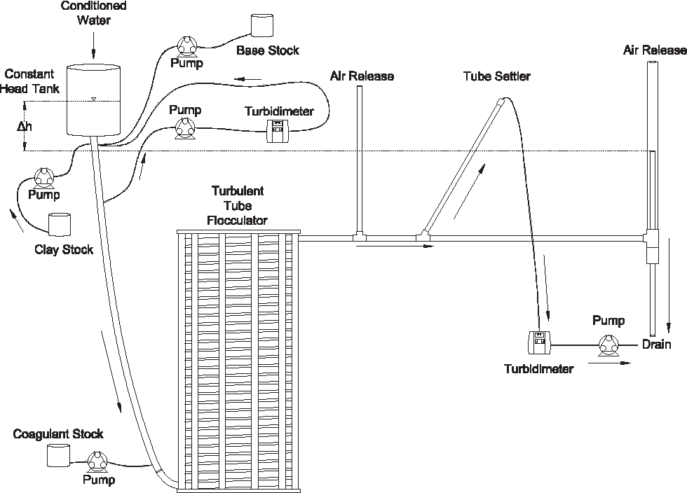
Primary particles are chosen over the minimally settleable size or any intermediate nonsettleable size, because it is hypothesized that, since primary particles must collide with other small nonsettleable particles numerous times to attain a settleable size, collisions involving primary particles are the rate-limiting step in flocculation. For the majority of the flocculation process in an initially monodisperse suspension, after the first collisions have been completed, the collision rate of primary particles becomes slower than the collision rates of an equivalent number concentration of primary particles that have already formed flocs containing any other number of primary particles (Weber-Shirk and Lion, 2010). Therefore, the final concentration of nonsettleable particles is dependent upon the collisions of primary particles, and it is hypothesized that the final concentration of nonsettleable particles is proportional to the final concentration of primary particles. Further experimental work will be needed to confirm this hypothesis and detail this relationship, but for this study, prediction of performance with respect to primary particles will be considered representative of nonsettleable particles. The primary particles are defined here as the suspended particles (kaolinite for this study) and the attached nanoparticles of coagulant precipitate.
Viscous model derivation
Solving Equation (12) for \documentclass{aastex}\usepackage{amsbsy}\usepackage{amsfonts}\usepackage{amssymb}\usepackage{bm}\usepackage{mathrsfs}\usepackage{pifont}\usepackage{stmaryrd}\usepackage{textcomp}\usepackage{portland, xspace}\usepackage{amsmath, amsxtra}\usepackage{upgreek}\pagestyle{empty}\DeclareMathSizes{10}{9}{7}{6}\begin{document}
$${ \rm{d}}{N_{ \rm{c}}}$$
\end{document}, substituting it into Equations (10) and (11), and rewriting the equations in terms of primary particles result in Equation (13):
\documentclass{aastex}\usepackage{amsbsy}\usepackage{amsfonts}\usepackage{amssymb}\usepackage{bm}\usepackage{mathrsfs}\usepackage{pifont}\usepackage{stmaryrd}\usepackage{textcomp}\usepackage{portland, xspace}\usepackage{amsmath, amsxtra}\usepackage{upgreek}\pagestyle{empty}\DeclareMathSizes{10}{9}{7}{6}\begin{document}
\begin{align*}
{ \frac { { \rm d } { C_ { \rm P } } } { - k { C_ { \rm P } } } } = \pi \bar \alpha { \left( { \frac { 6 } { \pi } { \frac { { C_ { \rm P } } } { { \rho _ { \rm P } } } } } \right) ^ { 2 / 3 } } \bar G { \rm { d } } t , \tag { 13 }
\end{align*}
\end{document}
From this point forward, variables with the subscript P will represent a property of the primary particle subset of the nonsettleable particle population rather than the whole.
It is interesting to note that rearranging Equations (13) and (14) in terms of \documentclass{aastex}\usepackage{amsbsy}\usepackage{amsfonts}\usepackage{amssymb}\usepackage{bm}\usepackage{mathrsfs}\usepackage{pifont}\usepackage{stmaryrd}\usepackage{textcomp}\usepackage{portland, xspace}\usepackage{amsmath, amsxtra}\usepackage{upgreek}\pagestyle{empty}\DeclareMathSizes{10}{9}{7}{6}\begin{document}
$$ { \frac { { \rm d } { C_ { \rm P } } } { { \rm d } t } } $$
\end{document} gives exponents for \documentclass{aastex}\usepackage{amsbsy}\usepackage{amsfonts}\usepackage{amssymb}\usepackage{bm}\usepackage{mathrsfs}\usepackage{pifont}\usepackage{stmaryrd}\usepackage{textcomp}\usepackage{portland, xspace}\usepackage{amsmath, amsxtra}\usepackage{upgreek}\pagestyle{empty}\DeclareMathSizes{10}{9}{7}{6}\begin{document}
$${C_{ \rm{P}}}$$
\end{document} of \documentclass{aastex}\usepackage{amsbsy}\usepackage{amsfonts}\usepackage{amssymb}\usepackage{bm}\usepackage{mathrsfs}\usepackage{pifont}\usepackage{stmaryrd}\usepackage{textcomp}\usepackage{portland, xspace}\usepackage{amsmath, amsxtra}\usepackage{upgreek}\pagestyle{empty}\DeclareMathSizes{10}{9}{7}{6}\begin{document}
$$ \frac { 5 } { 3 } $$
\end{document} and \documentclass{aastex}\usepackage{amsbsy}\usepackage{amsfonts}\usepackage{amssymb}\usepackage{bm}\usepackage{mathrsfs}\usepackage{pifont}\usepackage{stmaryrd}\usepackage{textcomp}\usepackage{portland, xspace}\usepackage{amsmath, amsxtra}\usepackage{upgreek}\pagestyle{empty}\DeclareMathSizes{10}{9}{7}{6}\begin{document}
$$ \frac { { 17 } } { 9 } $$
\end{document}. Previous flocculation rate equations were second order, but the observed flocculation rate was less than second order (Benjamin and Lawler, 2013). The slight deviation from an exponent of two comes from the assumption of Pennock et al. (2016) that relative velocity between colliding particles scales with \documentclass{aastex}\usepackage{amsbsy}\usepackage{amsfonts}\usepackage{amssymb}\usepackage{bm}\usepackage{mathrsfs}\usepackage{pifont}\usepackage{stmaryrd}\usepackage{textcomp}\usepackage{portland, xspace}\usepackage{amsmath, amsxtra}\usepackage{upgreek}\pagestyle{empty}\DeclareMathSizes{10}{9}{7}{6}\begin{document}
$${ \rm{ \Lambda }}$$
\end{document} rather than \documentclass{aastex}\usepackage{amsbsy}\usepackage{amsfonts}\usepackage{amssymb}\usepackage{bm}\usepackage{mathrsfs}\usepackage{pifont}\usepackage{stmaryrd}\usepackage{textcomp}\usepackage{portland, xspace}\usepackage{amsmath, amsxtra}\usepackage{upgreek}\pagestyle{empty}\DeclareMathSizes{10}{9}{7}{6}\begin{document}
$${d_{ \rm{P}}}$$
\end{document}. This is to say that, in dilute suspensions characteristic of raw water, where particles are separated by \documentclass{aastex}\usepackage{amsbsy}\usepackage{amsfonts}\usepackage{amssymb}\usepackage{bm}\usepackage{mathrsfs}\usepackage{pifont}\usepackage{stmaryrd}\usepackage{textcomp}\usepackage{portland, xspace}\usepackage{amsmath, amsxtra}\usepackage{upgreek}\pagestyle{empty}\DeclareMathSizes{10}{9}{7}{6}\begin{document}
$${ \rm{ \overline \Lambda }} \gg { \overline d_{ \rm{P}}}$$
\end{document}, the majority of \documentclass{aastex}\usepackage{amsbsy}\usepackage{amsfonts}\usepackage{amssymb}\usepackage{bm}\usepackage{mathrsfs}\usepackage{pifont}\usepackage{stmaryrd}\usepackage{textcomp}\usepackage{portland, xspace}\usepackage{amsmath, amsxtra}\usepackage{upgreek}\pagestyle{empty}\DeclareMathSizes{10}{9}{7}{6}\begin{document}
$$\overline {{t_{ \rm{c}}}}$$
\end{document} is spent with the distance between particles characterized by \documentclass{aastex}\usepackage{amsbsy}\usepackage{amsfonts}\usepackage{amssymb}\usepackage{bm}\usepackage{mathrsfs}\usepackage{pifont}\usepackage{stmaryrd}\usepackage{textcomp}\usepackage{portland, xspace}\usepackage{amsmath, amsxtra}\usepackage{upgreek}\pagestyle{empty}\DeclareMathSizes{10}{9}{7}{6}\begin{document}
$${ \rm{ \overline \Lambda }}$$
\end{document} instead of \documentclass{aastex}\usepackage{amsbsy}\usepackage{amsfonts}\usepackage{amssymb}\usepackage{bm}\usepackage{mathrsfs}\usepackage{pifont}\usepackage{stmaryrd}\usepackage{textcomp}\usepackage{portland, xspace}\usepackage{amsmath, amsxtra}\usepackage{upgreek}\pagestyle{empty}\DeclareMathSizes{10}{9}{7}{6}\begin{document}
$${ \overline d_{ \rm{P}}}$$
\end{document}. The time required for the final approach for a collision is hypothesized to be insignificant compared to the time for \documentclass{aastex}\usepackage{amsbsy}\usepackage{amsfonts}\usepackage{amssymb}\usepackage{bm}\usepackage{mathrsfs}\usepackage{pifont}\usepackage{stmaryrd}\usepackage{textcomp}\usepackage{portland, xspace}\usepackage{amsmath, amsxtra}\usepackage{upgreek}\pagestyle{empty}\DeclareMathSizes{10}{9}{7}{6}\begin{document}
$${ \overline V_{{ \rm{Cleared}}}}$$
\end{document} to equal \documentclass{aastex}\usepackage{amsbsy}\usepackage{amsfonts}\usepackage{amssymb}\usepackage{bm}\usepackage{mathrsfs}\usepackage{pifont}\usepackage{stmaryrd}\usepackage{textcomp}\usepackage{portland, xspace}\usepackage{amsmath, amsxtra}\usepackage{upgreek}\pagestyle{empty}\DeclareMathSizes{10}{9}{7}{6}\begin{document}
$${ \overline V_{{ \rm{Surround}}}}$$
\end{document}.
From Equations (13) and (14), it is possible to integrate and obtain equations for flocculation performance. After separation of variables, one side of the equation is integrated with respect to time from the initial time \documentclass{aastex}\usepackage{amsbsy}\usepackage{amsfonts}\usepackage{amssymb}\usepackage{bm}\usepackage{mathrsfs}\usepackage{pifont}\usepackage{stmaryrd}\usepackage{textcomp}\usepackage{portland, xspace}\usepackage{amsmath, amsxtra}\usepackage{upgreek}\pagestyle{empty}\DeclareMathSizes{10}{9}{7}{6}\begin{document}
$$( t = 0 )$$
\end{document} to the time of interest, generally taken to be the mean hydraulic residence time \documentclass{aastex}\usepackage{amsbsy}\usepackage{amsfonts}\usepackage{amssymb}\usepackage{bm}\usepackage{mathrsfs}\usepackage{pifont}\usepackage{stmaryrd}\usepackage{textcomp}\usepackage{portland, xspace}\usepackage{amsmath, amsxtra}\usepackage{upgreek}\pagestyle{empty}\DeclareMathSizes{10}{9}{7}{6}\begin{document}
$$( t = \theta )$$
\end{document}. The other side of the equation is integrated with respect to the concentration of primary particles from the value at the initial time \documentclass{aastex}\usepackage{amsbsy}\usepackage{amsfonts}\usepackage{amssymb}\usepackage{bm}\usepackage{mathrsfs}\usepackage{pifont}\usepackage{stmaryrd}\usepackage{textcomp}\usepackage{portland, xspace}\usepackage{amsmath, amsxtra}\usepackage{upgreek}\pagestyle{empty}\DeclareMathSizes{10}{9}{7}{6}\begin{document}
$$( {C_{{{ \rm{P}}_0}}} )$$
\end{document}, equivalent to the initial concentration of nonsettleable particles, to the concentration of primary particles at the time of interest \documentclass{aastex}\usepackage{amsbsy}\usepackage{amsfonts}\usepackage{amssymb}\usepackage{bm}\usepackage{mathrsfs}\usepackage{pifont}\usepackage{stmaryrd}\usepackage{textcomp}\usepackage{portland, xspace}\usepackage{amsmath, amsxtra}\usepackage{upgreek}\pagestyle{empty}\DeclareMathSizes{10}{9}{7}{6}\begin{document}
$$( {C_{ \rm{P}}} )$$
\end{document}. For collisions dominated by viscous forces [Eq. (13)], the integral becomes as follows:
\documentclass{aastex}\usepackage{amsbsy}\usepackage{amsfonts}\usepackage{amssymb}\usepackage{bm}\usepackage{mathrsfs}\usepackage{pifont}\usepackage{stmaryrd}\usepackage{textcomp}\usepackage{portland, xspace}\usepackage{amsmath, amsxtra}\usepackage{upgreek}\pagestyle{empty}\DeclareMathSizes{10}{9}{7}{6}\begin{document}
\begin{align*}
\frac { 1 } { \pi } { \left( { { \rho _ { \rm { P } } } \frac { \pi } { 6 } } \right) ^ { 2 / 3 } } \mathop \smallint \limits_ { { C_ { { { \rm { P } } _0 } } } } ^ { { C_ { \rm { P } } } } C_ { \rm { P } } ^ { - 5 / 3 } { \rm { d } } { C_ { \rm { P } } } = - k \bar \alpha \bar G \mathop \smallint \limits_0^ \theta { \rm { d } } t. \tag { 15 }
\end{align*}
\end{document}
The integral on the left-hand side assumes that \documentclass{aastex}\usepackage{amsbsy}\usepackage{amsfonts}\usepackage{amssymb}\usepackage{bm}\usepackage{mathrsfs}\usepackage{pifont}\usepackage{stmaryrd}\usepackage{textcomp}\usepackage{portland, xspace}\usepackage{amsmath, amsxtra}\usepackage{upgreek}\pagestyle{empty}\DeclareMathSizes{10}{9}{7}{6}\begin{document}
$${ \rho _{ \rm{P}}}$$
\end{document} does not change as \documentclass{aastex}\usepackage{amsbsy}\usepackage{amsfonts}\usepackage{amssymb}\usepackage{bm}\usepackage{mathrsfs}\usepackage{pifont}\usepackage{stmaryrd}\usepackage{textcomp}\usepackage{portland, xspace}\usepackage{amsmath, amsxtra}\usepackage{upgreek}\pagestyle{empty}\DeclareMathSizes{10}{9}{7}{6}\begin{document}
$${C_{ \rm{P}}}$$
\end{document} changes. One assumption on the right side is that \documentclass{aastex}\usepackage{amsbsy}\usepackage{amsfonts}\usepackage{amssymb}\usepackage{bm}\usepackage{mathrsfs}\usepackage{pifont}\usepackage{stmaryrd}\usepackage{textcomp}\usepackage{portland, xspace}\usepackage{amsmath, amsxtra}\usepackage{upgreek}\pagestyle{empty}\DeclareMathSizes{10}{9}{7}{6}\begin{document}
$${ \rm{ \overline \Gamma }}$$
\end{document}, of which \documentclass{aastex}\usepackage{amsbsy}\usepackage{amsfonts}\usepackage{amssymb}\usepackage{bm}\usepackage{mathrsfs}\usepackage{pifont}\usepackage{stmaryrd}\usepackage{textcomp}\usepackage{portland, xspace}\usepackage{amsmath, amsxtra}\usepackage{upgreek}\pagestyle{empty}\DeclareMathSizes{10}{9}{7}{6}\begin{document}
$$\bar \alpha$$
\end{document} is a function, does not vary with t. This requires that attachment of coagulant to colloidal particles in rapid mix be fast enough to be approximated as completed by the beginning of flocculation. This assumption may not be valid for high rate flocculators, especially under conditions of low \documentclass{aastex}\usepackage{amsbsy}\usepackage{amsfonts}\usepackage{amssymb}\usepackage{bm}\usepackage{mathrsfs}\usepackage{pifont}\usepackage{stmaryrd}\usepackage{textcomp}\usepackage{portland, xspace}\usepackage{amsmath, amsxtra}\usepackage{upgreek}\pagestyle{empty}\DeclareMathSizes{10}{9}{7}{6}\begin{document}
$${C_{{{ \rm{P}}_0}}}$$
\end{document}. Further work on the rate and efficacy of rapid mix is merited.
The other assumption on the right-hand side is that the mean velocity gradient, \documentclass{aastex}\usepackage{amsbsy}\usepackage{amsfonts}\usepackage{amssymb}\usepackage{bm}\usepackage{mathrsfs}\usepackage{pifont}\usepackage{stmaryrd}\usepackage{textcomp}\usepackage{portland, xspace}\usepackage{amsmath, amsxtra}\usepackage{upgreek}\pagestyle{empty}\DeclareMathSizes{10}{9}{7}{6}\begin{document}
$$\overline G$$
\end{document}, does not change over the course of the flocculation process. In mechanically mixed flocculators, the use of a simple spatial average is not reasonable, as the velocity gradient changes very dramatically from the bulk flow to the tip of the impeller blade and individual particles follow different paths that expose them to different velocity gradient zones in different sequences and durations (Boller and Blaser, 1998). The distribution of residence times in a mechanical flocculator would also need to be taken into account for the integration. For baffled hydraulic flocculators, on the other hand, the use of the spatial average, \documentclass{aastex}\usepackage{amsbsy}\usepackage{amsfonts}\usepackage{amssymb}\usepackage{bm}\usepackage{mathrsfs}\usepackage{pifont}\usepackage{stmaryrd}\usepackage{textcomp}\usepackage{portland, xspace}\usepackage{amsmath, amsxtra}\usepackage{upgreek}\pagestyle{empty}\DeclareMathSizes{10}{9}{7}{6}\begin{document}
$$\overline G$$
\end{document}, and considering it constant with t is generally a reasonable approach. This is because mixing energy in a well-designed hydraulic flocculator is rather uniformly distributed spatially, the zones of higher energy dissipation rate after the baffles do not vary appreciably with time when operating at a constant flow rate, and all particles follow similar paths through the flocculator.
This can be put in terms of \documentclass{aastex}\usepackage{amsbsy}\usepackage{amsfonts}\usepackage{amssymb}\usepackage{bm}\usepackage{mathrsfs}\usepackage{pifont}\usepackage{stmaryrd}\usepackage{textcomp}\usepackage{portland, xspace}\usepackage{amsmath, amsxtra}\usepackage{upgreek}\pagestyle{empty}\DeclareMathSizes{10}{9}{7}{6}\begin{document}
$${ \rm{ \overline \Lambda }}$$
\end{document} for simplicity by using Equation (9) and rearranging in terms of the familiar Camp-Stein parameter, \documentclass{aastex}\usepackage{amsbsy}\usepackage{amsfonts}\usepackage{amssymb}\usepackage{bm}\usepackage{mathrsfs}\usepackage{pifont}\usepackage{stmaryrd}\usepackage{textcomp}\usepackage{portland, xspace}\usepackage{amsmath, amsxtra}\usepackage{upgreek}\pagestyle{empty}\DeclareMathSizes{10}{9}{7}{6}\begin{document}
$$\overline G \theta$$
\end{document}, to be as follows:
\documentclass{aastex}\usepackage{amsbsy}\usepackage{amsfonts}\usepackage{amssymb}\usepackage{bm}\usepackage{mathrsfs}\usepackage{pifont}\usepackage{stmaryrd}\usepackage{textcomp}\usepackage{portland, xspace}\usepackage{amsmath, amsxtra}\usepackage{upgreek}\pagestyle{empty}\DeclareMathSizes{10}{9}{7}{6}\begin{document}
\begin{align*}
\overline G \theta = \frac { 3 } { 2 } { \frac { \left( { { { { \rm { \overline \Lambda } } } ^2 } - { \rm { \overline \Lambda } } _0^2 } \right) } { k \pi \bar \alpha \bar d_ { \rm P } ^2 } } , \tag { 17 }
\end{align*}
\end{document}
which is the final form of the viscous flocculation design equation. Equation (17) gives guidance for flocculator design in that higher values of \documentclass{aastex}\usepackage{amsbsy}\usepackage{amsfonts}\usepackage{amssymb}\usepackage{bm}\usepackage{mathrsfs}\usepackage{pifont}\usepackage{stmaryrd}\usepackage{textcomp}\usepackage{portland, xspace}\usepackage{amsmath, amsxtra}\usepackage{upgreek}\pagestyle{empty}\DeclareMathSizes{10}{9}{7}{6}\begin{document}
$$\overline G \theta$$
\end{document} are needed for flocculators to achieve greater changes in \documentclass{aastex}\usepackage{amsbsy}\usepackage{amsfonts}\usepackage{amssymb}\usepackage{bm}\usepackage{mathrsfs}\usepackage{pifont}\usepackage{stmaryrd}\usepackage{textcomp}\usepackage{portland, xspace}\usepackage{amsmath, amsxtra}\usepackage{upgreek}\pagestyle{empty}\DeclareMathSizes{10}{9}{7}{6}\begin{document}
$${ \rm{ \overline \Lambda }}$$
\end{document} (or \documentclass{aastex}\usepackage{amsbsy}\usepackage{amsfonts}\usepackage{amssymb}\usepackage{bm}\usepackage{mathrsfs}\usepackage{pifont}\usepackage{stmaryrd}\usepackage{textcomp}\usepackage{portland, xspace}\usepackage{amsmath, amsxtra}\usepackage{upgreek}\pagestyle{empty}\DeclareMathSizes{10}{9}{7}{6}\begin{document}
$${C_{ \rm{P}}}$$
\end{document}) or to overcome low \documentclass{aastex}\usepackage{amsbsy}\usepackage{amsfonts}\usepackage{amssymb}\usepackage{bm}\usepackage{mathrsfs}\usepackage{pifont}\usepackage{stmaryrd}\usepackage{textcomp}\usepackage{portland, xspace}\usepackage{amsmath, amsxtra}\usepackage{upgreek}\pagestyle{empty}\DeclareMathSizes{10}{9}{7}{6}\begin{document}
$${ \rm{ \overline \Gamma }}$$
\end{document}. It should be noted that the \documentclass{aastex}\usepackage{amsbsy}\usepackage{amsfonts}\usepackage{amssymb}\usepackage{bm}\usepackage{mathrsfs}\usepackage{pifont}\usepackage{stmaryrd}\usepackage{textcomp}\usepackage{portland, xspace}\usepackage{amsmath, amsxtra}\usepackage{upgreek}\pagestyle{empty}\DeclareMathSizes{10}{9}{7}{6}\begin{document}
$${{ \rm{ \bar \Lambda }}_0}$$
\end{document} term in Equation (17) will generally be very small compared to the \documentclass{aastex}\usepackage{amsbsy}\usepackage{amsfonts}\usepackage{amssymb}\usepackage{bm}\usepackage{mathrsfs}\usepackage{pifont}\usepackage{stmaryrd}\usepackage{textcomp}\usepackage{portland, xspace}\usepackage{amsmath, amsxtra}\usepackage{upgreek}\pagestyle{empty}\DeclareMathSizes{10}{9}{7}{6}\begin{document}
$${ \rm{ \overline \Lambda }}$$
\end{document} term for most flocculation scenarios. In this case, \documentclass{aastex}\usepackage{amsbsy}\usepackage{amsfonts}\usepackage{amssymb}\usepackage{bm}\usepackage{mathrsfs}\usepackage{pifont}\usepackage{stmaryrd}\usepackage{textcomp}\usepackage{portland, xspace}\usepackage{amsmath, amsxtra}\usepackage{upgreek}\pagestyle{empty}\DeclareMathSizes{10}{9}{7}{6}\begin{document}
$${{ \rm{ \overline \Lambda }}_0}$$
\end{document} can be considered negligible. While simplifying the equation, it also gives the result that flocculators must be designed not so much for the particle concentrations they will receive, but for the particle concentrations they are intended to produce. Modifying Equation (17) to be in terms of \documentclass{aastex}\usepackage{amsbsy}\usepackage{amsfonts}\usepackage{amssymb}\usepackage{bm}\usepackage{mathrsfs}\usepackage{pifont}\usepackage{stmaryrd}\usepackage{textcomp}\usepackage{portland, xspace}\usepackage{amsmath, amsxtra}\usepackage{upgreek}\pagestyle{empty}\DeclareMathSizes{10}{9}{7}{6}\begin{document}
$${C_{ \rm{P}}}$$
\end{document} produces the following equation:
\documentclass{aastex}\usepackage{amsbsy}\usepackage{amsfonts}\usepackage{amssymb}\usepackage{bm}\usepackage{mathrsfs}\usepackage{pifont}\usepackage{stmaryrd}\usepackage{textcomp}\usepackage{portland, xspace}\usepackage{amsmath, amsxtra}\usepackage{upgreek}\pagestyle{empty}\DeclareMathSizes{10}{9}{7}{6}\begin{document}
\begin{align*}
\overline G \theta = \frac { 3 } { { 2k \pi \bar \alpha } } { \left( { \frac { \pi } { 6 } { \frac { { \rho _ { \rm P } } } { { C_ { \rm P } } } } } \right) ^ { 2 / 3 } } . \tag { 18 }
\end{align*}
\end{document}
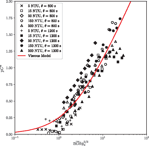
A desirable way to represent flocculation performance is with the negative log of the fraction of particles remaining (also often referred to as log removal), \documentclass{aastex}\usepackage{amsbsy}\usepackage{amsfonts}\usepackage{amssymb}\usepackage{bm}\usepackage{mathrsfs}\usepackage{pifont}\usepackage{stmaryrd}\usepackage{textcomp}\usepackage{portland, xspace}\usepackage{amsmath, amsxtra}\usepackage{upgreek}\pagestyle{empty}\DeclareMathSizes{10}{9}{7}{6}\begin{document}
$${ \rm{p}}{C^*}$$
\end{document}, given in Swetland et al. (2014) as follows:
\documentclass{aastex}\usepackage{amsbsy}\usepackage{amsfonts}\usepackage{amssymb}\usepackage{bm}\usepackage{mathrsfs}\usepackage{pifont}\usepackage{stmaryrd}\usepackage{textcomp}\usepackage{portland, xspace}\usepackage{amsmath, amsxtra}\usepackage{upgreek}\pagestyle{empty}\DeclareMathSizes{10}{9}{7}{6}\begin{document}
\begin{align*}
{ \rm { p } } { C^* } = - { \log _ { 10 } } \left( { { \frac { { C_ { \rm P } } } { { C_ { { { \rm P } _0 } } } } } } \right) \tag { 19 }
\end{align*}
\end{document}
Likewise, a way to simplify Equation (16) is to put it in terms of the particle volume fraction, \documentclass{aastex}\usepackage{amsbsy}\usepackage{amsfonts}\usepackage{amssymb}\usepackage{bm}\usepackage{mathrsfs}\usepackage{pifont}\usepackage{stmaryrd}\usepackage{textcomp}\usepackage{portland, xspace}\usepackage{amsmath, amsxtra}\usepackage{upgreek}\pagestyle{empty}\DeclareMathSizes{10}{9}{7}{6}\begin{document}
$$\phi$$
\end{document}, defined as follows:
\documentclass{aastex}\usepackage{amsbsy}\usepackage{amsfonts}\usepackage{amssymb}\usepackage{bm}\usepackage{mathrsfs}\usepackage{pifont}\usepackage{stmaryrd}\usepackage{textcomp}\usepackage{portland, xspace}\usepackage{amsmath, amsxtra}\usepackage{upgreek}\pagestyle{empty}\DeclareMathSizes{10}{9}{7}{6}\begin{document}
\begin{align*}
\phi = { \frac { { C_ { \rm P } } } { { \rho _ { \rm P } } } } = \frac { \pi } { 6 } { \left( { { \frac { { { \overline d } _ { \rm P } } } { { \rm { \overline \Lambda } } } } } \right) ^3 } . \tag { 20 }
\end{align*}
\end{document}
which is the viscous flocculation operation equation.
The AguaClara viscous flocculation operation equation is a predictive performance relationship for flocculation in flows with long range particle transport toward collisions dominated by viscous forces. It is proposed as applicable to laminar flows, with potential applicability to the dissipation range of turbulent flows. Given the properties of the flocculator (\documentclass{aastex}\usepackage{amsbsy}\usepackage{amsfonts}\usepackage{amssymb}\usepackage{bm}\usepackage{mathrsfs}\usepackage{pifont}\usepackage{stmaryrd}\usepackage{textcomp}\usepackage{portland, xspace}\usepackage{amsmath, amsxtra}\usepackage{upgreek}\pagestyle{empty}\DeclareMathSizes{10}{9}{7}{6}\begin{document}
$$\overline G \, \,{ \rm and} \, \, \theta$$
\end{document}) and its influent (\documentclass{aastex}\usepackage{amsbsy}\usepackage{amsfonts}\usepackage{amssymb}\usepackage{bm}\usepackage{mathrsfs}\usepackage{pifont}\usepackage{stmaryrd}\usepackage{textcomp}\usepackage{portland, xspace}\usepackage{amsmath, amsxtra}\usepackage{upgreek}\pagestyle{empty}\DeclareMathSizes{10}{9}{7}{6}\begin{document}
$${ \phi _0} \, \,{\rm and} \, \, \bar \alpha$$
\end{document}), flocculation performance can be predicted in terms of \documentclass{aastex}\usepackage{amsbsy}\usepackage{amsfonts}\usepackage{amssymb}\usepackage{bm}\usepackage{mathrsfs}\usepackage{pifont}\usepackage{stmaryrd}\usepackage{textcomp}\usepackage{portland, xspace}\usepackage{amsmath, amsxtra}\usepackage{upgreek}\pagestyle{empty}\DeclareMathSizes{10}{9}{7}{6}\begin{document}
$${ \rm{p}}{C^*}$$
\end{document}. The development of the design and operation equations, Equations (17) and (21), was the result of a team effort of Cornell University's AguaClara program and hence they will subsequently be referred to collectively as the AguaClara viscous flocculation model.
Inertial model derivation
The same procedure that was used to find Equation (21) for viscous-dominated flocculation can be performed on Equation (14) for flocculation predominantly controlled by inertial forces. Once the variables are separated, the integration is set up as follows:
\documentclass{aastex}\usepackage{amsbsy}\usepackage{amsfonts}\usepackage{amssymb}\usepackage{bm}\usepackage{mathrsfs}\usepackage{pifont}\usepackage{stmaryrd}\usepackage{textcomp}\usepackage{portland, xspace}\usepackage{amsmath, amsxtra}\usepackage{upgreek}\pagestyle{empty}\DeclareMathSizes{10}{9}{7}{6}\begin{document}
\begin{align*}
\frac { 1 } { \pi } { \left( { \frac { \pi } { 6 } { \rho _ { \rm { P } } } } \right) ^ { 8 / 9 } } \mathop \smallint \limits_ { { C_ { { { \rm { P } } _0 } } } } ^ { { C_ { \rm { P } } } } C_ { \rm { P } } ^ { - 17 / 9 } { \rm { d } } { C_ { \rm { P } } } = - k \bar \alpha { \left( { { \frac { \bar \varepsilon } { \bar d_P^2 } } } \right) ^ { 1 / 3 } } \mathop \smallint \limits_0^\theta { \rm { d } } t. \tag { 22 }
\end{align*}
\end{document}
This integration makes the same assumptions as those given for Equation (15) with the additional assumption that \documentclass{aastex}\usepackage{amsbsy}\usepackage{amsfonts}\usepackage{amssymb}\usepackage{bm}\usepackage{mathrsfs}\usepackage{pifont}\usepackage{stmaryrd}\usepackage{textcomp}\usepackage{portland, xspace}\usepackage{amsmath, amsxtra}\usepackage{upgreek}\pagestyle{empty}\DeclareMathSizes{10}{9}{7}{6}\begin{document}
$${ \bar d_{ \rm{P}}}$$
\end{document} does not vary with t.
As previously, the integrated result can be rearranged to provide more design intuition. The alternate form, which is analogous to Equation (17), is as follows:
\documentclass{aastex}\usepackage{amsbsy}\usepackage{amsfonts}\usepackage{amssymb}\usepackage{bm}\usepackage{mathrsfs}\usepackage{pifont}\usepackage{stmaryrd}\usepackage{textcomp}\usepackage{portland, xspace}\usepackage{amsmath, amsxtra}\usepackage{upgreek}\pagestyle{empty}\DeclareMathSizes{10}{9}{7}{6}\begin{document}
\begin{align*}
{ \bar \varepsilon ^ { 1 / 3 } } \theta = \frac { 9 } { 8 } { \frac { \left( { { { { \rm { \overline \Lambda } } } ^ { \,8 / 3 } } - { \rm { \overline \Lambda } } _0^ { \,8 / 3 } } \right) } { k \pi \bar \alpha \bar d_ { \rm P } ^2 } } , \tag { 24 }
\end{align*}
\end{document}
which is the inertial flocculation design equation. It should be noted that flocculator design parameter becomes \documentclass{aastex}\usepackage{amsbsy}\usepackage{amsfonts}\usepackage{amssymb}\usepackage{bm}\usepackage{mathrsfs}\usepackage{pifont}\usepackage{stmaryrd}\usepackage{textcomp}\usepackage{portland, xspace}\usepackage{amsmath, amsxtra}\usepackage{upgreek}\pagestyle{empty}\DeclareMathSizes{10}{9}{7}{6}\begin{document}
$${ \bar \varepsilon ^{1 / 3}} \theta$$
\end{document} instead of the Camp-Stein number, \documentclass{aastex}\usepackage{amsbsy}\usepackage{amsfonts}\usepackage{amssymb}\usepackage{bm}\usepackage{mathrsfs}\usepackage{pifont}\usepackage{stmaryrd}\usepackage{textcomp}\usepackage{portland, xspace}\usepackage{amsmath, amsxtra}\usepackage{upgreek}\pagestyle{empty}\DeclareMathSizes{10}{9}{7}{6}\begin{document}
$$\overline G \theta$$
\end{document}, for flocculators in which inertial forces dominate viscous forces in bringing primary particles together for collisions. As before, the form of Equation (24) can also be simplified to be in terms of \documentclass{aastex}\usepackage{amsbsy}\usepackage{amsfonts}\usepackage{amssymb}\usepackage{bm}\usepackage{mathrsfs}\usepackage{pifont}\usepackage{stmaryrd}\usepackage{textcomp}\usepackage{portland, xspace}\usepackage{amsmath, amsxtra}\usepackage{upgreek}\pagestyle{empty}\DeclareMathSizes{10}{9}{7}{6}\begin{document}
$${C_{ \rm{P}}}$$
\end{document} if \documentclass{aastex}\usepackage{amsbsy}\usepackage{amsfonts}\usepackage{amssymb}\usepackage{bm}\usepackage{mathrsfs}\usepackage{pifont}\usepackage{stmaryrd}\usepackage{textcomp}\usepackage{portland, xspace}\usepackage{amsmath, amsxtra}\usepackage{upgreek}\pagestyle{empty}\DeclareMathSizes{10}{9}{7}{6}\begin{document}
$${{ \rm{ \bar \Lambda }}_0}$$
\end{document} is small enough (\documentclass{aastex}\usepackage{amsbsy}\usepackage{amsfonts}\usepackage{amssymb}\usepackage{bm}\usepackage{mathrsfs}\usepackage{pifont}\usepackage{stmaryrd}\usepackage{textcomp}\usepackage{portland, xspace}\usepackage{amsmath, amsxtra}\usepackage{upgreek}\pagestyle{empty}\DeclareMathSizes{10}{9}{7}{6}\begin{document}
$${C_{{{ \rm{P}}_0}}}$$
\end{document} is large enough) to be neglected. For inertially dominated flocculation, this results in the following equation:
\documentclass{aastex}\usepackage{amsbsy}\usepackage{amsfonts}\usepackage{amssymb}\usepackage{bm}\usepackage{mathrsfs}\usepackage{pifont}\usepackage{stmaryrd}\usepackage{textcomp}\usepackage{portland, xspace}\usepackage{amsmath, amsxtra}\usepackage{upgreek}\pagestyle{empty}\DeclareMathSizes{10}{9}{7}{6}\begin{document}
\begin{align*}
{ \bar \varepsilon ^ { 1 / 3 } } \theta = { \frac { 9 \bar d_ { \rm P } ^ { 2 / 3 } } { 8k \pi \bar \alpha } } { \left( { \frac { \pi } { 6 } { \frac { { \rho _ { \rm P } } } { { C_ { \rm P } } } } } \right) ^ { 8 / 9 } } , \tag { 25 }
\end{align*}
\end{document}
Taking the negative logarithm (base 10) of both sides of Equation (23), as before, results in the integral flocculation model for turbulent flows where interparticle collisions are primarily driven by inertia:
\documentclass{aastex}\usepackage{amsbsy}\usepackage{amsfonts}\usepackage{amssymb}\usepackage{bm}\usepackage{mathrsfs}\usepackage{pifont}\usepackage{stmaryrd}\usepackage{textcomp}\usepackage{portland, xspace}\usepackage{amsmath, amsxtra}\usepackage{upgreek}\pagestyle{empty}\DeclareMathSizes{10}{9}{7}{6}\begin{document}
\begin{align*}
{ \rm { p } } { C^* } = \frac { 9 } { 8 } { \log _ { 10 } } \left[ { \frac { 8 } { 9 } { { \left( { \frac { 6 } { \pi } } \right) } ^ { 8 / 9 } } \pi k \bar \alpha { { \left( { { \frac { \bar \varepsilon } { \bar d_P^2 } } } \right) } ^ { 1 / 3 } } \theta \phi _0^ { 8 / 9 } + 1 } \right] , \tag { 26 }
\end{align*}
\end{document}
the inertial flocculation operation equation.
Equation (26) is, like Equation (21), an equation for predicting the performance of a flocculator using known information about the flocculator (\documentclass{aastex}\usepackage{amsbsy}\usepackage{amsfonts}\usepackage{amssymb}\usepackage{bm}\usepackage{mathrsfs}\usepackage{pifont}\usepackage{stmaryrd}\usepackage{textcomp}\usepackage{portland, xspace}\usepackage{amsmath, amsxtra}\usepackage{upgreek}\pagestyle{empty}\DeclareMathSizes{10}{9}{7}{6}\begin{document}
$$\bar \varepsilon$$
\end{document} and \documentclass{aastex}\usepackage{amsbsy}\usepackage{amsfonts}\usepackage{amssymb}\usepackage{bm}\usepackage{mathrsfs}\usepackage{pifont}\usepackage{stmaryrd}\usepackage{textcomp}\usepackage{portland, xspace}\usepackage{amsmath, amsxtra}\usepackage{upgreek}\pagestyle{empty}\DeclareMathSizes{10}{9}{7}{6}\begin{document}
$$\theta$$
\end{document}) and the influent suspension (\documentclass{aastex}\usepackage{amsbsy}\usepackage{amsfonts}\usepackage{amssymb}\usepackage{bm}\usepackage{mathrsfs}\usepackage{pifont}\usepackage{stmaryrd}\usepackage{textcomp}\usepackage{portland, xspace}\usepackage{amsmath, amsxtra}\usepackage{upgreek}\pagestyle{empty}\DeclareMathSizes{10}{9}{7}{6}\begin{document}
$${ \bar d_{ \rm{P}}}$$
\end{document}, \documentclass{aastex}\usepackage{amsbsy}\usepackage{amsfonts}\usepackage{amssymb}\usepackage{bm}\usepackage{mathrsfs}\usepackage{pifont}\usepackage{stmaryrd}\usepackage{textcomp}\usepackage{portland, xspace}\usepackage{amsmath, amsxtra}\usepackage{upgreek}\pagestyle{empty}\DeclareMathSizes{10}{9}{7}{6}\begin{document}
$$\bar \alpha$$
\end{document}, and \documentclass{aastex}\usepackage{amsbsy}\usepackage{amsfonts}\usepackage{amssymb}\usepackage{bm}\usepackage{mathrsfs}\usepackage{pifont}\usepackage{stmaryrd}\usepackage{textcomp}\usepackage{portland, xspace}\usepackage{amsmath, amsxtra}\usepackage{upgreek}\pagestyle{empty}\DeclareMathSizes{10}{9}{7}{6}\begin{document}
$${ \phi _0}$$
\end{document}). Likewise, its development was also a product of a team effort, and so it, along with Equation (25), will collectively be referred to as the AguaClara inertial flocculation model. As with Equation (21), it must be experimentally validated. For these experiments, the flow through the flocculator must be turbulent, and the relative velocities of particles leading up to collision must be influenced primarily by inertial forces.
Validation of the performance equations [Eqs. (21) and (26)] will require experiments over a range of conditions. For laminar flocculation, data have already been collected by Swetland et al. (2014), and the aptness of Equation (21) can be tested with respect to its predictions for these data. Turbulent flow flocculator performance data can also be compared with data from Swetland et al. (2014) to see if there is any distinguishable difference between performances for these two different conditions.
Since validation of the performance equations for turbulent flows requires flocculation experiments in turbulent conditions, it is important to differentiate which experimental conditions will constitute viscosity-dominated flocculation [Eq. (21)] and which will constitute inertia-dominated flocculation [Eq. (26)]. The distinction is made based on the division between ranges of length scales in turbulent flow. The Kolmogorov microscale (\documentclass{aastex}\usepackage{amsbsy}\usepackage{amsfonts}\usepackage{amssymb}\usepackage{bm}\usepackage{mathrsfs}\usepackage{pifont}\usepackage{stmaryrd}\usepackage{textcomp}\usepackage{portland, xspace}\usepackage{amsmath, amsxtra}\usepackage{upgreek}\pagestyle{empty}\DeclareMathSizes{10}{9}{7}{6}\begin{document}
$$\eta$$
\end{document}) describes the smallest dissipative eddies in a turbulent flow and is defined as follows (Pope, 2000):
\documentclass{aastex}\usepackage{amsbsy}\usepackage{amsfonts}\usepackage{amssymb}\usepackage{bm}\usepackage{mathrsfs}\usepackage{pifont}\usepackage{stmaryrd}\usepackage{textcomp}\usepackage{portland, xspace}\usepackage{amsmath, amsxtra}\usepackage{upgreek}\pagestyle{empty}\DeclareMathSizes{10}{9}{7}{6}\begin{document}
\begin{align*}
\eta = { \left( { \frac { { { \nu ^3 } } } { \varepsilon } } \right) ^ { 1 / 4 } } . \tag { 27 }
\end{align*}
\end{document}
At the Kolmogorov microscale, the Reynolds number defined by the length scale of eddies is 1, which means that inertial and viscous forces are in balance. At this length scale, Equations (4) and (6) predict the same \documentclass{aastex}\usepackage{amsbsy}\usepackage{amsfonts}\usepackage{amssymb}\usepackage{bm}\usepackage{mathrsfs}\usepackage{pifont}\usepackage{stmaryrd}\usepackage{textcomp}\usepackage{portland, xspace}\usepackage{amsmath, amsxtra}\usepackage{upgreek}\pagestyle{empty}\DeclareMathSizes{10}{9}{7}{6}\begin{document}
$${v_{ \rm{r}}}$$
\end{document}, meaning that the successful collision rate for both the viscous and inertial models is the same when \documentclass{aastex}\usepackage{amsbsy}\usepackage{amsfonts}\usepackage{amssymb}\usepackage{bm}\usepackage{mathrsfs}\usepackage{pifont}\usepackage{stmaryrd}\usepackage{textcomp}\usepackage{portland, xspace}\usepackage{amsmath, amsxtra}\usepackage{upgreek}\pagestyle{empty}\DeclareMathSizes{10}{9}{7}{6}\begin{document}
$${ \rm{ \overline \Lambda }} = \bar \eta$$
\end{document}, where \documentclass{aastex}\usepackage{amsbsy}\usepackage{amsfonts}\usepackage{amssymb}\usepackage{bm}\usepackage{mathrsfs}\usepackage{pifont}\usepackage{stmaryrd}\usepackage{textcomp}\usepackage{portland, xspace}\usepackage{amsmath, amsxtra}\usepackage{upgreek}\pagestyle{empty}\DeclareMathSizes{10}{9}{7}{6}\begin{document}
$$\bar \eta$$
\end{document} is the spatially averaged Kolmogorov microscale for the flow.
Therefore, for this study, when \documentclass{aastex}\usepackage{amsbsy}\usepackage{amsfonts}\usepackage{amssymb}\usepackage{bm}\usepackage{mathrsfs}\usepackage{pifont}\usepackage{stmaryrd}\usepackage{textcomp}\usepackage{portland, xspace}\usepackage{amsmath, amsxtra}\usepackage{upgreek}\pagestyle{empty}\DeclareMathSizes{10}{9}{7}{6}\begin{document}
$$ { \frac { { \rm { \overline \Lambda } } } { \bar \eta } } \ge 1$$
\end{document}, flocculation was considered to occur in the inertial subrange, and when \documentclass{aastex}\usepackage{amsbsy}\usepackage{amsfonts}\usepackage{amssymb}\usepackage{bm}\usepackage{mathrsfs}\usepackage{pifont}\usepackage{stmaryrd}\usepackage{textcomp}\usepackage{portland, xspace}\usepackage{amsmath, amsxtra}\usepackage{upgreek}\pagestyle{empty}\DeclareMathSizes{10}{9}{7}{6}\begin{document}
$$ { \frac { { \rm { \overline \Lambda } } } { \bar \eta } } < 1$$
\end{document}, flocculation was nominally said to occur in the dissipation range. Turbulence literature indicates that the transition between the inertial subrange and the dissipation range does not occur at the Kolmogorov microscale, but at some length scale that is a multiple, probably order 10, of the Kolmogorov microscale (Pope, 2000). Dimotakis (2000) suggested that scales greater than \documentclass{aastex}\usepackage{amsbsy}\usepackage{amsfonts}\usepackage{amssymb}\usepackage{bm}\usepackage{mathrsfs}\usepackage{pifont}\usepackage{stmaryrd}\usepackage{textcomp}\usepackage{portland, xspace}\usepackage{amsmath, amsxtra}\usepackage{upgreek}\pagestyle{empty}\DeclareMathSizes{10}{9}{7}{6}\begin{document}
$$50 \eta$$
\end{document} are completely inertial. There does not, however, appear to be a clear value given for this length scale, and for the purposes of this study, the Kolmogorov microscale was utilized to nominally characterize the transition. Experiments to test Equation (21) must therefore occur in conditions where \documentclass{aastex}\usepackage{amsbsy}\usepackage{amsfonts}\usepackage{amssymb}\usepackage{bm}\usepackage{mathrsfs}\usepackage{pifont}\usepackage{stmaryrd}\usepackage{textcomp}\usepackage{portland, xspace}\usepackage{amsmath, amsxtra}\usepackage{upgreek}\pagestyle{empty}\DeclareMathSizes{10}{9}{7}{6}\begin{document}
$$ { \frac { { \rm { \overline \Lambda } } } { \bar \eta } } < 1$$
\end{document}, and experiments to test Equation (26) must occur in conditions where \documentclass{aastex}\usepackage{amsbsy}\usepackage{amsfonts}\usepackage{amssymb}\usepackage{bm}\usepackage{mathrsfs}\usepackage{pifont}\usepackage{stmaryrd}\usepackage{textcomp}\usepackage{portland, xspace}\usepackage{amsmath, amsxtra}\usepackage{upgreek}\pagestyle{empty}\DeclareMathSizes{10}{9}{7}{6}\begin{document}
$$ { \frac { { \rm { \overline \Lambda } } } { \bar \eta } } \ge 1$$
\end{document}.
Based on the considerations given above, there were two potential lines of experimentation to prove the validity of both the AguaClara viscous and AguaClara inertial flocculation models. The applicability of Equation (21) to the dissipation range of turbulent flow required experiments performed in conditions where \documentclass{aastex}\usepackage{amsbsy}\usepackage{amsfonts}\usepackage{amssymb}\usepackage{bm}\usepackage{mathrsfs}\usepackage{pifont}\usepackage{stmaryrd}\usepackage{textcomp}\usepackage{portland, xspace}\usepackage{amsmath, amsxtra}\usepackage{upgreek}\pagestyle{empty}\DeclareMathSizes{10}{9}{7}{6}\begin{document}
$$ { \frac { { \rm { \overline \Lambda } } } { \bar \eta } } $$
\end{document} was small (i.e., \documentclass{aastex}\usepackage{amsbsy}\usepackage{amsfonts}\usepackage{amssymb}\usepackage{bm}\usepackage{mathrsfs}\usepackage{pifont}\usepackage{stmaryrd}\usepackage{textcomp}\usepackage{portland, xspace}\usepackage{amsmath, amsxtra}\usepackage{upgreek}\pagestyle{empty}\DeclareMathSizes{10}{9}{7}{6}\begin{document}
$$< 1$$
\end{document}). This could be accomplished by performing experiments with high initial primary particle concentration (i.e., small \documentclass{aastex}\usepackage{amsbsy}\usepackage{amsfonts}\usepackage{amssymb}\usepackage{bm}\usepackage{mathrsfs}\usepackage{pifont}\usepackage{stmaryrd}\usepackage{textcomp}\usepackage{portland, xspace}\usepackage{amsmath, amsxtra}\usepackage{upgreek}\pagestyle{empty}\DeclareMathSizes{10}{9}{7}{6}\begin{document}
$${{ \rm{ \overline \Lambda }}_0}$$
\end{document}) and low mean energy dissipation rate (i.e., large \documentclass{aastex}\usepackage{amsbsy}\usepackage{amsfonts}\usepackage{amssymb}\usepackage{bm}\usepackage{mathrsfs}\usepackage{pifont}\usepackage{stmaryrd}\usepackage{textcomp}\usepackage{portland, xspace}\usepackage{amsmath, amsxtra}\usepackage{upgreek}\pagestyle{empty}\DeclareMathSizes{10}{9}{7}{6}\begin{document}
$$\bar \eta$$
\end{document}). It should be noted that it would be necessary for \documentclass{aastex}\usepackage{amsbsy}\usepackage{amsfonts}\usepackage{amssymb}\usepackage{bm}\usepackage{mathrsfs}\usepackage{pifont}\usepackage{stmaryrd}\usepackage{textcomp}\usepackage{portland, xspace}\usepackage{amsmath, amsxtra}\usepackage{upgreek}\pagestyle{empty}\DeclareMathSizes{10}{9}{7}{6}\begin{document}
$$ { \frac { { \rm { \overline \Lambda } } } { \bar \eta } } $$
\end{document} to remain small over the entire process in order for Equation (21) to describe the process. Based on the models, it was not clear that this would be the case, since the models predict that as flocculation proceeds, \documentclass{aastex}\usepackage{amsbsy}\usepackage{amsfonts}\usepackage{amssymb}\usepackage{bm}\usepackage{mathrsfs}\usepackage{pifont}\usepackage{stmaryrd}\usepackage{textcomp}\usepackage{portland, xspace}\usepackage{amsmath, amsxtra}\usepackage{upgreek}\pagestyle{empty}\DeclareMathSizes{10}{9}{7}{6}\begin{document}
$${ \rm{ \overline \Lambda }}$$
\end{document} will increase, coming closer to length scales in the inertial subrange.
Likewise, testing Equation (26) would require conditions where \documentclass{aastex}\usepackage{amsbsy}\usepackage{amsfonts}\usepackage{amssymb}\usepackage{bm}\usepackage{mathrsfs}\usepackage{pifont}\usepackage{stmaryrd}\usepackage{textcomp}\usepackage{portland, xspace}\usepackage{amsmath, amsxtra}\usepackage{upgreek}\pagestyle{empty}\DeclareMathSizes{10}{9}{7}{6}\begin{document}
$$ { \frac { { \rm { \overline \Lambda } } } { \bar \eta } } $$
\end{document} was made large (i.e., \documentclass{aastex}\usepackage{amsbsy}\usepackage{amsfonts}\usepackage{amssymb}\usepackage{bm}\usepackage{mathrsfs}\usepackage{pifont}\usepackage{stmaryrd}\usepackage{textcomp}\usepackage{portland, xspace}\usepackage{amsmath, amsxtra}\usepackage{upgreek}\pagestyle{empty}\DeclareMathSizes{10}{9}{7}{6}\begin{document}
$$\ge 1$$
\end{document}) by means of a low primary particle concentration and a high energy dissipation rate, which may even result from conditions in which \documentclass{aastex}\usepackage{amsbsy}\usepackage{amsfonts}\usepackage{amssymb}\usepackage{bm}\usepackage{mathrsfs}\usepackage{pifont}\usepackage{stmaryrd}\usepackage{textcomp}\usepackage{portland, xspace}\usepackage{amsmath, amsxtra}\usepackage{upgreek}\pagestyle{empty}\DeclareMathSizes{10}{9}{7}{6}\begin{document}
$${{ \rm{ \overline \Lambda }}_0}$$
\end{document} is large. Thus, an efficient way to test the applicability of both equations was to run high primary particle concentration experiments at the lowest energy dissipation rate possible, while still maintaining turbulent conditions. If the results proved to be better fit by the inertial model, it would be evidence that inertial forces are dominant for the majority of turbulent flocculation, even for cases where viscous forces are initially dominant.
Experimental Protocols
To conduct the experiments required to test the performance equations, it was necessary to use a laboratory-scale flocculator that operated under turbulent conditions and had flexibility in the parameters that control \documentclass{aastex}\usepackage{amsbsy}\usepackage{amsfonts}\usepackage{amssymb}\usepackage{bm}\usepackage{mathrsfs}\usepackage{pifont}\usepackage{stmaryrd}\usepackage{textcomp}\usepackage{portland, xspace}\usepackage{amsmath, amsxtra}\usepackage{upgreek}\pagestyle{empty}\DeclareMathSizes{10}{9}{7}{6}\begin{document}
$$ { \frac { { \rm { \overline \Lambda } } } { \bar \eta } } $$
\end{document}. The design scheme chosen to meet these requirements was a tube flocculator, illustrated in Fig. 1 and described in Pennock et al. (2016). This tube flocculator operated in the turbulent flow regime, which for pipe flow means that \documentclass{aastex}\usepackage{amsbsy}\usepackage{amsfonts}\usepackage{amssymb}\usepackage{bm}\usepackage{mathrsfs}\usepackage{pifont}\usepackage{stmaryrd}\usepackage{textcomp}\usepackage{portland, xspace}\usepackage{amsmath, amsxtra}\usepackage{upgreek}\pagestyle{empty}\DeclareMathSizes{10}{9}{7}{6}\begin{document}
$${ \rm{Re}} > 4 , 000$$
\end{document} (Granger, 1995). In addition, the ratio \documentclass{aastex}\usepackage{amsbsy}\usepackage{amsfonts}\usepackage{amssymb}\usepackage{bm}\usepackage{mathrsfs}\usepackage{pifont}\usepackage{stmaryrd}\usepackage{textcomp}\usepackage{portland, xspace}\usepackage{amsmath, amsxtra}\usepackage{upgreek}\pagestyle{empty}\DeclareMathSizes{10}{9}{7}{6}\begin{document}
$$ { \frac { { \rm { \overline \Lambda } } } { \bar \eta } } $$
\end{document} can be adjusted by varying influent primary particle concentration (for \documentclass{aastex}\usepackage{amsbsy}\usepackage{amsfonts}\usepackage{amssymb}\usepackage{bm}\usepackage{mathrsfs}\usepackage{pifont}\usepackage{stmaryrd}\usepackage{textcomp}\usepackage{portland, xspace}\usepackage{amsmath, amsxtra}\usepackage{upgreek}\pagestyle{empty}\DeclareMathSizes{10}{9}{7}{6}\begin{document}
$${ \rm{ \overline \Lambda }}$$
\end{document}) as well as the periodic constriction of the tubing, the hydraulic residence time through the system, or the head loss across the system (for \documentclass{aastex}\usepackage{amsbsy}\usepackage{amsfonts}\usepackage{amssymb}\usepackage{bm}\usepackage{mathrsfs}\usepackage{pifont}\usepackage{stmaryrd}\usepackage{textcomp}\usepackage{portland, xspace}\usepackage{amsmath, amsxtra}\usepackage{upgreek}\pagestyle{empty}\DeclareMathSizes{10}{9}{7}{6}\begin{document}
$$\bar \eta$$
\end{document}). The latter modifications change \documentclass{aastex}\usepackage{amsbsy}\usepackage{amsfonts}\usepackage{amssymb}\usepackage{bm}\usepackage{mathrsfs}\usepackage{pifont}\usepackage{stmaryrd}\usepackage{textcomp}\usepackage{portland, xspace}\usepackage{amsmath, amsxtra}\usepackage{upgreek}\pagestyle{empty}\DeclareMathSizes{10}{9}{7}{6}\begin{document}
$$\bar \varepsilon$$
\end{document}, which then changes \documentclass{aastex}\usepackage{amsbsy}\usepackage{amsfonts}\usepackage{amssymb}\usepackage{bm}\usepackage{mathrsfs}\usepackage{pifont}\usepackage{stmaryrd}\usepackage{textcomp}\usepackage{portland, xspace}\usepackage{amsmath, amsxtra}\usepackage{upgreek}\pagestyle{empty}\DeclareMathSizes{10}{9}{7}{6}\begin{document}
$$\bar \eta$$
\end{document} according to Equation (27). The change in mean energy dissipation rate due to any modification to the system was approximated by the following equation:
\documentclass{aastex}\usepackage{amsbsy}\usepackage{amsfonts}\usepackage{amssymb}\usepackage{bm}\usepackage{mathrsfs}\usepackage{pifont}\usepackage{stmaryrd}\usepackage{textcomp}\usepackage{portland, xspace}\usepackage{amsmath, amsxtra}\usepackage{upgreek}\pagestyle{empty}\DeclareMathSizes{10}{9}{7}{6}\begin{document}
\begin{align*}
\bar \varepsilon = \frac { { g { h_ \ell } } } { \theta } , \tag { 28 }
\end{align*}
\end{document}
Diagram of Turbulent Tube Flocculator adapted from Pennock et al. (2016) with modifications made to the outlet weir system and the addition of strong base solution.
where g is the acceleration due to gravitational force and \documentclass{aastex}\usepackage{amsbsy}\usepackage{amsfonts}\usepackage{amssymb}\usepackage{bm}\usepackage{mathrsfs}\usepackage{pifont}\usepackage{stmaryrd}\usepackage{textcomp}\usepackage{portland, xspace}\usepackage{amsmath, amsxtra}\usepackage{upgreek}\pagestyle{empty}\DeclareMathSizes{10}{9}{7}{6}\begin{document}
$${h_ \ell}$$
\end{document} is the head loss across the flocculator. As mentioned previously, the use of \documentclass{aastex}\usepackage{amsbsy}\usepackage{amsfonts}\usepackage{amssymb}\usepackage{bm}\usepackage{mathrsfs}\usepackage{pifont}\usepackage{stmaryrd}\usepackage{textcomp}\usepackage{portland, xspace}\usepackage{amsmath, amsxtra}\usepackage{upgreek}\pagestyle{empty}\DeclareMathSizes{10}{9}{7}{6}\begin{document}
$$\bar \varepsilon$$
\end{document} assumes that the energy dissipation rate throughout the flocculator is completely uniform so that it can be represented with a simple spatial average rather than a weighted average, accounting for the proportion of the flow passing through different zones of energy dissipation rate. This approximation requires that the majority of energy dissipation (represented by head loss) be due to fluid shear (minor loss) in the bulk flow. If the head loss across a flocculator was primarily a result of shear on the reactor walls (major loss), only a small fraction of the flow would experience this energy dissipation rate in the near-wall zone, and estimating the mean energy dissipation rate by this method would be invalid.
It is hypothesized, however, that the constrictions in the tube flocculator created submerged free jets downstream, generating fluid shear across the cross-section of the flow (Pennock et al., 2016). This hypothesis is supported by a calculation of the head loss due to wall shear using the Darcy-Weisbach equation (Granger, 1995). The turbulent tube flocculator would be expected to have a total head loss of around 7 cm if only wall shear were present, but an average head loss of 90 cm was measured across the flocculator by means of a differential pressure sensor, indicating that significant fluid shear is present.
Referring to Equation (28), changing the head loss by changing the constriction of the tubes or changing the water elevation difference across the flocculator would change the energy dissipation rate. Likewise, either of the above two modifications would change the mean hydraulic residence time in the flocculator. This could also be accomplished by changing the length of the flocculator.
Figure 1 illustrates the process sequence used in this study. At the beginning of the process, tap water from the Cornell University Water Filtration Plant came into the system with average properties as shown in Table 1 (Bolton Point Municipal Water System et al., 2016).
Average Properties of Tap Water Provided by Cornell University Water Filtration Plant as Reported by Bolton Point Municipal Water System Et Al.
Source: Bolton Point Municipal Water System et al. (2016).
This water was temperature controlled by means of a PID (proportional-integral-derivative) controller, which regulated the relative fractions of hot water and cold water used to maintain the level in the constant head tank. The temperature-controlled water was passed through a granular activated carbon filter to reduce the effect of dissolved organic matter (DOM) on experimental results. The water was then sent to the constant head tank, where it was bubbled with air to strip out supersaturated dissolved gases that might come out of solution during the experiment, resulting in the formation of bubbles.
From the constant head tank, this conditioned water was delivered to the turbulent tube flocculator. Before entry to the flocculator, the water was set at a constant primary particle concentration by means of a computer-controlled peristaltic pump that introduced a concentrated kaolinite clay suspension (R.T. Vanderbilt Co., Inc., Norwalk, CT) of about 250 g/L. The kaolinite was assumed to have a density of 2.65 g/cm3. A fraction of the mixed flow was sampled by a peristaltic pump and analyzed for turbidity with an HF Scientific MicroTOL turbidimeter at a distance of >10 diameters downstream from the clay input and then reintroduced at the point where clay suspension was added. This turbidity reading was input into a PID control system, which determined the speed of the clay pump according to the discrepancy between the influent turbidity and the experimental target value.
Along with the clay, strong base (NaOH) manufactured by Sigma-Aldrich (St. Louis, MO) was added upstream of the flocculator with a peristaltic pump to keep the pH of the water at \documentclass{aastex}\usepackage{amsbsy}\usepackage{amsfonts}\usepackage{amssymb}\usepackage{bm}\usepackage{mathrsfs}\usepackage{pifont}\usepackage{stmaryrd}\usepackage{textcomp}\usepackage{portland, xspace}\usepackage{amsmath, amsxtra}\usepackage{upgreek}\pagestyle{empty}\DeclareMathSizes{10}{9}{7}{6}\begin{document}
$$7.5 \pm 0.5$$
\end{document}, which was the criterion set for the pH in these experiments. In the winter, the pH of the tap water dropped close to 7, and so sufficient NaOH was added to account for seasonal variations in the natural base-neutralizing capacity of the water and to raise the pH above 7, to around 7.5. This base addition was also sufficient to neutralize the acidity of the polyaluminum chloride (PACl) coagulant used for this study, which had been found to impact the solubility of PACl at high doses. Base doses were calculated to account for the normality of the PACl solution, based on a titration that found the PACl solution was ∼0.025 equivalents of strong acid per gram as Al.
Just before entering the flocculator, PACl coagulant (PCH-180) manufactured by the Holland Company, Inc. (Adams, MA) was added to the flow by a computer-controlled peristaltic pump, which varied the coagulant dose between experiments. After entering the system, the coagulant then entered a small orifice used to accomplish rapid mix by forming a jet downstream. From there, the suspension traveled up through the flocculator made of 3.18 cm (1.25″) inner diameter tubing. Within the flocculator, the fluid passed through constrictions in the tubing that caused the flow to contract, resulting in flow expansions afterward and achieving increased mixing and energy dissipation. The resulting experimental conditions are summarized in Table 2.
Mean Experimental Conditions Achieved Within the Apparatus
Mean energy dissipation rate \documentclass{aastex}\usepackage{amsbsy}\usepackage{amsfonts}\usepackage{amssymb}\usepackage{bm}\usepackage{mathrsfs}\usepackage{pifont}\usepackage{stmaryrd}\usepackage{textcomp}\usepackage{portland, xspace}\usepackage{amsmath, amsxtra}\usepackage{upgreek}\pagestyle{empty}\DeclareMathSizes{10}{9}{7}{6}\begin{document}
$$( \bar \varepsilon )$$
\end{document}, mW/kg
21.5
0.8
Mean velocity gradient \documentclass{aastex}\usepackage{amsbsy}\usepackage{amsfonts}\usepackage{amssymb}\usepackage{bm}\usepackage{mathrsfs}\usepackage{pifont}\usepackage{stmaryrd}\usepackage{textcomp}\usepackage{portland, xspace}\usepackage{amsmath, amsxtra}\usepackage{upgreek}\pagestyle{empty}\DeclareMathSizes{10}{9}{7}{6}\begin{document}
$$( \bar G )$$
\end{document}, /s
147
3
Hydraulic residence time \documentclass{aastex}\usepackage{amsbsy}\usepackage{amsfonts}\usepackage{amssymb}\usepackage{bm}\usepackage{mathrsfs}\usepackage{pifont}\usepackage{stmaryrd}\usepackage{textcomp}\usepackage{portland, xspace}\usepackage{amsmath, amsxtra}\usepackage{upgreek}\pagestyle{empty}\DeclareMathSizes{10}{9}{7}{6}\begin{document}
$$( \theta )$$
\end{document}, s
413
12
Water temperature, °C
22.1
0.5
Reynolds number \documentclass{aastex}\usepackage{amsbsy}\usepackage{amsfonts}\usepackage{amssymb}\usepackage{bm}\usepackage{mathrsfs}\usepackage{pifont}\usepackage{stmaryrd}\usepackage{textcomp}\usepackage{portland, xspace}\usepackage{amsmath, amsxtra}\usepackage{upgreek}\pagestyle{empty}\DeclareMathSizes{10}{9}{7}{6}\begin{document}
$${ \rm{ ( Re ) }}$$
\end{document}
4,570
155
After leaving the flocculator, the flow passed a vertical tube with a free surface that served as an air release. This removed bubbles in the system so that they would not interfere with the settling process or turbidity measurements. A portion of the flow was then diverted for sedimentation by means of a peristaltic pump up a clear 1″ PVC pipe angled at 60°. The flow rate through the pump was selected based on the dimensions of the tube and its angle to achieve a desired capture velocity, \documentclass{aastex}\usepackage{amsbsy}\usepackage{amsfonts}\usepackage{amssymb}\usepackage{bm}\usepackage{mathrsfs}\usepackage{pifont}\usepackage{stmaryrd}\usepackage{textcomp}\usepackage{portland, xspace}\usepackage{amsmath, amsxtra}\usepackage{upgreek}\pagestyle{empty}\DeclareMathSizes{10}{9}{7}{6}\begin{document}
$${v_{ \rm{c}}}$$
\end{document}. The supernatant from this tube settler was passed through an HF Scientific MicroTOL nephelometric turbidimeter to record the effluent turbidity for the duration of the experiment. Recording the settled effluent turbidity made it possible to calculate the \documentclass{aastex}\usepackage{amsbsy}\usepackage{amsfonts}\usepackage{amssymb}\usepackage{bm}\usepackage{mathrsfs}\usepackage{pifont}\usepackage{stmaryrd}\usepackage{textcomp}\usepackage{portland, xspace}\usepackage{amsmath, amsxtra}\usepackage{upgreek}\pagestyle{empty}\DeclareMathSizes{10}{9}{7}{6}\begin{document}
$${ \rm{p}}{C^*}$$
\end{document} term in the performance equations (in terms of nonsettleable particles) and made possible comparison with data from Swetland et al. (2014).
After data from the settled flocs had been collected, the flow from the effluent turbidimeter was sent to the drain along with the bulk flow. The bulk flow traveled past a second air release before exiting the drain. The air release gave the flow exiting the drain a free surface as it flowed over the exit weir so that the exiting water developed into a supercritical flow. Thus, the flow over the weir was not influenced by the flow downstream of the free surface, and the flow rate could be controlled by adjusting the elevation of the free surface before the drain. The outlet weir was a 1–1/4″ PVC pipe within an upright 3″ clear pipe, which were joined by a flexible coupling adapter. The effluent water accumulated in the clear outer pipe until it reached the elevation of the top of the inner pipe and flowed down through it. The flow rate could be adjusted by loosening the flexible coupling so that the elevation of the top of the inner pipe could be adjusted. As the bulk flow exited down out of the inner pipe to the drain, it passed over a glass electrode sensor to measure pH.
Results
The above process was used to conduct experiments to test the applicability of Equations (21) and (26) in turbulent flocculation. The influent turbidity was set at a constant of 900 nephelometric turbidity units (NTU), giving a \documentclass{aastex}\usepackage{amsbsy}\usepackage{amsfonts}\usepackage{amssymb}\usepackage{bm}\usepackage{mathrsfs}\usepackage{pifont}\usepackage{stmaryrd}\usepackage{textcomp}\usepackage{portland, xspace}\usepackage{amsmath, amsxtra}\usepackage{upgreek}\pagestyle{empty}\DeclareMathSizes{10}{9}{7}{6}\begin{document}
$${ \phi _0}$$
\end{document} of about \documentclass{aastex}\usepackage{amsbsy}\usepackage{amsfonts}\usepackage{amssymb}\usepackage{bm}\usepackage{mathrsfs}\usepackage{pifont}\usepackage{stmaryrd}\usepackage{textcomp}\usepackage{portland, xspace}\usepackage{amsmath, amsxtra}\usepackage{upgreek}\pagestyle{empty}\DeclareMathSizes{10}{9}{7}{6}\begin{document}
$$5.8 \times {10^{ - 4}}$$
\end{document}, neglecting the contribution of coagulant precipitates. The mean energy dissipation rate was about 21.5 mW/kg (\documentclass{aastex}\usepackage{amsbsy}\usepackage{amsfonts}\usepackage{amssymb}\usepackage{bm}\usepackage{mathrsfs}\usepackage{pifont}\usepackage{stmaryrd}\usepackage{textcomp}\usepackage{portland, xspace}\usepackage{amsmath, amsxtra}\usepackage{upgreek}\pagestyle{empty}\DeclareMathSizes{10}{9}{7}{6}\begin{document}
$${\overline G}$$
\end{document} = 147/s), which resulted from choosing a flow rate of about 110 mL/s so that the Reynolds number was just above 4,000. These values were chosen to ensure viscous-dominated turbulent initial conditions. For these experiments, coagulant doses ranged from 0.05 to 98 mg/L as Al, varying \documentclass{aastex}\usepackage{amsbsy}\usepackage{amsfonts}\usepackage{amssymb}\usepackage{bm}\usepackage{mathrsfs}\usepackage{pifont}\usepackage{stmaryrd}\usepackage{textcomp}\usepackage{portland, xspace}\usepackage{amsmath, amsxtra}\usepackage{upgreek}\pagestyle{empty}\DeclareMathSizes{10}{9}{7}{6}\begin{document}
$$\bar \alpha$$
\end{document} with all other independent variables held constant. A \documentclass{aastex}\usepackage{amsbsy}\usepackage{amsfonts}\usepackage{amssymb}\usepackage{bm}\usepackage{mathrsfs}\usepackage{pifont}\usepackage{stmaryrd}\usepackage{textcomp}\usepackage{portland, xspace}\usepackage{amsmath, amsxtra}\usepackage{upgreek}\pagestyle{empty}\DeclareMathSizes{10}{9}{7}{6}\begin{document}
$${v_{ \rm{c}}}$$
\end{document} of 0.12 mm/s was used for all experiments. Data from these nominally viscous experiments are shown in Fig. 2 as a function of coagulant dose.
Effluent turbidity as a function of coagulant dose for experiments performed with influent turbidity of 900 NTU, velocity gradient of 147/s, and hydraulic residence time of about 413 s. NTU, nephelometric turbidity units.
The data shown in Fig. 2 were compared with the viscous model, as shown in Fig. 3. In this graph, the data are plotted in terms of Equation (21) and its corresponding composite parameter taken from Equation (7):
\documentclass{aastex}\usepackage{amsbsy}\usepackage{amsfonts}\usepackage{amssymb}\usepackage{bm}\usepackage{mathrsfs}\usepackage{pifont}\usepackage{stmaryrd}\usepackage{textcomp}\usepackage{portland, xspace}\usepackage{amsmath, amsxtra}\usepackage{upgreek}\pagestyle{empty}\DeclareMathSizes{10}{9}{7}{6}\begin{document}
\begin{align*}
{N_{ \rm{c}}} \propto \bar \alpha \theta \overline G \phi _0^{2 / 3}. \tag{29}
\end{align*}
\end{document}
Fit of Equation (21) to data from Re ≈ 4,000 experiments (Fig. 2). Hollow points indicate data points statistically determined to be outliers.
The data were also plotted in terms of the AguaClara inertial flocculation model, Equation (26) and its composite parameter [from Eq. (8)]:
\documentclass{aastex}\usepackage{amsbsy}\usepackage{amsfonts}\usepackage{amssymb}\usepackage{bm}\usepackage{mathrsfs}\usepackage{pifont}\usepackage{stmaryrd}\usepackage{textcomp}\usepackage{portland, xspace}\usepackage{amsmath, amsxtra}\usepackage{upgreek}\pagestyle{empty}\DeclareMathSizes{10}{9}{7}{6}\begin{document}
\begin{align*}
{ N_ { \rm { c } } } \propto \bar \alpha \theta { \left( { { \frac { \bar \varepsilon } { \bar d_ { \rm P } ^2 } } } \right) ^ { 1 / 3 } } \phi _0^ { 8 / 9 } . \tag { 30 }
\end{align*}
\end{document}
This was done for comparison, to determine which model fit the data better. The plot for the inertial model can be seen in Fig. 4.
Fit of Equation (26) to data from Re ≈ 4,000 experiments (Fig. 2). Hollow points indicate data points statistically determined to be outliers.
In Figs. 3 and 4, the data show increasing performance (i.e., \documentclass{aastex}\usepackage{amsbsy}\usepackage{amsfonts}\usepackage{amssymb}\usepackage{bm}\usepackage{mathrsfs}\usepackage{pifont}\usepackage{stmaryrd}\usepackage{textcomp}\usepackage{portland, xspace}\usepackage{amsmath, amsxtra}\usepackage{upgreek}\pagestyle{empty}\DeclareMathSizes{10}{9}{7}{6}\begin{document}
$${ \rm{p}}{C^*}$$
\end{document}) with increasing values of composite parameter. At the highest values, however, an apparent decrease in pC* begins. The values for k were determined by the Levenberg-Marquardt algorithm, and the value for the viscous model was 0.028, while the k value for the inertial model was 0.027. In Fig. 4, it can be seen that for lower values of the composite parameter, the AguaClara inertial flocculation model fits the data better, while in Fig. 3, the AguaClara viscous flocculation model can be seen to somewhat better fit the performance at higher coagulant doses. The root mean square error (RMSE) for the viscous fit is 0.227, while that for the inertial fit is 0.181. Thus, the two models give similarly good fits of the data, but the inertial fit overall gave somewhat better predictions of \documentclass{aastex}\usepackage{amsbsy}\usepackage{amsfonts}\usepackage{amssymb}\usepackage{bm}\usepackage{mathrsfs}\usepackage{pifont}\usepackage{stmaryrd}\usepackage{textcomp}\usepackage{portland, xspace}\usepackage{amsmath, amsxtra}\usepackage{upgreek}\pagestyle{empty}\DeclareMathSizes{10}{9}{7}{6}\begin{document}
$${ \rm{p}}{C^*}$$
\end{document}. The fit was also performed with the last two points neglected, as consecutive fits of the model found the last point, followed by the penultimate point, to have the highest DFBETA values. Removing these points gave much better fits, with an RMSE of 0.160 for the viscous fit (\documentclass{aastex}\usepackage{amsbsy}\usepackage{amsfonts}\usepackage{amssymb}\usepackage{bm}\usepackage{mathrsfs}\usepackage{pifont}\usepackage{stmaryrd}\usepackage{textcomp}\usepackage{portland, xspace}\usepackage{amsmath, amsxtra}\usepackage{upgreek}\pagestyle{empty}\DeclareMathSizes{10}{9}{7}{6}\begin{document}
$$k = 0.029$$
\end{document}) and an RMSE of 0.139 for the inertial fit (\documentclass{aastex}\usepackage{amsbsy}\usepackage{amsfonts}\usepackage{amssymb}\usepackage{bm}\usepackage{mathrsfs}\usepackage{pifont}\usepackage{stmaryrd}\usepackage{textcomp}\usepackage{portland, xspace}\usepackage{amsmath, amsxtra}\usepackage{upgreek}\pagestyle{empty}\DeclareMathSizes{10}{9}{7}{6}\begin{document}
$$k = 0.031$$
\end{document}).
From the values given previously, the ratio \documentclass{aastex}\usepackage{amsbsy}\usepackage{amsfonts}\usepackage{amssymb}\usepackage{bm}\usepackage{mathrsfs}\usepackage{pifont}\usepackage{stmaryrd}\usepackage{textcomp}\usepackage{portland, xspace}\usepackage{amsmath, amsxtra}\usepackage{upgreek}\pagestyle{empty}\DeclareMathSizes{10}{9}{7}{6}\begin{document}
$$ { \frac { { { { \rm { \overline \Lambda } } } _0 } } { \bar \eta } } $$
\end{document} can be calculated for the experimental conditions. Equation (9) can be used to compute (\documentclass{aastex}\usepackage{amsbsy}\usepackage{amsfonts}\usepackage{amssymb}\usepackage{bm}\usepackage{mathrsfs}\usepackage{pifont}\usepackage{stmaryrd}\usepackage{textcomp}\usepackage{portland, xspace}\usepackage{amsmath, amsxtra}\usepackage{upgreek}\pagestyle{empty}\DeclareMathSizes{10}{9}{7}{6}\begin{document}
$${{ \rm{ \overline \Lambda }}_0}$$
\end{document}). For these experiments, \documentclass{aastex}\usepackage{amsbsy}\usepackage{amsfonts}\usepackage{amssymb}\usepackage{bm}\usepackage{mathrsfs}\usepackage{pifont}\usepackage{stmaryrd}\usepackage{textcomp}\usepackage{portland, xspace}\usepackage{amsmath, amsxtra}\usepackage{upgreek}\pagestyle{empty}\DeclareMathSizes{10}{9}{7}{6}\begin{document}
$${ \overline d_{ \rm{P}}}$$
\end{document} is taken to be the average diameter of kaolinite clay particles, found by Wei et al. (2015) and Sun et al. (2015) to be 7 μm. The concentration can be converted from NTU to the necessary mass/volume (mg/L) unit by using as a proportion the measurement reported by Wei et al. (2015) of 68 NTU for 100 mg/L of kaolinite clay. Last, the density was assumed to be 2.65 g/cm3 for kaolinite.
The Kolmogorov microscale for the experimental conditions can be calculated using Equation (27). The mean kinematic viscosity of water for these experiments was 0.95 \documentclass{aastex}\usepackage{amsbsy}\usepackage{amsfonts}\usepackage{amssymb}\usepackage{bm}\usepackage{mathrsfs}\usepackage{pifont}\usepackage{stmaryrd}\usepackage{textcomp}\usepackage{portland, xspace}\usepackage{amsmath, amsxtra}\usepackage{upgreek}\pagestyle{empty}\DeclareMathSizes{10}{9}{7}{6}\begin{document}
$${ \rm{m}}{{ \rm{m}}^2} / { \rm{s}}$$
\end{document}, which is calculated from the mean water temperature for the experiments of 22.1°C. The mean value of energy dissipation rate, \documentclass{aastex}\usepackage{amsbsy}\usepackage{amsfonts}\usepackage{amssymb}\usepackage{bm}\usepackage{mathrsfs}\usepackage{pifont}\usepackage{stmaryrd}\usepackage{textcomp}\usepackage{portland, xspace}\usepackage{amsmath, amsxtra}\usepackage{upgreek}\pagestyle{empty}\DeclareMathSizes{10}{9}{7}{6}\begin{document}
$$\bar \varepsilon$$
\end{document}, can be calculated from Equation (28). Using the procedure described above, the initial mean separation distance between primary particles (\documentclass{aastex}\usepackage{amsbsy}\usepackage{amsfonts}\usepackage{amssymb}\usepackage{bm}\usepackage{mathrsfs}\usepackage{pifont}\usepackage{stmaryrd}\usepackage{textcomp}\usepackage{portland, xspace}\usepackage{amsmath, amsxtra}\usepackage{upgreek}\pagestyle{empty}\DeclareMathSizes{10}{9}{7}{6}\begin{document}
$${{ \rm{ \bar \Lambda }}_0}$$
\end{document}) in the above experiments was 71 \documentclass{aastex}\usepackage{amsbsy}\usepackage{amsfonts}\usepackage{amssymb}\usepackage{bm}\usepackage{mathrsfs}\usepackage{pifont}\usepackage{stmaryrd}\usepackage{textcomp}\usepackage{portland, xspace}\usepackage{amsmath, amsxtra}\usepackage{upgreek}\pagestyle{empty}\DeclareMathSizes{10}{9}{7}{6}\begin{document}
$${ \rm{ \mu m}}$$
\end{document}. The Kolmogorov microscale was 79.5 \documentclass{aastex}\usepackage{amsbsy}\usepackage{amsfonts}\usepackage{amssymb}\usepackage{bm}\usepackage{mathrsfs}\usepackage{pifont}\usepackage{stmaryrd}\usepackage{textcomp}\usepackage{portland, xspace}\usepackage{amsmath, amsxtra}\usepackage{upgreek}\pagestyle{empty}\DeclareMathSizes{10}{9}{7}{6}\begin{document}
$${ \rm{ \mu m}}$$
\end{document}, and 645 NTU would be the turbidity expected for separation distances matching the Kolmogorov microscale. The above calculations give a ratio of 0.89 for \documentclass{aastex}\usepackage{amsbsy}\usepackage{amsfonts}\usepackage{amssymb}\usepackage{bm}\usepackage{mathrsfs}\usepackage{pifont}\usepackage{stmaryrd}\usepackage{textcomp}\usepackage{portland, xspace}\usepackage{amsmath, amsxtra}\usepackage{upgreek}\pagestyle{empty}\DeclareMathSizes{10}{9}{7}{6}\begin{document}
$$ { \frac { { { { \rm { \overline \Lambda } } } _0 } } { \bar \eta } } $$
\end{document}, which is <1, as intended.
For flocculation in laminar flows, data were used from the work of Swetland et al. (2014). Figure 5 shows Equation (21) fit to results for a capture velocity of 0.12 mm/s at two hydraulic residence times, five influent turbidity values, and a range of coagulant doses. Swetland et al. (2014) showed that the projected x-axis intercept of the linear region of the data (with a log-log slope of 1 according to her plotting of the data) was proportional to the capture velocity used for sedimentation. Correspondingly, k in these models is expected to be a function of capture velocity.
Fit of Equation (21) to laminar flocculation data from Swetland et al. (2014). Parameters used are as determined by Swetland et al. (2014), with the exception that \documentclass{aastex}\usepackage{amsbsy}\usepackage{amsfonts}\usepackage{amssymb}\usepackage{bm}\usepackage{mathrsfs}\usepackage{pifont}\usepackage{stmaryrd}\usepackage{textcomp}\usepackage{portland, xspace}\usepackage{amsmath, amsxtra}\usepackage{upgreek}\pagestyle{empty}\DeclareMathSizes{10}{9}{7}{6}\begin{document}
$${ \rm{ \overline \Gamma }}$$
\end{document} has been replaced with α.
Referring to Fig. 5, Equation (21) fits the data from Swetland et al. (2014) well using a k value of 0.051, with an RMSE of 0.215. Although not shown, the AguaClara inertial flocculation model was also applied to these data to confirm the applicability of the AguaClara viscous flocculation model. As expected, the fit was inferior, with an RMSE of 0.228.
Discussion
The goodness of fit seen in Figs. 3, 4, and 5 indicates that the models capture the important mechanisms governing flocculation performance for a wide range of coagulant doses in both laminar and turbulent hydraulic flocculation. One of the challenges in fitting the data pertained to the assumption made for the characteristic diameter of PACl precipitate clusters, \documentclass{aastex}\usepackage{amsbsy}\usepackage{amsfonts}\usepackage{amssymb}\usepackage{bm}\usepackage{mathrsfs}\usepackage{pifont}\usepackage{stmaryrd}\usepackage{textcomp}\usepackage{portland, xspace}\usepackage{amsmath, amsxtra}\usepackage{upgreek}\pagestyle{empty}\DeclareMathSizes{10}{9}{7}{6}\begin{document}
$${ \overline d_{ \rm{C}}}$$
\end{document}. This value has significant influence on the value of \documentclass{aastex}\usepackage{amsbsy}\usepackage{amsfonts}\usepackage{amssymb}\usepackage{bm}\usepackage{mathrsfs}\usepackage{pifont}\usepackage{stmaryrd}\usepackage{textcomp}\usepackage{portland, xspace}\usepackage{amsmath, amsxtra}\usepackage{upgreek}\pagestyle{empty}\DeclareMathSizes{10}{9}{7}{6}\begin{document}
$${ \rm{ \overline \Gamma }}$$
\end{document}, which in turn influences the values of the composite parameters [Eqs. (29) and (30)].
It is known that PACl contains aluminum monomers and oligomers, as well as \documentclass{aastex}\usepackage{amsbsy}\usepackage{amsfonts}\usepackage{amssymb}\usepackage{bm}\usepackage{mathrsfs}\usepackage{pifont}\usepackage{stmaryrd}\usepackage{textcomp}\usepackage{portland, xspace}\usepackage{amsmath, amsxtra}\usepackage{upgreek}\pagestyle{empty}\DeclareMathSizes{10}{9}{7}{6}\begin{document}
$${ \rm{A}}{{ \rm{l}}_{13}}$$
\end{document} and \documentclass{aastex}\usepackage{amsbsy}\usepackage{amsfonts}\usepackage{amssymb}\usepackage{bm}\usepackage{mathrsfs}\usepackage{pifont}\usepackage{stmaryrd}\usepackage{textcomp}\usepackage{portland, xspace}\usepackage{amsmath, amsxtra}\usepackage{upgreek}\pagestyle{empty}\DeclareMathSizes{10}{9}{7}{6}\begin{document}
$${ \rm{A}}{{ \rm{l}}_{30}}$$
\end{document} nanoclusters, with the larger \documentclass{aastex}\usepackage{amsbsy}\usepackage{amsfonts}\usepackage{amssymb}\usepackage{bm}\usepackage{mathrsfs}\usepackage{pifont}\usepackage{stmaryrd}\usepackage{textcomp}\usepackage{portland, xspace}\usepackage{amsmath, amsxtra}\usepackage{upgreek}\pagestyle{empty}\DeclareMathSizes{10}{9}{7}{6}\begin{document}
$${ \rm{A}}{{ \rm{l}}_{30}}$$
\end{document} nanoclusters having a diameter of 1 nm and a length of 2 nm (Mertens et al., 2012). It has been found, however, that the components of PACl self-aggregate and go on to form larger clusters (Swetland et al., 2013). For these experiments, the value of \documentclass{aastex}\usepackage{amsbsy}\usepackage{amsfonts}\usepackage{amssymb}\usepackage{bm}\usepackage{mathrsfs}\usepackage{pifont}\usepackage{stmaryrd}\usepackage{textcomp}\usepackage{portland, xspace}\usepackage{amsmath, amsxtra}\usepackage{upgreek}\pagestyle{empty}\DeclareMathSizes{10}{9}{7}{6}\begin{document}
$${ \overline d_{ \rm{C}}}$$
\end{document} was chosen based on sizing experiments performed by Garland (personal communication) with a Malvern Zetasizer Nano-ZS to analyze a 138.5 mg/L (as Aluminum) solution of PACl. The results of her experiments showed a large peak at about 90 nm and a smaller peak at 20 nm. It was originally hypothesized that the 90 nm peak could be a result of the aggregation of 20 nm clusters, so 20 nm was originally chosen.
Analysis of the data from this study, however, lent more credence to assuming 90 nm, because when model predictions based on an assumption of 20 nm coagulant precipitate clusters were applied to the data, they predicted a leveling off of performance (i.e., due to diminishing returns of adding coagulant as clay platelet surfaces approached full coverage) at coagulant doses where performance continued to improve in the experiments. Selecting 90 nm for \documentclass{aastex}\usepackage{amsbsy}\usepackage{amsfonts}\usepackage{amssymb}\usepackage{bm}\usepackage{mathrsfs}\usepackage{pifont}\usepackage{stmaryrd}\usepackage{textcomp}\usepackage{portland, xspace}\usepackage{amsmath, amsxtra}\usepackage{upgreek}\pagestyle{empty}\DeclareMathSizes{10}{9}{7}{6}\begin{document}
$${ \overline d_{ \rm{C}}}$$
\end{document} gave performance predictions that were more consistent with experimental findings for the coagulant doses used in the study, and this value was used in Figs. 3 and 4 along with the analysis associated with them. The difference the choice of \documentclass{aastex}\usepackage{amsbsy}\usepackage{amsfonts}\usepackage{amssymb}\usepackage{bm}\usepackage{mathrsfs}\usepackage{pifont}\usepackage{stmaryrd}\usepackage{textcomp}\usepackage{portland, xspace}\usepackage{amsmath, amsxtra}\usepackage{upgreek}\pagestyle{empty}\DeclareMathSizes{10}{9}{7}{6}\begin{document}
$${ \overline d_{ \rm{C}}}$$
\end{document} makes in the estimation of \documentclass{aastex}\usepackage{amsbsy}\usepackage{amsfonts}\usepackage{amssymb}\usepackage{bm}\usepackage{mathrsfs}\usepackage{pifont}\usepackage{stmaryrd}\usepackage{textcomp}\usepackage{portland, xspace}\usepackage{amsmath, amsxtra}\usepackage{upgreek}\pagestyle{empty}\DeclareMathSizes{10}{9}{7}{6}\begin{document}
$${ \rm{ \overline \Gamma }}$$
\end{document} is shown in Fig. 6.
Differing estimates of surface coverage by coagulant, \documentclass{aastex}\usepackage{amsbsy}\usepackage{amsfonts}\usepackage{amssymb}\usepackage{bm}\usepackage{mathrsfs}\usepackage{pifont}\usepackage{stmaryrd}\usepackage{textcomp}\usepackage{portland, xspace}\usepackage{amsmath, amsxtra}\usepackage{upgreek}\pagestyle{empty}\DeclareMathSizes{10}{9}{7}{6}\begin{document}
$${ \rm{ \overline \Gamma }}$$
\end{document}, for two choices of characteristic PACl coagulant precipitate cluster diameter. PACl, polyaluminum chloride.
A limitation of the models can be seen in the data in Figs. 3 and 4 at higher values of the composite parameters. After increasing steadily for all of the preceding range of coagulant doses, the performance began to decline after the dose of 10.9 mg/L as Aluminum. A simple hypothesis for the decline in performance (which corresponds with an effluent turbidity increase over the five data points from 2.7 to 11.1 NTU) is that an increase in free PACl precipitates made a significant contribution to the effluent turbidity. As the PACl concentration increased, the coverage of reactor and clay platelet surfaces by coagulant became more complete and the free coagulant concentration also increased. With very high coagulant doses like the ones used in the upper end of the experimental range, it is possible that the formation of PACl self-aggregates was favorable, increasing the turbidity of the suspension. Indeed, calculation of the volume fraction for the 10.9 mg/L experimental PACl dose gives a volume fraction value (for clay and coagulant combined) of \documentclass{aastex}\usepackage{amsbsy}\usepackage{amsfonts}\usepackage{amssymb}\usepackage{bm}\usepackage{mathrsfs}\usepackage{pifont}\usepackage{stmaryrd}\usepackage{textcomp}\usepackage{portland, xspace}\usepackage{amsmath, amsxtra}\usepackage{upgreek}\pagestyle{empty}\DeclareMathSizes{10}{9}{7}{6}\begin{document}
$$6.1 \times {10^{ - 4}}$$
\end{document}, while for the highest dose of 98 mg/L as Al, the value was \documentclass{aastex}\usepackage{amsbsy}\usepackage{amsfonts}\usepackage{amssymb}\usepackage{bm}\usepackage{mathrsfs}\usepackage{pifont}\usepackage{stmaryrd}\usepackage{textcomp}\usepackage{portland, xspace}\usepackage{amsmath, amsxtra}\usepackage{upgreek}\pagestyle{empty}\DeclareMathSizes{10}{9}{7}{6}\begin{document}
$$8.3 \times {10^{ - 4}}$$
\end{document}, a 37% increase due solely to the increased contribution of PACl precipitates.
Another possibility is that as \documentclass{aastex}\usepackage{amsbsy}\usepackage{amsfonts}\usepackage{amssymb}\usepackage{bm}\usepackage{mathrsfs}\usepackage{pifont}\usepackage{stmaryrd}\usepackage{textcomp}\usepackage{portland, xspace}\usepackage{amsmath, amsxtra}\usepackage{upgreek}\pagestyle{empty}\DeclareMathSizes{10}{9}{7}{6}\begin{document}
$${ \rm{ \overline \Gamma }}$$
\end{document} increases above 0.5, the resulting flocs are increasingly formed by PACl-PACl bonds instead of by PACl-kaolinite bonds. If the PACl-PACl bonds are weaker than PACl-kaolinite bonds, it is possible that attachment efficiency decreases for high \documentclass{aastex}\usepackage{amsbsy}\usepackage{amsfonts}\usepackage{amssymb}\usepackage{bm}\usepackage{mathrsfs}\usepackage{pifont}\usepackage{stmaryrd}\usepackage{textcomp}\usepackage{portland, xspace}\usepackage{amsmath, amsxtra}\usepackage{upgreek}\pagestyle{empty}\DeclareMathSizes{10}{9}{7}{6}\begin{document}
$${ \rm{ \overline \Gamma }}$$
\end{document}. The weakness of PACl-PACl bonds compared with PACl-kaolinite bonds is suggested by the relative charges of PACl and kaolinite. While PACl precipitate surfaces are positively charged, the surfaces of kaolinite are mostly negatively charged (Wei et al., 2015). Therefore, it follows that PACl precipitates will likely have more affinity for kaolinite surfaces than for other PACl precipitates. The \documentclass{aastex}\usepackage{amsbsy}\usepackage{amsfonts}\usepackage{amssymb}\usepackage{bm}\usepackage{mathrsfs}\usepackage{pifont}\usepackage{stmaryrd}\usepackage{textcomp}\usepackage{portland, xspace}\usepackage{amsmath, amsxtra}\usepackage{upgreek}\pagestyle{empty}\DeclareMathSizes{10}{9}{7}{6}\begin{document}
$${ \rm{ \overline \Gamma }}$$
\end{document} calculated for the peak performance was 0.52, and so it is possible that performance decreased past this point because the strength of bonds for experiments at higher doses was weaker.
Comparison of the fits in Figs. 3 and 4 shows comparable fits for the inertial model [Eq. (26)] and the viscous model [Eq. (21)]. It is apparent that the behaviors of the two models are not drastically different, and this stems from the fact that the difference between Equations (4) and (6) is the difference between an exponent of 1/2 and 1/3 for \documentclass{aastex}\usepackage{amsbsy}\usepackage{amsfonts}\usepackage{amssymb}\usepackage{bm}\usepackage{mathrsfs}\usepackage{pifont}\usepackage{stmaryrd}\usepackage{textcomp}\usepackage{portland, xspace}\usepackage{amsmath, amsxtra}\usepackage{upgreek}\pagestyle{empty}\DeclareMathSizes{10}{9}{7}{6}\begin{document}
$$\varepsilon$$
\end{document} as well as an exponent of 1 and 1/3 for \documentclass{aastex}\usepackage{amsbsy}\usepackage{amsfonts}\usepackage{amssymb}\usepackage{bm}\usepackage{mathrsfs}\usepackage{pifont}\usepackage{stmaryrd}\usepackage{textcomp}\usepackage{portland, xspace}\usepackage{amsmath, amsxtra}\usepackage{upgreek}\pagestyle{empty}\DeclareMathSizes{10}{9}{7}{6}\begin{document}
$${ \rm{ \Lambda }}$$
\end{document}.
Figure 7 shows the predictions by both the inertial and viscous models of \documentclass{aastex}\usepackage{amsbsy}\usepackage{amsfonts}\usepackage{amssymb}\usepackage{bm}\usepackage{mathrsfs}\usepackage{pifont}\usepackage{stmaryrd}\usepackage{textcomp}\usepackage{portland, xspace}\usepackage{amsmath, amsxtra}\usepackage{upgreek}\pagestyle{empty}\DeclareMathSizes{10}{9}{7}{6}\begin{document}
$${ \rm{ \bar \Lambda }}$$
\end{document} with time. If the transition between viscosity-dominated relative velocities and inertia-dominated relative velocities was the Kolmogorov microscale, the velocities would have become inertia dominated by about 3 s into flocculation, <1% of the mean hydraulic residence time, leaving the majority of the process governed by inertial forces. The slightly better fit by the AguaClara inertial flocculation model, which is slight enough to be attributable to random error, would indicate that this transition happened before the end of the process, suggesting a transition between \documentclass{aastex}\usepackage{amsbsy}\usepackage{amsfonts}\usepackage{amssymb}\usepackage{bm}\usepackage{mathrsfs}\usepackage{pifont}\usepackage{stmaryrd}\usepackage{textcomp}\usepackage{portland, xspace}\usepackage{amsmath, amsxtra}\usepackage{upgreek}\pagestyle{empty}\DeclareMathSizes{10}{9}{7}{6}\begin{document}
$$\bar \eta$$
\end{document} and \documentclass{aastex}\usepackage{amsbsy}\usepackage{amsfonts}\usepackage{amssymb}\usepackage{bm}\usepackage{mathrsfs}\usepackage{pifont}\usepackage{stmaryrd}\usepackage{textcomp}\usepackage{portland, xspace}\usepackage{amsmath, amsxtra}\usepackage{upgreek}\pagestyle{empty}\DeclareMathSizes{10}{9}{7}{6}\begin{document}
$$2 \bar \eta$$
\end{document}. However, greater multiples of \documentclass{aastex}\usepackage{amsbsy}\usepackage{amsfonts}\usepackage{amssymb}\usepackage{bm}\usepackage{mathrsfs}\usepackage{pifont}\usepackage{stmaryrd}\usepackage{textcomp}\usepackage{portland, xspace}\usepackage{amsmath, amsxtra}\usepackage{upgreek}\pagestyle{empty}\DeclareMathSizes{10}{9}{7}{6}\begin{document}
$$\bar \eta$$
\end{document} have been suggested for the transition between viscous and inertial dominance (Dimotakis 2000), implying that viscous forces were likely dominant for the entirety of the process.
AguaClara viscous and AguaClara inertial flocculation model predictions for \documentclass{aastex}\usepackage{amsbsy}\usepackage{amsfonts}\usepackage{amssymb}\usepackage{bm}\usepackage{mathrsfs}\usepackage{pifont}\usepackage{stmaryrd}\usepackage{textcomp}\usepackage{portland, xspace}\usepackage{amsmath, amsxtra}\usepackage{upgreek}\pagestyle{empty}\DeclareMathSizes{10}{9}{7}{6}\begin{document}
$${\overline \Lambda}$$
\end{document} as a function of time given the experimental conditions of 900 NTU influent turbidity, 10.93 mg/L as Al PACl dose, and an energy dissipation rate of 22.75 mW/kg up until the flocculator mean hydraulic residence time of 430 s.
Figure 7 provides a few interesting points for reflection. First, the two models make similar predictions for \documentclass{aastex}\usepackage{amsbsy}\usepackage{amsfonts}\usepackage{amssymb}\usepackage{bm}\usepackage{mathrsfs}\usepackage{pifont}\usepackage{stmaryrd}\usepackage{textcomp}\usepackage{portland, xspace}\usepackage{amsmath, amsxtra}\usepackage{upgreek}\pagestyle{empty}\DeclareMathSizes{10}{9}{7}{6}\begin{document}
$${ \rm{ \overline \Lambda }}$$
\end{document} during flocculation, which relates to the similar relationships used for \documentclass{aastex}\usepackage{amsbsy}\usepackage{amsfonts}\usepackage{amssymb}\usepackage{bm}\usepackage{mathrsfs}\usepackage{pifont}\usepackage{stmaryrd}\usepackage{textcomp}\usepackage{portland, xspace}\usepackage{amsmath, amsxtra}\usepackage{upgreek}\pagestyle{empty}\DeclareMathSizes{10}{9}{7}{6}\begin{document}
$${v_{ \rm{r}}}$$
\end{document}. The models make especially similar predictions near \documentclass{aastex}\usepackage{amsbsy}\usepackage{amsfonts}\usepackage{amssymb}\usepackage{bm}\usepackage{mathrsfs}\usepackage{pifont}\usepackage{stmaryrd}\usepackage{textcomp}\usepackage{portland, xspace}\usepackage{amsmath, amsxtra}\usepackage{upgreek}\pagestyle{empty}\DeclareMathSizes{10}{9}{7}{6}\begin{document}
$$\bar \eta$$
\end{document}, since this is where viscous and inertial forces are of similar magnitude. Where both models cross \documentclass{aastex}\usepackage{amsbsy}\usepackage{amsfonts}\usepackage{amssymb}\usepackage{bm}\usepackage{mathrsfs}\usepackage{pifont}\usepackage{stmaryrd}\usepackage{textcomp}\usepackage{portland, xspace}\usepackage{amsmath, amsxtra}\usepackage{upgreek}\pagestyle{empty}\DeclareMathSizes{10}{9}{7}{6}\begin{document}
$$\bar \eta$$
\end{document}, they are parallel, as particles have the same \documentclass{aastex}\usepackage{amsbsy}\usepackage{amsfonts}\usepackage{amssymb}\usepackage{bm}\usepackage{mathrsfs}\usepackage{pifont}\usepackage{stmaryrd}\usepackage{textcomp}\usepackage{portland, xspace}\usepackage{amsmath, amsxtra}\usepackage{upgreek}\pagestyle{empty}\DeclareMathSizes{10}{9}{7}{6}\begin{document}
$${v_{ \rm{r}}}$$
\end{document} in either model at this point.
Second, these experiments, which were very turbid (low \documentclass{aastex}\usepackage{amsbsy}\usepackage{amsfonts}\usepackage{amssymb}\usepackage{bm}\usepackage{mathrsfs}\usepackage{pifont}\usepackage{stmaryrd}\usepackage{textcomp}\usepackage{portland, xspace}\usepackage{amsmath, amsxtra}\usepackage{upgreek}\pagestyle{empty}\DeclareMathSizes{10}{9}{7}{6}\begin{document}
$${{ \rm\overline{ \Lambda }}_0}$$
\end{document}) and minimally turbulent (large \documentclass{aastex}\usepackage{amsbsy}\usepackage{amsfonts}\usepackage{amssymb}\usepackage{bm}\usepackage{mathrsfs}\usepackage{pifont}\usepackage{stmaryrd}\usepackage{textcomp}\usepackage{portland, xspace}\usepackage{amsmath, amsxtra}\usepackage{upgreek}\pagestyle{empty}\DeclareMathSizes{10}{9}{7}{6}\begin{document}
$$\bar \eta$$
\end{document}), demonstrated performance trends comparable between the viscous and inertial models, but slightly more suggestive of inertial influence. Therefore, it is reasonable to hypothesize that Equation (26) is applicable to turbulent flocculation processes with sufficiently high \documentclass{aastex}\usepackage{amsbsy}\usepackage{amsfonts}\usepackage{amssymb}\usepackage{bm}\usepackage{mathrsfs}\usepackage{pifont}\usepackage{stmaryrd}\usepackage{textcomp}\usepackage{portland, xspace}\usepackage{amsmath, amsxtra}\usepackage{upgreek}\pagestyle{empty}\DeclareMathSizes{10}{9}{7}{6}\begin{document}
$$ { \frac { { \rm { \overline \Lambda } } } { \bar \eta } } $$
\end{document}. For improved modeling accuracy, it would be possible, once the respective ranges of the viscous and inertial models have been found, to use the viscous model up until the transition and then use the inertial model to account for the remainder of the process.
Until further work is done to delineate the applicability of the two models over the range of flocculation regimes, it is reasonable to recommend the viscous model for design [Eq. (17)] and operation [Eq. (21)] of hydraulic flocculators; since the viscous model gives similar predictions to the inertial model, the results of this study were not overwhelmingly in favor of the inertial model, and turbulence literature suggests viscosity likely controlled the flocculation process. In addition, the Camp-Stein parameter, \documentclass{aastex}\usepackage{amsbsy}\usepackage{amsfonts}\usepackage{amssymb}\usepackage{bm}\usepackage{mathrsfs}\usepackage{pifont}\usepackage{stmaryrd}\usepackage{textcomp}\usepackage{portland, xspace}\usepackage{amsmath, amsxtra}\usepackage{upgreek}\pagestyle{empty}\DeclareMathSizes{10}{9}{7}{6}\begin{document}
$$\overline G \theta$$
\end{document}, seen in Equation (17), has historically been the key design parameter for flocculators, and provides context for use of the new model.
Applying the AguaClara viscous flocculation model to the design of a hydraulic flocculator indeed gives reasonable results. Assuming that a flocculator is expected to receive sufficiently high turbidities that the influent concentration can be neglected, Equation (18) can be used. In order for it to treat down to a settled effluent of 3 NTU (prefiltration) with sufficient PACl to achieve a surface area coverage fraction of 0.5, it would need to have a \documentclass{aastex}\usepackage{amsbsy}\usepackage{amsfonts}\usepackage{amssymb}\usepackage{bm}\usepackage{mathrsfs}\usepackage{pifont}\usepackage{stmaryrd}\usepackage{textcomp}\usepackage{portland, xspace}\usepackage{amsmath, amsxtra}\usepackage{upgreek}\pagestyle{empty}\DeclareMathSizes{10}{9}{7}{6}\begin{document}
$$\overline G \theta$$
\end{document} of 99,600. Davis and Cornwell (2008) give the range of \documentclass{aastex}\usepackage{amsbsy}\usepackage{amsfonts}\usepackage{amssymb}\usepackage{bm}\usepackage{mathrsfs}\usepackage{pifont}\usepackage{stmaryrd}\usepackage{textcomp}\usepackage{portland, xspace}\usepackage{amsmath, amsxtra}\usepackage{upgreek}\pagestyle{empty}\DeclareMathSizes{10}{9}{7}{6}\begin{document}
$$\overline G \theta$$
\end{document} values pertinent to flocculation of high turbidities as between 36,000 and 96,000, so this result is reasonable. This analysis does not account for removal of particles in a floc blanket that would enable use of a lower value of \documentclass{aastex}\usepackage{amsbsy}\usepackage{amsfonts}\usepackage{amssymb}\usepackage{bm}\usepackage{mathrsfs}\usepackage{pifont}\usepackage{stmaryrd}\usepackage{textcomp}\usepackage{portland, xspace}\usepackage{amsmath, amsxtra}\usepackage{upgreek}\pagestyle{empty}\DeclareMathSizes{10}{9}{7}{6}\begin{document}
$$\overline G \theta$$
\end{document}.
Regarding flocculator design, recommended values of \documentclass{aastex}\usepackage{amsbsy}\usepackage{amsfonts}\usepackage{amssymb}\usepackage{bm}\usepackage{mathrsfs}\usepackage{pifont}\usepackage{stmaryrd}\usepackage{textcomp}\usepackage{portland, xspace}\usepackage{amsmath, amsxtra}\usepackage{upgreek}\pagestyle{empty}\DeclareMathSizes{10}{9}{7}{6}\begin{document}
$$\overline G$$
\end{document} in flocculation range from \documentclass{aastex}\usepackage{amsbsy}\usepackage{amsfonts}\usepackage{amssymb}\usepackage{bm}\usepackage{mathrsfs}\usepackage{pifont}\usepackage{stmaryrd}\usepackage{textcomp}\usepackage{portland, xspace}\usepackage{amsmath, amsxtra}\usepackage{upgreek}\pagestyle{empty}\DeclareMathSizes{10}{9}{7}{6}\begin{document}
$$10 \; \frac { 1 } { { \rm { s } } } $$
\end{document} to \documentclass{aastex}\usepackage{amsbsy}\usepackage{amsfonts}\usepackage{amssymb}\usepackage{bm}\usepackage{mathrsfs}\usepackage{pifont}\usepackage{stmaryrd}\usepackage{textcomp}\usepackage{portland, xspace}\usepackage{amsmath, amsxtra}\usepackage{upgreek}\pagestyle{empty}\DeclareMathSizes{10}{9}{7}{6}\begin{document}
$$100 \; \frac { 1 } { { \rm { s } } } $$
\end{document}, which correspond to \documentclass{aastex}\usepackage{amsbsy}\usepackage{amsfonts}\usepackage{amssymb}\usepackage{bm}\usepackage{mathrsfs}\usepackage{pifont}\usepackage{stmaryrd}\usepackage{textcomp}\usepackage{portland, xspace}\usepackage{amsmath, amsxtra}\usepackage{upgreek}\pagestyle{empty}\DeclareMathSizes{10}{9}{7}{6}\begin{document}
$$\bar \varepsilon$$
\end{document} values of about 0.1 to 10 mW/kg (McConnachie and Liu, 2000). However, there is evidence that higher velocity gradients are advantageous, as found by Garland et al. (2016) as well as the work done in this study, which made use of energy dissipation rates of about 22 mW/kg (\documentclass{aastex}\usepackage{amsbsy}\usepackage{amsfonts}\usepackage{amssymb}\usepackage{bm}\usepackage{mathrsfs}\usepackage{pifont}\usepackage{stmaryrd}\usepackage{textcomp}\usepackage{portland, xspace}\usepackage{amsmath, amsxtra}\usepackage{upgreek}\pagestyle{empty}\DeclareMathSizes{10}{9}{7}{6}\begin{document}
$$G \approx 150 \frac { 1 } { { \rm { s } } } $$
\end{document}). For hydraulic flocculators, at least, designers should consider using higher energy dissipation rates than conventionally used, since they have a much lower ratio of maximum to average energy dissipation rate, leading to less floc breakup at high energy dissipation rates compared to mechanically mixed flocculators.
The assumption that primary particle removal is proportional to nonsettleable particle removal appears to be supported by the goodness of fit supplied by the AguaClara viscous and AguaClara inertial flocculation models to the data (Figs. 2 and 3). This assumption is likely included in the values of k fit by the model. A mechanistic understanding of k will require that the proportionality between primary and nonsettleable particles be understood explicitly. It is possible that k is a function of rapid mix effectiveness, and since k predicts \documentclass{aastex}\usepackage{amsbsy}\usepackage{amsfonts}\usepackage{amssymb}\usepackage{bm}\usepackage{mathrsfs}\usepackage{pifont}\usepackage{stmaryrd}\usepackage{textcomp}\usepackage{portland, xspace}\usepackage{amsmath, amsxtra}\usepackage{upgreek}\pagestyle{empty}\DeclareMathSizes{10}{9}{7}{6}\begin{document}
$${ \rm{p}}{C^*}$$
\end{document}, it will also be dependent on \documentclass{aastex}\usepackage{amsbsy}\usepackage{amsfonts}\usepackage{amssymb}\usepackage{bm}\usepackage{mathrsfs}\usepackage{pifont}\usepackage{stmaryrd}\usepackage{textcomp}\usepackage{portland, xspace}\usepackage{amsmath, amsxtra}\usepackage{upgreek}\pagestyle{empty}\DeclareMathSizes{10}{9}{7}{6}\begin{document}
$${v_{ \rm{c}}}$$
\end{document}. Future experiments at varying \documentclass{aastex}\usepackage{amsbsy}\usepackage{amsfonts}\usepackage{amssymb}\usepackage{bm}\usepackage{mathrsfs}\usepackage{pifont}\usepackage{stmaryrd}\usepackage{textcomp}\usepackage{portland, xspace}\usepackage{amsmath, amsxtra}\usepackage{upgreek}\pagestyle{empty}\DeclareMathSizes{10}{9}{7}{6}\begin{document}
$${v_{ \rm{c}}}$$
\end{document} are planned. Currently, \documentclass{aastex}\usepackage{amsbsy}\usepackage{amsfonts}\usepackage{amssymb}\usepackage{bm}\usepackage{mathrsfs}\usepackage{pifont}\usepackage{stmaryrd}\usepackage{textcomp}\usepackage{portland, xspace}\usepackage{amsmath, amsxtra}\usepackage{upgreek}\pagestyle{empty}\DeclareMathSizes{10}{9}{7}{6}\begin{document}
$$\bar \alpha$$
\end{document} is calculated assuming that rapid mix was accomplished very early on in the process for these experiments, but if colloid coating by precipitated coagulant in rapid mix is dependent upon diffusion rather than hydraulic shear, it will be a function of \documentclass{aastex}\usepackage{amsbsy}\usepackage{amsfonts}\usepackage{amssymb}\usepackage{bm}\usepackage{mathrsfs}\usepackage{pifont}\usepackage{stmaryrd}\usepackage{textcomp}\usepackage{portland, xspace}\usepackage{amsmath, amsxtra}\usepackage{upgreek}\pagestyle{empty}\DeclareMathSizes{10}{9}{7}{6}\begin{document}
$$\theta$$
\end{document} rather than \documentclass{aastex}\usepackage{amsbsy}\usepackage{amsfonts}\usepackage{amssymb}\usepackage{bm}\usepackage{mathrsfs}\usepackage{pifont}\usepackage{stmaryrd}\usepackage{textcomp}\usepackage{portland, xspace}\usepackage{amsmath, amsxtra}\usepackage{upgreek}\pagestyle{empty}\DeclareMathSizes{10}{9}{7}{6}\begin{document}
$$\overline G \theta$$
\end{document}, making flocculation less effective at high flow rates. In addition, the use of \documentclass{aastex}\usepackage{amsbsy}\usepackage{amsfonts}\usepackage{amssymb}\usepackage{bm}\usepackage{mathrsfs}\usepackage{pifont}\usepackage{stmaryrd}\usepackage{textcomp}\usepackage{portland, xspace}\usepackage{amsmath, amsxtra}\usepackage{upgreek}\pagestyle{empty}\DeclareMathSizes{10}{9}{7}{6}\begin{document}
$$\bar \varepsilon$$
\end{document} (or \documentclass{aastex}\usepackage{amsbsy}\usepackage{amsfonts}\usepackage{amssymb}\usepackage{bm}\usepackage{mathrsfs}\usepackage{pifont}\usepackage{stmaryrd}\usepackage{textcomp}\usepackage{portland, xspace}\usepackage{amsmath, amsxtra}\usepackage{upgreek}\pagestyle{empty}\DeclareMathSizes{10}{9}{7}{6}\begin{document}
$$\overline G$$
\end{document}) assumes a uniform energy dissipation rate in the flocculator. Any spatial deviation in the laboratory flocculator from a uniform energy dissipation rate would have had an impact on the values of k relative to their theoretical values, which are dictated by the rate of conversion of primary particles to flocs. Chemically, this model has only been verified for kaolinite suspensions with low DOM concentrations and circumneutral pH.
Summaries
In this work, two models were proposed for the prediction of the performance of hydraulic flocculators operating in different drinking water treatment flocculation regimes with the aim of creating simple models that are not overly empirical. When the flow is laminar, viscous forces control the relative velocities between particles on a collision path, and the performance equation is as follows: \documentclass{aastex}\usepackage{amsbsy}\usepackage{amsfonts}\usepackage{amssymb}\usepackage{bm}\usepackage{mathrsfs}\usepackage{pifont}\usepackage{stmaryrd}\usepackage{textcomp}\usepackage{portland, xspace}\usepackage{amsmath, amsxtra}\usepackage{upgreek}\pagestyle{empty}\DeclareMathSizes{10}{9}{7}{6}\begin{document}
$$ { \rm { p } } { C^* } = \frac { 3 } { 2 } { \log _ { 10 } } \left[ { \frac { 2 } { 3 } { { \left( { \frac { 6 } { \pi } } \right) } ^ { 2 / 3 } } \pi k \bar \alpha \bar G \theta \phi _0^ { 2 / 3 } + 1 } \right]$$
\end{document}. When flocculation occurs in turbulent flow, the relative velocities between primary particles could be controlled by viscous forces or inertial forces. The equation for inertially controlled relative velocities is \documentclass{aastex}\usepackage{amsbsy}\usepackage{amsfonts}\usepackage{amssymb}\usepackage{bm}\usepackage{mathrsfs}\usepackage{pifont}\usepackage{stmaryrd}\usepackage{textcomp}\usepackage{portland, xspace}\usepackage{amsmath, amsxtra}\usepackage{upgreek}\pagestyle{empty}\DeclareMathSizes{10}{9}{7}{6}\begin{document}
$$ { \rm { p } } { C^* } = \frac { 9 } { 8 } { \log _ { 10 } } \left[ { \frac { 8 } { 9 } { { \left( { \frac { 6 } { \pi } } \right) } ^ { 8 / 9 } } \pi k \bar \alpha { { \left( { { \frac { \bar \varepsilon } { \bar d_ { \rm P } ^2 } } } \right) } ^ { 1 / 3 } } \theta \phi _0^ { 8 / 9 } + 1 } \right]$$
\end{document}.
To test the applicability of the first equation to laminar conditions, its predictions were compared with data from Swetland et al. (2014). To validate the first equation and the second equation in turbulent flow, experiments were conducted in turbulent flow for initial conditions of \documentclass{aastex}\usepackage{amsbsy}\usepackage{amsfonts}\usepackage{amssymb}\usepackage{bm}\usepackage{mathrsfs}\usepackage{pifont}\usepackage{stmaryrd}\usepackage{textcomp}\usepackage{portland, xspace}\usepackage{amsmath, amsxtra}\usepackage{upgreek}\pagestyle{empty}\DeclareMathSizes{10}{9}{7}{6}\begin{document}
$$ { \frac { { \overline \rm { \bar \Lambda } } } { \bar \eta } } < 1$$
\end{document}. It was found that the inertial model had a lower RMSE than did the viscous model. Both models fit the data reasonably well.
Until further work is done on delineating the relative predominance of viscous and inertial forces over the range of turbulent flocculation conditions, the authors recommend using the AguaClara viscous flocculation model, given the similarity of the models and the widespread use of \documentclass{aastex}\usepackage{amsbsy}\usepackage{amsfonts}\usepackage{amssymb}\usepackage{bm}\usepackage{mathrsfs}\usepackage{pifont}\usepackage{stmaryrd}\usepackage{textcomp}\usepackage{portland, xspace}\usepackage{amsmath, amsxtra}\usepackage{upgreek}\pagestyle{empty}\DeclareMathSizes{10}{9}{7}{6}\begin{document}
$$\overline G \theta$$
\end{document} (as opposed to \documentclass{aastex}\usepackage{amsbsy}\usepackage{amsfonts}\usepackage{amssymb}\usepackage{bm}\usepackage{mathrsfs}\usepackage{pifont}\usepackage{stmaryrd}\usepackage{textcomp}\usepackage{portland, xspace}\usepackage{amsmath, amsxtra}\usepackage{upgreek}\pagestyle{empty}\DeclareMathSizes{10}{9}{7}{6}\begin{document}
$$ { \overline \varepsilon ^ { \frac { 1 } { 3 } } } \theta$$
\end{document}). For design purposes, this model indicates that flocculator design is more sensitive to the desired effluent concentration of particles than the range of influent concentrations that might be encountered. This study also supports the use of higher energy dissipation rates (or velocity gradients) than conventionally recommended for hydraulic flocculators. Further work is needed to characterize the functional dependence of k on capture velocity and energy dissipation rate, as well as the relationship between the final concentrations of primary and nonsettleable particles.
Footnotes
Acknowledgments
The authors would like to thank Paul Charles and William R. Pennock for their assistance with the experimental apparatus. This material is based upon work supported by the National Science Foundation under Award No. 1437961 and by the National Science Foundation Graduate Research Fellowship Program under Grant No. DGE-1144153. Any opinions, findings, and conclusions or recommendations expressed in this material are those of the author(s) and do not necessarily reflect the views of the National Science Foundation.
Author Disclosure Statement
No competing financial interests exist.
References
1.
AdlerP.M. (1981). Heterocoagulation in shear flow. J. Colloid Interface Sci., 83, 106.
2.
ArgamanY., and KaufmanW.J. (1970). Turbulence and flocculation. J. San. Eng. Div. ASCE., 96, 223.
3.
BenjaminM.M., and LawlerD.F. (2013). Water Quality Engineering: Physical/Chemical Treatment Processes. Hoboken, NJ: Wiley.
4.
BollerM., and BlaserS. (1998). Particles under stress. Water Sci. Technol., 37, 9.
5.
Bolton Point Municipal Water System, City of Ithaca Water System, and Cornell University Water System. (2016). Drinking water quality report 2016. Technical Report. Ithaca, NY: Bolton Point Municipal Water System, City of Ithaca Water System, Cornell University Water System.
6.
BridgemanJ., JeffersonB., and ParsonsS.A. (2010). The development and application of CFD models for water treatment flocculators. Adv. Eng. Softw., 41, 99.
7.
CassonL.W., and LawlerD.F. (1990). Flocculation in turbulent flow: Measurement and modeling of particle size distributions. J. Am. Water Works Assoc., 82, 54.
8.
CleasbyJ. (1984). Is velocity gradient a valid turbulent flocculation parameter? J. Environ. Eng., 110, 875.
9.
DavisM.L., and CornwellD.A. (2008). Introduction to Environmental Engineering. 4th ed., OCLC: 70708094. Dubuque, IA: McGraw-Hill Companies.
10.
DelichatsiosM.A., and ProbsteinR.F. (1975). Coagulation in turbulent flow: Theory and experiment. J. Colloid Interface Sci., 51, 394.
11.
DimotakisP.E. (2000). The mixing transition in turbulent. J. Fluid Mech., 409, 69.
12.
DucosteJ. (2002). A two-scale PBM for modeling turbulent flocculation in water treatment processes. Chem. Eng. Sci., 57, 2157.
13.
FederJ. (1980). Random sequential adsorption. J. Theor. Biol., 87, 237.
14.
GarlandC., Weber-ShirkM., and LionL.W. (2016). Revisiting hydraulic flocculator design for use in water treatment systems with fluidized floc beds. Environ. Eng. Sci., 34, 122.
15.
GrangerR.A. (1995). Fluid Mechanics. New York: Dover Publications.
16.
HaarhoffJ. (1998). Design of around-the-end hydraulic flocculators. J. Water Supply Res. Technol. Aqua, 47, 142.
17.
HaarhoffJ., and JoubertH. (1997). Determination of aggregation and breakup constants during flocculation. Water Sci. Technol., 36, 33.
18.
HaarhoffJ., and van der WaltJ.J. (2001). Towards optimal design parameters for around-the-end hydraulic flocculators. J. Water Supply Res. Technol. Aqua, 50, 149.
19.
LiuJ., CrapperM., and McConnachieG.L. (2004). An accurate approach to the design of channel hydraulic flocculators. Water Res. 38, 875.
20.
McConnachieG.L., and LiuJ. (2000). Design of baffled hydraulic channels for turbulence-induced flocculation. Water Res. 34, 1886.
21.
MertensJ., CasentiniB., MasionA., PöthigR., WehrliB., and FurrerG. (2012). Polyaluminum chloride with high Al30 content as removal agent for arsenic-contaminated well water. Water Res. 46, 53.
22.
PennockW.H., ChanF.C., Weber-ShirkM.L., and LionL.W. (2016). Theoretical foundation and test apparatus for an agent-based flocculation model. Environ. Eng. Sci., 33, 688.
23.
PopeS.B. (2000). Turbulent Flows. Cambridge, MA: Cambridge University Press.
24.
PratO., and DucosteJ. (2007). Simulation of flocculation in stirred vessels Lagrangian versus Eulerian. Chem. Eng. Res. Des., 85, 207.
25.
SmoluchowskiM. (1917). An attempt for a mathematical theory of coagulation kinetics of colloidal solutions. Zeitschrift fuer Physikalische Chemie, 92, 129.
26.
SunS., Weber-ShirkM., and LionL.W. (2015). Characterization of flocs and floc size distributions using image analysis. Environ. Eng. Sci., 33, 25.
27.
SwetlandK.A., Weber-ShirkM.L., and LionL.W. (2013). Influence of polymeric aluminum oxyhydroxide precipitate-aggregation on flocculation performance. Environ. Eng. Sci., 30, 536.
28.
SwetlandK.A., Weber-ShirkM.L., and LionL.W. (2014). Flocculation-sedimentation performance model for laminar-flow hydraulic flocculation with polyaluminum chloride and aluminum sulfate coagulants. J. Environ. Eng., 140, 04014002.
29.
Weber-ShirkM.L., and LionL.W. (2010). Flocculation model and collision potential for reactors with flows characterized by high Peclet numbers. Water Res. 44, 5180.
30.
WeiN., ZhangZ., LiuD., WuY., WangJ., and WangQ. (2015). Coagulation behavior of polyaluminum chloride: Effects of pH and coagulant dosage. Chin. J. Chem. Eng., 23, 1041.