Sage Journals: Discover world-class research

Abstract

Background:

Oral glucose tolerance test (OGTT) is the primary test used to diagnose T2DM in a clinical setting. Analysis of OGTT data using the oral minimal model (OMM) along with the rate of appearance of ingested glucose (R_a) is performed to study differences in model parameters for control and T2DM groups.

Method:

In this study, we used the oral minimal model (OMM) to analyze OGTT data and estimate model parameters in control and T2DM groups. We also investigated the differences in model parameters between obese and non-obese T2DM subjects. Sensitivity analysis was performed to understand the changes in parameter values with model output, and appropriate statistical tests were conducted to support the findings.

Result:

Our analysis revealed significant differences in model parameters between control and T2DM groups, as well as between obese and non-obese T2DM subjects. The estimated parameters were correlated with known physiological findings, providing insights into the behavior and physiology of T2DM.

Conclusion:

This seems to be the first preliminary application of the OMM with obesity as a distinguishing factor in understanding T2DM from estimated parameters of insulin-glucose model and relating the statistical differences in parameters to diabetes pathophysiology.

Introduction

Insulin glucose (IG) pathway is the biochemical regulatory pathway that helps to maintain a steady glucose level in the blood. Glucose is stored in liver cells in the form of glycogen. When the level of glucose falls in the blood (due to exercise or a long gap after the last meal), pancreatic α-cells secrete glucagon to release glucose (glycogenolysis) from the liver through the breakdown of glycogen until the glucose level rises to normal. When the level of glucose rises in the blood (after a meal), pancreatic β-cells secrete insulin to trigger the uptake of glucose by the peripheral tissue cells in the body via the glucose transporter type 4 until the glucose level falls back to normal. People suffering from diabetes mellitus need to regularly monitor their blood glucose level for hypoglycemia or hyperglycemia. Oral glucose tolerance test (OGTT) is a commonly used test where fasting blood glucose is recorded, and the subject is asked to ingest a certain amount of glucose dissolved in water, and subsequently, glucose and insulin readings are taken at varying intervals.1 It is a highly sensitive test used for screening and diagnosis of pre-diabetes and type 2 diabetes mellitus (T2DM).

Classically, T2DM has been shown to be associated with obesity, the underlying pathology being insulin resistance followed by insulin secretory dysfunction. However, over the last two decades, with increasing reports of the non-obese T2DM phenotype from Southeast Asian countries, the classical pathophysiological basis of T2DM has been questioned. Several studies have shown that the degree of insulin secretory dysfunction is relatively higher among the non-obese T2DM phenotype compared to the obese T2DM phenotype. T2DM is a chronic disease where the underlying pathology is thought to develop a decade earlier before one arrives at a clinical diagnosis. With the increasing burden of T2DM in developing countries, identifying the disease process at an earlier stage (pre-diabetic stage) is important for prevention. Studies have also shown that earlier detection and aggressive control of T2DM can reverse the disease process and have several metabolic benefits. Hence, because of a different natural history of disease in non-obese T2DM with a more severe insulin secretory defect, detecting the disease early on in the pathological process using composite indices is vital for early detection, prevention, and cure.

Machine learning (ML) models are used to identify and group data when adequate information about the data is not available. Features are extracted from the data in an abstract way in most of the ML models, which makes it not easily explainable.2 Clustering is an important ML technique for understanding data through classification.3 –5 However, the factors leading to the classification may not be evident from the results. For example, data on diabetic patients may reveal distinct pathological clusters.6 However, the causative factors may not be evident. Biological systems may also be modeled mathematically using ordinary differential equations (ODEs) utilizing expert domain knowledge. Such models are typically parameterized, with the parameters playing specific roles in the model. The model parameters may be determined from available individual-specific clinical data. For example, the insulin-glucose pathway may be mathematically modeled on such lines, and the model parameters may be determined from available data on diabetic patients and also from a control group. The pool of parameter sets may then be studied to understand the causative factors with respect to the underlying model. Furthermore, the model may suggest specific internal processes, which may be difficult to observe directly. This may be a significant advantage if the analytical results are verified to be reliable. In the current work, as features are inadequate and the available ones are time-series, there is less scope for using abstract models, and we focus on ODE models for the insulin-glucose pathway.

ODE modeling started with the minimal model for modeling the intravenous glucose tolerance test (IVGTT). Bergman's minimal model is a well-accepted coupled model from the original model.7 Another simpler model with two coupled ODEs was introduced by Bolie.8 A detailed feedback model with 14 equations, introduced by Sturis etal.,9 is regulated by three variables, namely, the amount of glucose in plasma and intercellular space, the amount of insulin in the plasma, and the amount of insulin in the intercellular space. The Hovorka model consists of a glucose subsystem (to model the absorption, distribution, and disposal of glucose), an insulin subsystem (to model insulin absorption, distribution, and disposal), and an insulin action subsystem (insulin action on glucose transport, disposal, and endogenous production).10

Even though these models are widely used, a quantitative physiological model for the IG pathway will be more suitable for epidemiological studies. This is achieved in the oral minimal model (OMM) developed by Dalla Man etal.11 based on an OGTT. A parameter R_a, the rate of appearance of oral glucose in plasma, is coupled with a minimal model of glucose kinetics. Various R_a models have been developed based on gastric emptying data. Lehmann and Deutsch12 proposed a trapezoidal gastric emptying function with a single compartment for the intestine, whereas Elashoff etal.13 considered exponential gastric emptying. Another linear model (Model 114) with two compartments for the stomach and a single compartment for the intestine was proposed where the gastric emptying rate was constant. Another parametric description of R_a as a piece-wise linear function was proposed11 with a known number of break times, where there is a shorter interval toward the beginning and longer intervals toward the end. A spline model and dynamic model were also proposed for an IVGTT model.11 Model 2,14 hereafter referred to as the R_a model, is used as it is non-linear in accordance with the non-linear emptying of glucose (liquid phase).

In the Indian context, a great majority of people suffering from diabetes are non-obese having low body mass index (BMI).15 This work is an investigation on the usability of the OMM, with the rate of appearance of ingested glucose (R_a), for studying differences in obese and non-obese diabetes. The OMM is based on the Bergman minimal model,7 where glucose analysis is done using IVGTT. The identification of subject-specific OMMs is carried out for the insulin-glucose pathway from the observed glucose and insulin readings in the OGTT data, and the rate of appearance of ingested glucose is inferred from the mathematical OMM. The model parameters of the participating subjects are studied to suggest differences in obese and non-obese diabetic physiology. Model identifiability is an important concern. Both the minimal model based on IVGTT16 and the rate of glucose appearance (Model 214) are globally identifiable when glucose and insulin are observed.

The problem with physiological models is the estimation of a set of parameters both for an individual and a population. Some of the states in the model are not completely measurable so the estimation of parameters becomes an important step. The unknown states are characterized by approximating the states and outputs that are measurable. The following sections describe the mathematical description of the OMM, theory, and methodology, followed by results and discussion.

Model Under Consideration

The OMM with the rate of appearance of ingested glucose, R_a, is the computational model used in the work. This particular R_a model14 was used as it is non-linear in accordance with the biphasic nature of gastric emptying of glucose. Initially, the stomach contains the amount of ingested glucose. The gastric emptying rate then decreases to a minimum and rises back to k_max_—this behavior is also exhibited in the data used in this work. Also, the R_a model is modified by removing the solid phase glucose compartment from the stomach as it deals with a grinding rate parameter, which is not relevant to our study as glucose solution is orally ingested. The modified R_a model that is used in this work is shown in Eqs. (4 )–(6). The minimal model equations, along with the R_a model, are given as follows: $\frac{d G}{d t} = - p_{1} \cdot (G - G_{b}) - X \cdot G + \frac{R_{a} (t)}{V},$ (1) $\frac{X}{d t} = - p_{2} \cdot X + p_{3} (I - I_{b}),$ (2) $\frac{d I}{d t} = γ \cdot (G - G_{T})^{+} - p_{4} \cdot (I - I_{b}),$ (3) $\frac{d q_{sto}}{d t} = - k_{empt} \cdot q_{sto} (t) + D \cdot δ (t),$ (4) $\frac{d q_{gut}}{d t} = - k_{abs} \cdot q_{gut} (t) + k_{empt} \cdot q_{sto} (t),$ (5) $R_{a} (t) = {f \cdot k}_{abs} \cdot q_{gut},$ (6)where G and I denote blood glucose concentration and blood insulin concentration at time t, respectively. Here, X is an auxiliary variable to model the time delay in insulin-dependent glucose uptake activity. The initial values of G and I are taken at the time when the glucose is orally ingested. The initial value of X is taken as 0 and (G − G_T)⁺ = (G−G_T), if G > G_T and 0 otherwise. G_b is the baseline glycemia and I_b is the baseline insulinemia of the subject; p₁ is the fractional glucose effectiveness, i.e., the ability to promote glucose disposal and inhibit glucose production, p₂ is the insulin-dependent increase in glucose uptake ability in tissue per unit of insulin concentration above I_b, p₃ is a scale factor for the amplitude of insulin action, and p₄ is the first-order decay rate for insulin in plasma, where q_sto is the amount of glucose in the stomach, δ(t) is the impulse function, D is the amount of ingested glucose, q_gut is the glucose mass in the intestine, k_empt is the rate of gastric emptying, k_abs is the rate constant of intestinal absorption, and f is the fraction of the intestinal absorption, which actually appears in plasma, $\begin{matrix} k_{empt} (q_{sto}) = k_{m i n} + (\frac{k_{\max} - k_{\min}}{2}) \cdot {\tanh (α \cdot q_{sto} - b \cdot D) - \tanh (β \cdot (q_{sto} - c \cdot D)) + 2}, \\ α = \frac{5}{2 \cdot D \cdot (1 - b)}, \\ β = \frac{5}{2 \cdot D \cdot c} . \end{matrix}$ (7)

The gastric emptying rate, k_empt, is a function of the amount of glucose in the stomach (q_sto, Eq. (7)). It equals k_max when the stomach contains the amount of the ingested glucose, D; then, it decreases to a minimum value of k_min. b is the percentage of the dose for which kempt decreases at (k_max−k_min)/2. c is the percentage of the dose for which kempt is back to (k_max−k_min)/2. The schematic of the model is represented in Fig.1.

FIG. 1.

Representation of oral minimal model including the rate of appearance of glucose (adapted from Man and Cobelli17).

Theory

Parameter sensitivity analysis methods

One of the crucial aspects of modeling is to understand how parameter values change with model output. The parameter variations affect the output of a model when dealing with critical data specific to biophysical pathways. The interpretation of parameter values in these pathways is important to understand the relationship to their physiological properties. To achieve this, sensitivity analysis is performed. Two of the broad categories of sensitivity analysis are the local and global approaches. To obtain the local response of each parameter to a model, local approaches are used, which is specific to a region in parameter space. For global response of parameters, a global approach that spans the entire parameter space is used.

Local sensitivity analysis is a simple technique that involves calculating the partial derivative of the output with respect to the parameter considered. Since single-point derivatives are taken, this method is suitable for less complex cost functions. The parameter interactions are not considered. Global sensitivity analysis captures sensitivity over the entire parameter range. In biological systems, most of the models are nonlinear, and variability and uncertainty of the inputs are to be considered over a wide range to estimate true model sensitivities. As the global approach relies on sampling the parameter space, this method becomes computationally expensive, but the method captures the relative ranking of parameter influence.

Morris's screening method is a sampling-based global sensitivity analysis technique. In this method, elementary effects are averaged to rank the parameter importance by computing sensitivity measures. The individual effects of parameters are evident from the mean and variance of elementary effects. For a detailed explanation of Morris's screening algorithm, refer to Wentworth etal.17 Fisher Information Matrix (FIM) is another measure to capture changes in parameter values, which is based on calculated output sensitivities. FIM also gives an idea of how much information can be extracted by the parameters from the experimental data.18 If FIM is non-singular, then the parameters are identifiable.19

Parameter sensitivity analysis is used to examine how sensitive a mathematical model responds to variations in its input variables. Global sensitivity analysis is used when every parameter in an ODE model is varied to understand the model response. The general formulation of a non-linear dynamic system is as follows: $x = f (x, t, p, u); y = g (x, t, p, u); x (0) = u,$ where $x \in R^{n_{s}}$ is the vector of n_s number of state variables, $u \in R^{n_{u}}$ is the vector of n_u number of initial values of state variables, $p \in R^{n_{p}}$ is the parameter vector of length n_p, and $y \in R^{n_{y}}$ is the output vector of length n_y. The first-order sensitivity function is a sampling time-dependent matrix S_it(t_k), such that the sensitivity value of ith output variable concerning jth parameter at time t_k is defined as $S_{i t} (t_{k}) = \frac{δ y_{i} (t_{k})}{δ p_{j}} .$

To determine which of the parameters has a higher influence on the output, the Morris screening method17 is applied. Morris screening is a global sensitivity analysis method used to identify the most influential inputs or parameters in a model. Each input parameter is varied one at a time while keeping the others constant. The input parameters with the largest mean elementary effects (μ) are the most influential, and the input parameters with small mean elementary effects (μ) and small standard deviations (σ) are non-influential. It is a derivative-based approach to analyze the sensitivity of a model function h:R^m → R to variations of m parameters p_j ∈ R, where j = 1, …, m. Under the assumption that h is at least once differentiable, partial derivatives $\frac{δ h}{δ p_{j}} (p)$ can be computed to define the elementary effect directly. The elementary effect of the jth parameter p_j on h is defined as $d_{j} (p) = \frac{h (p + Δ e_{j}) - h (p)}{Δ},$ with step size Δ ∈ { $\frac{1}{l - 1}$ , $\frac{1}{l - 2}$ , …, $\frac{(l - 1) - 1}{l - 1}$ }, e_j ∈ R^m is a small perturbation to parameter p_j and l can be any even number.

Parameter estimation methods

Parameter estimation aims to find unknown parameters in a computational model that may describe biophysical pathways or phenomena. These unknown parameters are estimated using experimental data collected from well-defined and standard conditions. By minimizing the distance between theoretical function values and experimentally known data,20 the set of parameters in the model can be estimated. The parameters that are not directly measurable can be estimated using least squares or any other fitting methods to analyze the model quantitatively. This way, the behavior of the model is captured effectively. Prediction models such as diabetes or prediabetes can also be built based on the analysis of estimated parameters.

A good parameter estimation algorithm is to be chosen when fitting a model to experimental data. The challenge is that no single optimal estimation technique exists for all models. Many different estimation methods have been developed so far to determine the best strategy for a given problem. The commonly used parameter estimation methods include maximum likelihood estimation21 and Nelder-Mead optimisation.22 The Nelder-Mead method is a numerical method in nonlinear optimisation problems to find the minima of objective functions. Least square estimation is used in regression models, and maximum likelihood estimation is used in statistical models. Many other evolutionary methods of parameter estimation, namely, genetic algorithms, also exist.

Our aim is to have an underlying well-established model that is relevant and nonlinear according to the context by estimating the set of parameters for each individual. This way, the parameters obtained are clinically significant, and each of the parameters has its associated clinical relevance.

Methodology

In this work, the model parameters are estimated using the datasets described later. The sensitivity of the four parameters is captured from the behavior of a normal individual. The sensitivity indices and analysis methods used are also described in this section. The schematic of the methodology followed is shown in Fig.2.

FIG. 2.

Schematic of the methodology followed in the parameter estimation of the oral minimal model.

Datasets used for parameter estimation

Two sets of data are used in the study. Dataset-1 consists of OGTT data of 300 individuals, of which 171 are normal subjects, and others are subjects with T2DM. The outliers were removed, and the final data have 147normal (fasting glucose levels <125 mg/dL or >70 mg/dL 2-h glucose levels <180 mg/dL or >60 mg/dL) individuals and 116 individuals with diabetes (fasting glucose levels <250 mg/dL). These patients were asked to ingest 25 g of glucose dissolved in 100 mL of water after fasting for 8–12 h. Sample data from Dataset-1 are given in Table1. FGLU indicates fasting glucose level. GLU〈t〉 and INS〈t〉 indicate glucose level and insulin level after time 〈t〉 of orally ingesting glucose beyond fasting glucose measurement (at t = 0), respectively. For example, GLU30 indicates glucose level after 30 min. The measurements are taken at times 0, 30, 60, 90, and 120 min.

Table1.

Sample data from Dataset-1 with glucose and insulin at various time points

Code	FGLU	GLU15	GLU30	GLU60	GLU90	GLU120	FINS	INS15	INS30	INS60	INS90	INS120
1	202.5	237	279	313.02	384	385.02	90	200	220	170	300	300
2	195.48	263	314	385.92	419	419.04	18	13	21	34	42	38
3	120.96	154	232	311.04	364	383.94	7	21	30	54	69	70
4	148.5	194	249	347.04	376	334.08	40	33	90	150	190	140
5	256.5	299	320	417.96	455	466.02	6.5	13	24	36	31	38

Dataset-2 consists of 40 T2DM patient data collected from a community clinic with 21 non-obese subjects (BMI ≤ 25) and 19 obese subjects (BMI > 25) who underwent OGTT (age range 30–55). The outliers were removed, and the final data have 15 non-obese diabetic individuals and 14 obese diabetic individuals. These patients were asked to ingest 75 g of glucose dissolved in 100 mL of water after fasting for 8–12 h. The sample data from Dataset-2 are shown in Table2. Dataset-2 consists of the following columns: sex, age, BMI, waist circumference, weight, height, and measurements of insulin and glucose at various time points. The column names are similar to Dataset-1, with only changes in time points. The measurements in Dataset-2 are taken at times 0, 15, 30, 45, 60, 90, and 120 min. For example, INS45 indicates insulin level after 45 min. All participants gave informed consent, and this study was approved by the Institutional Human Ethics Committee of CSIR-Indian Institute Of Chemical Biology.

Table2.

Sample data from Dataset-2 with glucose and insulin time-points along with BMI, WC (waist circumference), weight, and height

Code	BMI	WC	Weight	Height	FINS	INS15	INS120	FGLU	GLU15	GLU120
DM-24	23.8	82	47.4	141	0.64	0.47	6.38	167.8	192.5	400.69
DM-09	21.7	80	47.1	146	5.3	10	25.17	159.73	189.39	398.13
DM-28	24.2	86	51.5	146	2.42	3.42	31.06	145.86	146.23	245.98
DM-34	24.6	84	50.4	143	7.59	8.08	36.48	140.83	179.63	344.74
DM-06	20.8	75	45.9	147	7.24	10.43	36.63	154.75	178.68	309.04

Parameter sensitivity indices

The parameter importance index $δ_{l}$ 23 can be calculated using the sensitivity of the $l$ -th parameter $p_{l}$ to the output vector as follows: $δ_{l} = \sqrt{\frac{1}{m} \cdot \sum_{i = 1}^{m} {S_{i l}^{2}}_{}^{}},$ (8)where $m$ is the number of parameters of the model. The collinearity index is calculated to analyze whether pairs of parameters have the same influence on the output vector. Collinearity occurs when two or more inputs are highly correlated, leading to unstable model estimates. If two parameters have the same effect on the output vector, they are likely to be not identifiable. For this, the normalized sensitivity matrix is calculated as follows: $S_{i l}^{N} = \frac{S_{i l}}{δ_{l} \cdot \sqrt m} .$ (9)

The submatrices are calculated as $m \times l$ with first $l$ columns of S_N with respect to sensitivities of first $l$ parameters. Then, the smallest eigenvalue $λ_{l}$ of each $l \times l$ matrix is computed, and the index is defined as follows: $γ = \frac{1}{\sqrt l} .$ (10)

The parameters $p_{1}$ to $p_{l}$ are linearly dependent if the collinearity index is larger.

Parameter estimation

The model parameters in the “Model Under Consideration” section need to be estimated using the datasets described in the “Datasets used for parameter estimation” section. This is described as a parameter optimization problem that minimizes the error between outputs obtained from solving ODE and the observed data. Twelve parameters are estimated using the model. The objective function for optimization can be formulated as $minimis e_{p} \sum_{i = 1}^{n} (y_{i_{obs}} - y_{i_{comp}})^{2},$ where $y_{i_{obs}}$ is the observed data point, $y_{i_{comp}}$ is the computed value by solving ODE-constrained optimization, p is the parameter, and n is the number of observed data points.

The methods are implemented and coded in the Python framework using the Scipy packages odeint(), minimize(), and dist().24 Parameter estimation runs were performed for each individual data separately. The Nelder-Mead optimization approach for parameter estimation is used due to its robustness, simplicity, and effectiveness in handling nonlinear problems. This algorithm is particularly well-suited for our model, which exhibits nonlinear dynamics and multiple local optima. It is a derivative-free optimization technique, which makes it less sensitive to initial guesses and more robust to noise in the data. The Nelder-Mead method is often preferred compared to other more complex optimization methods when the objective function is non-differentiable or has multiple local optima with a small number of variables (typically fewer than 10). It can converge to the global optimum even in the presence of local optima. Additionally, its ability to adaptively change the search direction and step size enables efficient exploration of the parameter space. This method gave a better fit to the observed data. A weighted error function is defined, which works with the Nelder-Mead optimization. In the OMM estimation, the initial time intervals are crucial, so higher weights are given to initial time intervals (15, 30, and 60 min) compared to the later ones. The weighted error function E(n) is referred to in the following equation: $E (n) = \sum_{i = 1}^{m} w_{i} \cdot (\frac{(y_{i} - y_{i_{model}} (n))}{σ_{k}})^{2},$ (11)where y_i is the data point, y_{i_model} is the simulated point, and w_i is the vector of weights associated with each time point.

Results

Sensitivity indicators

The implication of doing sensitivity analysis was to understand the varying levels of sensitivity among the parameters. The parameters that were less sensitive to the observables were replaced with nominal values, but the overall fitting was not satisfactory. So it is understood that the small variation in less sensitive parameters is unimportant. However, these parameters cannot be ignored altogether as they may be significant for larger variations among the disease subcategories. The range of these parameters may change over subgroups. For less sensitive parameters, smaller variation is not considered as they vary significantly across subgroups.

Morris screening algorithm was used to analyze the sensitivity of each individual data. The parameters that are highly sensitive are k_min, k_max, k_abs, f, p₁, and G_b. The sensitivity order of parameters for all the groups remained mostly similar. The parameter importance index (Eq. (8)) and collinearity index (Eqs. (9) and (10)) were computed for all the patients in each dataset, and the order is similar for most of the individuals. The first seven parameters in sensitivity importance order are similar across all individuals, and the later ones are slightly different in order across obese and non-obese T2D individuals but largely the same. The ordering of parameters based on the parameter sensitivity index is shown in Fig.3a. k_min is the parameter to which the output vector is most sensitive. The next set of important parameters is k_max, k_abs, f, p₁, and G_b. The least important parameters are I_b and γ. The collinearity index graph (Fig.3b) indicates that the first eight parameters in order are not strongly collinear with each other. This observation is mostly similar across all individuals with variations only among parameters, which are less sensitive. The parameters that are collinear are found to be less sensitive to the output.

FIG. 3.

Parameter order in accordance with parameter importance index and collinearity index. (a) Parameter importance index and (b) collinearity index.

Results of parameter estimation

The estimation considered 12 different parameters. Notably, convergence was achieved for all subjects, indicating that the numerical solution accurately captured the dynamics of the system. The successful convergence of ODE simulation for each subject data suggests that the model is identifiable, and the estimated parameters are reliable. The initial values of parameters are mainly from the literature and are used as required to match the unit of measurement. The initial values of insulin (I₀) and glucose (G₀) are taken at time point 0 (the time at which glucose is ingested) in the data and are not estimated. The model is estimated for parameter values for each of the groups separately. Simulation results of three random data samples from each of the control and diabetic groups are shown in Fig.4. Sample results of three random individuals' data from obese and non-obese diabetic groups are shown in Fig.5. The median values of parameters for control and diabetic groups are shown in Table3. For obese diabetic and non-obese diabetic groups, the box plots are shown in Fig.6, and median values are shown in Table4.

FIG. 4.

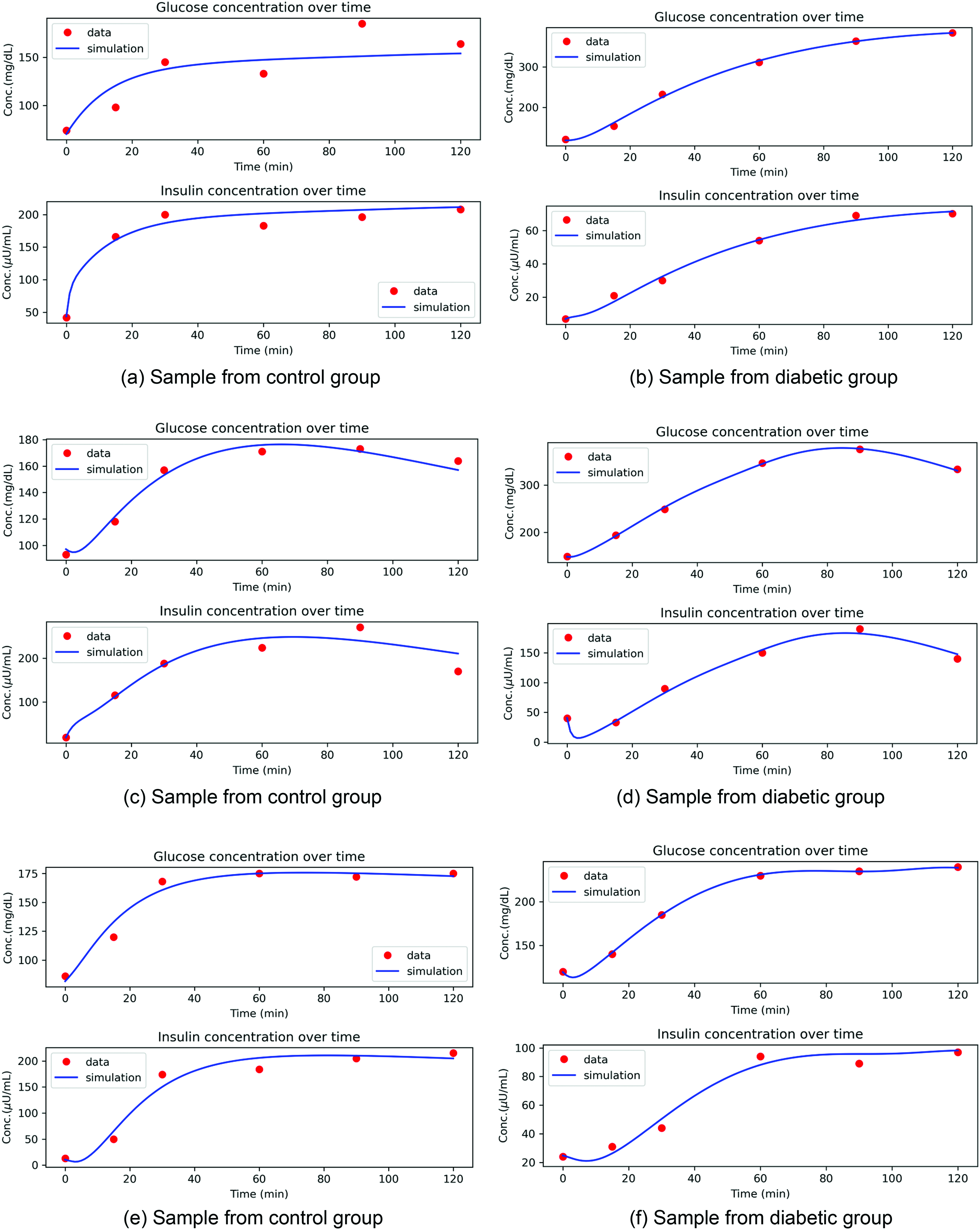
Sample simulation results for control and diabetic group. (a) Sample from control group; (b) sample from diabetic group; (c) sample from control group; (d) sample from diabetic group; (e) sample from control group; (f) sample from diabetic group.

FIG. 5.

Sample simulation results for obese and non-obese diabetic group. (a) Sample from obese diabetic group; (b) sample from non-obese diabetic group; (c) sample from obese diabetic group; (d) sample from non-obese diabetic group; (e) sample from obese diabetic group; (f) sample from non-obese diabetic group.

FIG. 6.

Box plots of parameters that are distinct for obese and non-obese diabetic subjects.

Table3.

Comparison of parameters in control and diabetic group with p-value, distribution, statistical test, and specifying distinct feature or not

Parameter	Control group	Diabetic group	p-Value	Distribution	Statistical test	Distinct feature
k_max (1/min)	0.0179	0.0269	0.000143	Lognormal	Independent t-test	Yes
k_min (1/min)	0.00137	0.00751	7.49E−27	Weibull	Mann–Whitney U test	Yes
k_abs (1/min)	0.0289	0.0208	0.0901	Lognormal	Independent t-test	No
p₁ (1/min)	0.0609	0.0208	2.45E−26	Weibull	Mann–Whitney U test	Yes
p₂ (1/min)	0.0016	0.0016	0.579	Weibull	Mann–Whitney U test	No
p₃ ((L/μmol)min⁻²)	1.50E−07	1.50E−07	0.618	Weibull	Mann–Whitney U test	No
p₄ (1/min)	0.154	0.863	5.61E−26	Weibull	Mann–Whitney U test	Yes
f (dimensionless)	0.756	0.891	0.000125	Beta	Mann–Whitney U test	Yes
G_b (μmol/L)	4.76E+03	7.30E+03	1.06E−12	Beta	Mann–Whitney U test	Yes
I_b (μmol/L)	2.22E−11	2.22E−11	0.232	Weibull	Mann–Whitney U test	No
G_T (μmol/L)	4.24E + 03	3.57E + 03	0.364	gamma (Γ)	Mann Whitney U test	No
γ (min⁻²)	2.80E−08	1.27E−08	2.15E−09	Weibull	Mann–Whitney U test	Yes

Table4.

Comparison of parameters in obese diabetic and non-obese diabetic groups with p-value, distribution, statistical test, and specifying distinct feature or not

Parameter	Obese diabetic (median)	Non-obese diabetic (median)	p-Value	Distribution	Statistical test	Distinct feature
k_max (1/min)	0.0166	0.0182	0.561	Gamma (Γ)	Mann–Whitney U test	No
k_min (1/min)	0.00563	0.00252	0.000925	t	Mann–Whitney U test	Yes
k_abs (1/min)	0.00722	0.00141	1.16E−06	Exponential	Mann–Whitney U test	Yes
p₁ (1/min)	0.0565	0.15	0.000141	Weibull	Mann–Whitney U test	Yes
p₂ (1/min)	0.00153	0.00808	0.451	Weibull	Mann–Whitney U test	No
p₃ ((L/μmol)min⁻²)	2.48E−07	5.97E−08	0.186	Weibull	Mann–Whitney U test	No
p₄ (1/min)	0.91	0.921	0.146	Weibull	Mann–Whitney U test	No
f (dimensionless)	0.826	0.784	0.0259	Weibull	Mann–Whitney U test	Yes
G_b (μmol/L)	7.31E + 03	5.04E + 03	0.0292	Beta	Mann–Whitney U test	Yes
I_b (μmol/L)	5.34E−12	5.01E−13	0.533	Beta	Mann–Whitney U test	No
G_T (μmol/L)	4.58E + 03	9.27E + 03	0.102	Gamma (Γ)	Mann–Whitney U test	No
γ (min⁻²)	1.65E−08	3.54E−09	0.134	Gamma (Γ)	Mann–Whitney U test	No

Distribution of parameters and statistical test

Understanding the distribution of each parameter is vital for selecting the right statistical test. The distribution of each parameter was examined to determine the appropriate statistical tests for comparing the control and diabetic groups (Dataset-1) and the obese and non-obese diabetic groups (Dataset-2). If the data do not follow a normal distribution, the Mann–Whitney U test (also known as the Wilcoxon rank-sum test) is used to compare two groups. It is a robust alternative to the t-test and does not require normality or equal variances. It is particularly useful if the sample size is small, and the data are ordinal or continuous. For instance, in the control and diabetic group, k_min follows the Weibull distribution (Table3), and a common non-normal distribution test, known as the Mann–Whitney U test, is used. Similarly, appropriate statistical tests are chosen based on parameter distribution, and the p-value is determined with significance level α = 0.05. The distribution followed and tests used for the control and diabetic group using Dataset-1 are shown in Table3, and the obese and non-obese diabetic groups using Dataset-2 are shown in Table4.

Discussion

Our results emphasize the difference in parameter values in different T2DM groups. From Table3, the control group differs from T2D groups based on parameters k_max, k_min, f, p₁, G_b, p₄, and γ. The model parameters conform with the previously published results for diabetic patients, which are described in detail in this section. The maximum and minimum amount of glucose emptying (k_max and k_min) for the diabetic group is higher. In support of this observation, it can be argued that rapid gastric emptying is frequent and important for diabetic complications.25 To improve the postprandial glycemic control in these patients, a slowing gastric emptying rationale may be considered. The fraction of intestinal absorption (f), which actually appears in plasma, is higher for the diabetic group. In patients with T2DM, an increase of the Sodium/GLucose coTransporter 1 (SGLT1) protein and its mRNA in the enterocytes of the small intestine were found, which is involved in increased glucose absorption through the apical membrane.26 The insulin-independent rate of glucose uptake (p₁), which also represents glucose effectiveness, is more in the control group than in the diabetic group. This may be attributed to insulin resistance among the diabetes group. The basal level of glucose (G_b) is higher in the diabetes group, which indicates pre-diabetes or diabetes, which is expected. As this parameter is less sensitive, the variation among subgroups is larger but less significant. Smaller changes in basal level of glucose do not change the model behavior. The decay rate for insulin (p₄) is significantly higher in the diabetic group. The excess insulin produced is rapidly attenuated due to acute induction of mitochondrial superoxide production.27 The rate of β-cells release of insulin (γ) after oral glucose intake is lower in the diabetic group. This may be due to a decrease in insulin sensitivity and secretion caused by a delay in glucose peak time.28

The analysis of data using the model for obese and non-obese indicated that the parametric range is different for the two groups. From Table4, it can be observed that the obese diabetic group differs from non-obese diabetic groups based on parameters k_min, k_abs, f, p₁, and G_b. The five estimated parameters are significant for obese and non-obese T2D groups. The minimum level of gastric emptying (k_min) is higher for obese, i.e., from that point, the emptying rate increases to k_max, not reducing any further. Obese subjects have a more rapid emptying rate for solids than non-obese subjects.29 The absorption rate in the intestine (k_abs) is higher for obese diabetics. The body surface area for obese subjects is larger, and therefore, the absorption rate increases. The insulin-independent glucose uptake rate (p₁) is higher for non-obese diabetics. This observation is associated with adiposity with declining glucose tolerance. During increased insulin resistance, this mechanism helps preserve glucose uptake.30 The fraction of intestinal absorption (f) is higher for the obese group. This has the same explanation for why k_abs is higher for the obese diabetic group. The basal glucose level (G_b) is higher for the obese diabetic group. These significant changes in parameter values for obese and non-obese indicate a higher risk of diabetes as it causes both insulin resistance and β-cell dysfunction.

The differences in obese and non-obese diabetes groups have to be discussed further as it is being considered as a novel category of diabetes. The degree of change and the direction of parameter values to increase or decrease diabetes risk is studied. The risk of T2D increases for an obese group with an increase in the value of parameter k_min as compared to the non-obese group. The insulin-independent rate of glucose uptake (p₁) is 2.6 times lower in the obese diabetic group, indicating a higher risk in obese diabetes. The absorption rate in the intestine (k_abs) in the obese group is five times higher compared to the non-obese group, indicating higher levels of glucose in the non-obese diabetes group. This is also supported by a higher fraction of intestinal absorption (f). The higher basal glucose level (G_b) in the obese diabetic group indicates more insulin resistance. From the comparison, it can also be concluded that the obese group is more insulin-resistant than the non-obese group.

Some of the limitations and biases of the study are discussed. The OMM assumes linear relationships between glucose and insulin concentrations, which may not always hold true. The model assumes insulin acts only on glucose uptake in peripheral tissues, ignoring potential effects on glucose production and other metabolic processes. The model does not account for feedback mechanisms, such as the effects of glucose on insulin secretion or the regulation of glucose production by the liver. The model assumes steady-state conditions, whereas in reality, glucose and insulin concentrations can fluctuate significantly over time. The model simplifies the complex physiological processes involved in glucose regulation, which may lead to oversimplification or omission of important mechanisms. Some of the biases in the dataset may include possibility of measurement errors (e.g., blood glucose levels). Patients selected for the study may not be representative of the larger population (e.g., age, gender, and ethnicity) and may have different characteristics than those who did not participate in the study. The variables not accounted for in the study may influence the results (e.g., socioeconomic status and access to healthcare). The study population may not be representative of the target population (e.g., age range and comorbidities) and may not generalize well to other populations.

The present study has some specific limitations with confounding variables. First, a large number of samples across different ethnicities needs to be analyzed for more generalized and clinically relevant conclusions. Second, the IG axis is modulated by multiple factors, including certain adipokines such as adiponectin, resistin, visfatin, adipsin, and other hormones such as glucagon and GLP-1. Our study, albeit a preliminary one, might have important clinical implications, particularly in designing patient-specific tailored therapy. As non-obese subtypes of T2DM have impaired insulin production, the therapeutic guidelines for these patients would need a revisit. Insulin sensitizers such as metformin and thiazolidinediones may not serve as first-line drugs for these patients. Also, obese patients with increased intestinal glucose absorption may benefit from medications that alter glucose absorption, one being alpha-glucosidase inhibitors.

Conclusion

In this study, we adapted a published model to determine the significant changes in parameter values for healthy and diabetic groups and further among obese and non-obese diabetes groups. This is the first attempt to use the OMM to corelate the parameters for different diabetic groups using OGTT data. The parameter values that were sensitive among groups were corelated to the known biological findings. The obese diabetic group is more insulin resistant, whereas the non-obese diabetic group is less insulin resistant. As non-obese T2DM is becoming more recognized, a model to identify the differences in insulin secretion and glucose absorption among these phenotypes is important. More relevant studies can be conducted using this model estimation, which paves the way to precision therapy in T2DM.

Declaration of Competing Interest: The authors declare that there are no conflicts of interest.

Authorship Contribution: MRA: Conceptualization, Formal analysis, Methodology, Validation, Writing – original draft; DG: Conceptualization, Methodology, Supervision; CM: Formal analysis, Supervision, Writing – review & editing; KVV: Data curation, Supervision; JS: Data curation, Investigation, Writing – review & editing; PC: Supervision, Writing – review & editing; SKM: Data curation.

Disclaimer

This paper has been previously submitted to medRxiv (https://www.medrxiv.org/) and is available online at doi: 10.1101/2024.04.06.24305200.

Footnotes

Acknowledgments

The authors gratefully thank the associates of KV Venkatesh for collecting the insulin-glucose time series data. MRA acknowledges funding from MoE, Government of India, under Award No. R/F.II/2//19/CS/92P03.

Highlights

References

U.S. Department of Health and Human Services. Diabetes & prediabetes tests. 2020. Available at https://www.niddk.nih.gov/health-information/professionals/clinical-tools-patient-management/diabetes/diabetes-prediabetes?dkrd=hisce0124.

Burkart

, Huber

MF.

A survey on the explainability of supervised machine learning. J Artif Intell Res. 2021; 70: 245–317. DOI: 10.1613/jair.1.12228.

Karim

, Beyan

, Zappa

, et al. Deep learning-based clustering approaches for bioinformatics. Brief Bioinform. 2020; 22(1): 393–415. DOI: 10.1093/bib/bbz170.

, Ma

, Shende

, et al. Using machine learning of clinical data to diagnose COVID-19: A systematic review and meta-analysis. BMC Med Inform Decis Mak. 2020; 20(1). DOI: 10.1186/s12911-020-01266z.

Ambigavathi

, Sridharan

Analysis of clustering algorithms in machine learning for healthcare data. Commun Comput Inform Sci. 2020; 117–128. DOI: 10.1007/978-981-15-6634-9_12.

Aravindakshan

, Maity

, Paul

, et al. Distinct pathoclinical clusters among patients with uncontrolled type 2 diabetes: Results from a prospective study in rural India. BMJ Open Diabetes Res Care. 2022; 10(1): e002654. DOI: 10.1136/bmjdrc-2021-002654.

Bergman

RN.

The minimal model of glucose regulation: A biography. Adv Exp Med Biol. 2003; 1–19. Available at https://pubmed.ncbi.nlm.nih.gov/14995025/.

Bolie

VW.

Coefficients of normal blood glucose regulation. J Appl Physiol. 1961; 16(5): 783–788. DOI: 10.1152/jappl.1961.16.5.783.

Sturis

, Polonsky

, Mosekilde

, et al. Computer model for mechanisms underlying ultradian oscillations of insulin and glucose. Am J Physiol Endocrinol Metabol. 1991; 260(5): E801–E809. DOI: 10.1152/ajpendo.1991.260.5.e801.

10.

Hovorka

, Canonico

, Chassin

, et al. Nonlinear model predictive control of glucose concentration in subjects with type 1 diabetes. Physiol Meas. 2004; 25(4): 905–920. DOI: 10.1088/0967-3334/25/4/010.

11.

Dalla Man

, Caumo

, Cobelli

The oral glucose minimal model: Estimation of insulin sensitivity from a meal test. IEEE Trans Biomed Eng. 2002; 49(5): 419–429. DOI: 10.1109/10.995680.

12.

Lehmann

, Deutsch

A physiological model of glucose-insulin interaction in type 1 diabetes mellitus. J Biomed Eng. 1992; 14(3): 235–242. DOI: 10.1016/0141-5425(92)90058-s.

13.

Elashoff

, Reedy

, Meyer

JH.

Analysis of gastric emptying data. Gastroenterology. 1982; 83(6): 1306–1312. Available at https://pubmed.ncbi.nlm.nih.gov/7129034/.

14.

Man

, Camilleri

, Cobelli

A system model of oral glucose absorption: Validation on gold standard data. IEEE Trans Biomed Eng. 2006; 53(12): 2472–2478. DOI: 10.1109/tbme.2006.883792.

15.

Misra

Ethnic-specific criteria for classification of body mass index: A perspective for Asian Indians and American Diabetes Association position statement. Diabetes Technol Therap. 2015; 17(9): 667–671. DOI: 10.1089/dia.2015.0007.

16.

Man

, Cobelli

Glucose modelling. Model. Method. Physiol. Med., 2014; 355–379. DOI: 10.1016/b978-0-12-411557-6.00016-1.

17.

Wentworth

, Smith

, Banks

HT.

Parameter selection and verification techniques based on global sensitivity analysis illustrated for an HIV model. SIAM/ASA J Uncertain Quantif. 2016; 4(1): 266–297. DOI: 10.1137/15m1008245.

18.

Chu

, Hahn

Parameter set selection for estimation of nonlinear dynamic systems. AIChE J. 2007; 53(11): 2858–2870.

19.

Walter

, Pronzato

Qualitative and quantitative experiment design for phenomenological models—A survey. Automatica. 1990; 26(2): 195–213.

20.

Schittkowski

Parameter estimation in dynamic systems. Yang

, Mees

, Fisher

, Jennings

(eds), Progress in optimization. Applied optimization, Vol 39. Springer: Boston, MA; 2000. DOI: 10.1007/978-1-4613-0301-5_13.

21.

Guedj

, Thiébaut

, Commenges

Maximum likelihood estimation in dynamical models of HIV. Biometrics. 2007; 63(4): 1198–1206. DOI: 10.1111/j.1541-0420.2007.00812.x.

22.

Singer

, Nelder

Nelder-Mead algorithm. Scholarpedia. 2009; 4(7): 2928.

23.

Brun

, Reichert

, Künsch

HR.

Practical identifiability analysis of large environmental simulation models. Water Resour Res. 2001; 37(4): 1015–1030. DOI: 10.1029/2000WR900350.

24.

Virtanen

, Gommers

, Oliphant

, et al. SciPy 1.0: Fundamental algorithms for scientific computing in Python. Nat Methods. 2020; 17(3): 261–272.

25.

Goyal

, Cristofaro

, Sullivan

MP.

Rapid gastric emptying in diabetes mellitus: Pathophysiology and clinical importance. J Diabetes Complications. 2019; 33(11): 107414. DOI: 10.1016/j.jdiacomp.2019.107414.

26.

Gromova

, Fetissov

, Gruzdkov

AA.

Mechanisms of glucose absorption in the small intestine in health and metabolic diseases and their role in appetite regulation. Nutrients. 2021; 13(7): 2474. DOI: 10.3390/nu13072474.

27.

Hoehn

, Salmon

, Hohnen-Behrens

, et al. Insulin resistance is a cellular antioxidant defense mechanism. Proc Natl Acad Sci U S A. 2009; 106(42): 17787–17792. DOI: 10.1073/pnas.0902380106.

28.

Wang

, Zhao

, Zhou

, et al. Delay in glucose peak time during the oral glucose tolerance test as an indicator of insulin resistance and insulin secretion in type 2 diabetes patients. J Diabetes Investig. 2018; 9(6): 1288–1295. DOI: 10.1111/jdi.12834.

29.

Wright

, Krinsky

, Fleeman

, et al. Gastric emptying and obesity. Gastroenterology. 1983; 84(4): 747–751. DOI: 10.1016/0016-5085(83)90141-5.

30.

Jumpertz

, Thearle

, Bunt

, etal. Assessment of non-insulin-mediated glucose uptake: Association with body fat and glycemic status. Metabolism. 2010; 59(10): 1396–1401. DOI: 10.1016/j.metabol.2010.01.006.

Parameter Estimation for the Oral Minimal Model and Parameter Distinctions Between Obese and Non-Obese Type 2 Diabetes

Abstract

Abstract

Background:

Method:

Result:

Conclusion:

Introduction

Model Under Consideration

Theory

Parameter sensitivity analysis methods

Parameter estimation methods

Methodology

Datasets used for parameter estimation

Parameter sensitivity indices

Parameter estimation

Results

Sensitivity indicators

Results of parameter estimation

Distribution of parameters and statistical test

Discussion

Conclusion

Disclaimer

Footnotes

Acknowledgments

Highlights

References