Missing values in complex biological data sets have significant impacts on our ability to correctly detect and quantify interactions in biological systems and to infer relationships accurately. In this article, we propose a useful metaphor to show that information theory measures, such as mutual information and interaction information, can be employed directly for evaluating multivariable dependencies even if data contain some missing values. The metaphor is that of thinking of variable dependencies as information channels between and among variables. In this view, missing data can be thought of as noise that reduces the channel capacity in predictable ways. We extract the available information in the data even if there are missing values and use the notion of channel capacity to assess the reliability of the result. This avoids the common practice—in the absence of prior knowledge of random imputation—of eliminating samples entirely, thus losing the information they can provide. We show how this reliability function can be implemented for pairs of variables, and generalize it for an arbitrary number of variables. Illustrations of the reliability functions for several cases are provided using simulated data.
1. Introduction
Biological systems are composed of a large number of components that interact, constitute, transmit, and exchange information in a complex manner (Galas et al., 2014). The wide range of heterogeneous data on biological systems that are increasingly available presents both great opportunities and challenges in the effort to reconstruct the underlying dependency structure of the systems, and hence biological mechanisms, from data characterizing biological variables. The relevant probability distributions of various biological data types are generally not known (Weng et al., 1999; Adami et al., 2000). Moreover, most data obtained from experiments are incomplete for various reasons. For example, the human genomic data of the sequences of single nucleotide polymorphisms (SNPs) often have significant number of missing values (Hutter and Zaffalon, 2005; Su et al., 2005; Hudson et al., 2014). Typically, missing SNP data range from ∼10% to 20% in human genome data sets (Daly et al., 2001; Patil et al., 2001). Medical data, and particularly patient and subject self-reported information, are notoriously fraught with missing data points. These and other forms of missing values in data sets have a significant impact on our ability to correctly detect and quantify interactions in biological systems.
Inference methods based on statistical approaches such as expectation–maximization algorithms are commonly used for inferring missing data. Furthermore, these methods typically use specific probability distributions as priors, for example, when imputing missing SNP data (Stephens and Scheet, 2005). There have been many approaches to imputation and model-free inference in the analysis of biological data.
Information theory-based methods have been increasingly successful in searching for interactions by detecting and reconstructing the dependency structure from biological data, due, in part, to their inherently model-free nature (Galas et al., 2010; Sakhanenko and Galas, 2011, 2015; Sakhanenko et al., 2017). However, these methods also suffer from the missing data problem, and can thereby encounter significant difficulty in drawing conclusions and in estimating statistical significance of detected interactions. Some methods attempt to complement incompleteness of data using posterior distributions, which are obtained in a Bayesian framework by a second-order Dirichlet prior distribution (Hutter and Zaffalon, 2005). Other methods combine information theory measures with algorithms from machine learning, for example, Greedy and Nearest Neighbor algorithms have been used for feature selection from incomplete data (Doquire and Verleysen, 2011; Qian and Shu, 2015). However, when we have little or no information about prior distributions, as is common for biological data (e.g., RNA levels, gene expression data, protein levels and patterns of phenotypes, and medical record data), these inference methods all fail.
Systematic and assumption-free methods of extracting accurate information, including dependencies among variables, and assessing its reliability from data that are incomplete, are needed. In this article, we suggest a useful metaphor for which information theory measures, such as mutual information and interaction information, can be employed directly for evaluating multivariable dependencies, even if the data have some missing values. The metaphor we propose is that of thinking of variable dependencies as information channels. In this view, missing data can be thought of as reducing the channel capacity in predictable ways. We extract the available information in the data even when it has missing values and use the notion of channel capacity to assess its reliability. This avoids the common practice, in the absence of prior knowledge for informed imputation, of eliminating samples entirely and, therefore, losing the information they can provide. Since this can be done without making any assumption about prior probability distributions, it can be universally applied. Another common practice of adding random values where missing values occur has the effect of changing the significance of the result in unknown ways. The reliability function proposed here can provide a precise estimate of its reliability.
Since the missing values are viewed as a reduction in the channel capacity, a specific “reliability function” can be derived from information theory to quantitatively describe these channel capacities. This reliability function then expresses the maximum amount of information about a given dependence (including multiple variable dependencies) we could possibly find given the level of missing data.
In the next section, we summarize the information theory-based analysis context relevant to our formulation, then in the following section we discuss the missing values problem and the communications channel idea in more detail. Finally, in the following sections, we define and characterize a reliability function for both pairwise variable dependencies and multivariable problems.
2. Dependence Detection Using Information Theory
The context of this work on the problem of missing data comes from the search for multivariable dependencies in biological data, using measures of dependence from information theory (McGill, 1954; Sakhanenko and Galas, 2015; Sakhanenko et al., 2017). In this section, we briefly review the basic relationships that are used in this analysis and will be shown to lead to the derivation of the reliability functions.
Mutual information is perhaps the most well-known measure of pairwise information, which measures the amount of information about one variable embodied in the knowledge of another (Khinchin, 1957). It is defined as
\documentclass{aastex}\usepackage{amsbsy}\usepackage{amsfonts}\usepackage{amssymb}\usepackage{bm}\usepackage{mathrsfs}\usepackage{pifont}\usepackage{stmaryrd}\usepackage{textcomp}\usepackage{portland, xspace}\usepackage{amsmath, amsxtra}\usepackage{upgreek}\pagestyle{empty}\DeclareMathSizes{10}{9}{7}{6}\begin{document}
\begin{align*}
I \left( {{X_1} , {X_2}} \right) = H \left( {{X_1}} \right) + H \left( {{X_2}} \right) - H \left( {{X_1} , {X_2}} \right) , \tag{1}
\end{align*}
\end{document}
where H(Xi) is an entropy of Xi and H(X1,X2) is a joint entropy of variables X1 and X2. Mutual information is equal to Kullback–Leibler divergence of the joint-to-single probability distributions of two variables (Galas et al., 2010; Sakhanenko and Galas, 2011, 2015), a measure of the deviation of the pair probability distribution from independence.
A generalization of mutual information to more than two variables, called interaction information, was proposed in the 1950s (McGill, 1954). Similar to mutual information, it is a symmetric function that is defined in terms of joint entropies. For three variables, the interaction information is
\documentclass{aastex}\usepackage{amsbsy}\usepackage{amsfonts}\usepackage{amssymb}\usepackage{bm}\usepackage{mathrsfs}\usepackage{pifont}\usepackage{stmaryrd}\usepackage{textcomp}\usepackage{portland, xspace}\usepackage{amsmath, amsxtra}\usepackage{upgreek}\pagestyle{empty}\DeclareMathSizes{10}{9}{7}{6}\begin{document}
\begin{align*}
\begin{split} I \left( {{X_1} , {X_2} , {X_3}} \right) & = H \left( {{X_1}} \right) + H \left( {{X_2}} \right) + H \left( {{X_3}} \right) \\ &\quad - H \left( {{X_1} , {X_2}} \right) - H \left( {{X_1} , {X_3}} \right) - H \left( {{X_2} , {X_3}} \right) + H \left( {{X_1} , {X_2} , {X_3}} \right). \\ \end{split}
\tag{2}
\end{align*}
\end{document}
This definition can also be rewritten as a recursive relation, arbitrarily choosing X3 as a “target” (conditional) variable:
\documentclass{aastex}\usepackage{amsbsy}\usepackage{amsfonts}\usepackage{amssymb}\usepackage{bm}\usepackage{mathrsfs}\usepackage{pifont}\usepackage{stmaryrd}\usepackage{textcomp}\usepackage{portland, xspace}\usepackage{amsmath, amsxtra}\usepackage{upgreek}\pagestyle{empty}\DeclareMathSizes{10}{9}{7}{6}\begin{document}
\begin{align*}
I \left( {{X_1} , {X_2} , {X_3}} \right) = I \left( {{X_1} , {X_2}} \right) - I \left( {{X_1} , {X_2} \vert {X_3}} \right) , \tag{3}
\end{align*}
\end{document}
where \documentclass{aastex}\usepackage{amsbsy}\usepackage{amsfonts}\usepackage{amssymb}\usepackage{bm}\usepackage{mathrsfs}\usepackage{pifont}\usepackage{stmaryrd}\usepackage{textcomp}\usepackage{portland, xspace}\usepackage{amsmath, amsxtra}\usepackage{upgreek}\pagestyle{empty}\DeclareMathSizes{10}{9}{7}{6}\begin{document}
$$I ( {X_1} , {X_2} \vert {X_3} )$$
\end{document} is the conditional mutual information for a given X3. Equation (3) shows the important point that if the additional variable X3 is independent of the other two, the interaction information becomes 0.
For a set of n variables \documentclass{aastex}\usepackage{amsbsy}\usepackage{amsfonts}\usepackage{amssymb}\usepackage{bm}\usepackage{mathrsfs}\usepackage{pifont}\usepackage{stmaryrd}\usepackage{textcomp}\usepackage{portland, xspace}\usepackage{amsmath, amsxtra}\usepackage{upgreek}\pagestyle{empty}\DeclareMathSizes{10}{9}{7}{6}\begin{document}
$${V_n} = \{ {X_1} , {X_2} \ldots , {X_n} \} $$
\end{document}, the interaction information is defined as sums of joint entropies
\documentclass{aastex}\usepackage{amsbsy}\usepackage{amsfonts}\usepackage{amssymb}\usepackage{bm}\usepackage{mathrsfs}\usepackage{pifont}\usepackage{stmaryrd}\usepackage{textcomp}\usepackage{portland, xspace}\usepackage{amsmath, amsxtra}\usepackage{upgreek}\pagestyle{empty}\DeclareMathSizes{10}{9}{7}{6}\begin{document}
\begin{align*}
I ( {V_n} ) = \sum \nolimits_{ \tau \subseteq {V_ \nu }} {{{ ( - 1 ) }^{ \vert \tau \vert + 1}}H ( \tau ) } , \tag{4}
\end{align*}
\end{document}
where the sum is over all possible τ, subsets of Vn, and |τ| is the cardinality of the subset, τ.
The differential interaction information is defined as the change in the interaction information among sets by the addition of one variable:
\documentclass{aastex}\usepackage{amsbsy}\usepackage{amsfonts}\usepackage{amssymb}\usepackage{bm}\usepackage{mathrsfs}\usepackage{pifont}\usepackage{stmaryrd}\usepackage{textcomp}\usepackage{portland, xspace}\usepackage{amsmath, amsxtra}\usepackage{upgreek}\pagestyle{empty}\DeclareMathSizes{10}{9}{7}{6}\begin{document}
\begin{align*}
\Delta ( {X_i} , {V_n} ) = I ( {V_n} ) - I ( {V_n} \backslash \{ {X_i} \} ) = - I ( {V_n} \backslash \{ {X_i} \} \vert {X_i} ) , \tag{5}
\end{align*}
\end{document}
where Vn\{Xi} is the set Vn without variable Xi. As shown by the second equality, the differential interaction information is equivalent to the conditional interaction information. It is easy to see that if the target variable Xi is independent from any of the variables in the set Vn\{Xi}, then the differential interaction information is 0. The differential interaction information is thus a measure of dependence in this way.
These information theory-based measures have several advantages that make them useful for dependency detection. First, these measures are model-free in that they make no assumptions about the nature of the underlying function of the dependence or about the probability distributions of the variables. Since the information required for detection of dependence is less than that required for defining the functional form of dependence, detection with these measures is more resistant to undersampling. These measures have been applied successfully to detect and quantify both pairwise and multivariable dependencies in biological data (Galas et al., 2010, 2014; Sakhanenko and Galas, 2015; Sakhanenko et al., 2017).
3. The Problem of Missing Data
A number of factors can affect the calculation of dependency measures, such as noise of several kinds, missing data, and undersampling. In this article, we focus only on the problem of missing data. In this section, we describe the problem, show how it can affect accuracy, and how missing values can be handled using information theory methods.
As mentioned in Section 1, there are various approaches to handling missing data. Let us distinguish three main types:
The samples with missing data are omitted individually for the calculation of each entropy term on an as-needed basis.
The samples with many missing values are removed at the outset and not used for the calculation at all.
The missing values are inferred or filled with random values.
Consider a simple toy data set with 3 variables and 10 samples:
1
2
3
4
5
6
7
8
9
10
X
0
1
1
0
0
0
1
0
0
0
Y
0
1
0
?
1
1
1
0
1
0
Z
0
0
1
0
0
0
0
0
0
0
In our example, variable Y has a missing value in sample 4, denoted by the symbol “?”
Using approach (i) we simply skip the missing values during the entropy calculation involving Y. In this article, we calculate entropies using the “naive” or “point” form based on probabilities estimated as frequencies. Table 1(a) shows single and joint entropies as well as mutual information.
Entropies and Mutual Information Calculated Using Three Approaches to Handling Missing Data
X
Y
Z
X
Y
Z
X
Y
Z
X
Y
Z
X
0.881
−0.019
0.194
0.918
0.018
0.197
0.881
0.035
0.194
0.881
0.006
0.194
Y
1.891
0.991
0.108
1.891
0.991
0.143
1.846
1.0
0.108
1.846
0.971
0.145
Z
1.157
1.352
0.469
1.224
1.352
0.503
1.157
1.361
0.469
1.157
1.296
0.469
(a)
(b)
(c)
(d)
Tables (a) and (b) correspond to approaches (i) and (ii). Tables (c) and (d) correspond to approach (iii), where the missing value is replaced with either 0 or 1. The diagonal elements of each table correspond to single entropies, the elements of the bottom half correspond to the joint entropies, and the elements of the top half (highlighted) correspond to mutual information.
Note that the mutual information calculated between X and Y is negative due to the single missing value, which, of course, violates the non-negativity property of mutual information.
We could use approach (ii) instead and completely eliminate the samples with missing values from the calculations. Recomputing Table 1(a) in this case results in the values in Table 1(b). This resolves the issue of negative mutual information, but discards information in the process. Notice that the mutual information values go up in a nonuniform manner compared with the previous case, for example, while I(X,Z) goes up by 2%, I(Y,Z) goes up by 32%. Such induced fluctuations are typical when there is insufficient data, so discarding data must be avoided wherever possible. Another version of approach (ii) is to optimize the selection of samples/variables by minimizing the amount of information deleted, allowing some missing values to remain in the data. This approach still discards information from the data, although not as much as in the original approach.
The alternative approach (iii) is to fill in the missing values with either some sort of inferred, or partially inferred values, or with random values. Table 1(c, d) shows the corresponding entropies and mutual information for the cases when the missing value is filled in with either 0 or 1. This approach also resolves the issue of negative mutual information and preserves all the information in the samples; however, it can introduce bias and/or noise into the data, causing spurious effects, for example, I(X,Z) goes from 0.108 when the missing value is filled in with 0 to 0.1445 when the missing value is filled in with 1, a 34% change from a single imputed missing value. Of course, this issue is exacerbated here by the small amount of data, but it clearly illustrates that filling in the missing data can bias the results. One way to reduce this bias is to infer missing values by applying some statistical inference approaches [expectation–maximization, Gibbs sampling (Su et al., 2005), etc.], which make assumptions about probability distributions of the data, using Dirichlet priors or the approximate coalescent prior. Although these approaches can be useful in imputing SNP data, they are not applicable for most other biological data sets where the distributions are unknown (Doan et al., 2016).
The example mentioned shows that there is no single best approach of handling the missing values—every approach has its limitations that can be quite detrimental in the downstream dependency analysis using information theory. Volatile information scores that can be large enough to be significantly misinterpreted as a real signal in the data, information loss, and biased computation are all problems we face when dealing with missing values. The missing values problem is thus an important practical problem when searching for and quantitating multivariable dependencies. Note that although we used mutual information to illustrate the challenges of handling missing data, same issues arise when using other more general information measures, such as interaction information or the Delta measure (differential interaction information).
In the next section, we introduce the idea that missing data are like a noisy communications channel between the variables concerned. This notion leads us to the idea of the channel capacity between dependent variables. We can calculate the channel capacity in such channels that have been degraded by the occurrence of missing data by extending the metaphor that missing data are noise and using the usual communications relations. We then define the reliability function as the quantitative level that the channel capacity has been degraded by missing data points.
4. The Reliability Function
4.1. Binary symmetric channels
The binary channel is a most basic model of a communication system. Consider a channel between binary variables X and Y, which specify an input and an output, containing a source of errors or noise (Shannon, 1949, 2001; Verdu and Han, 1994; Ashikhmin et al., 2000; Tishby et al., 2000; Slonim, 2002; Reyes-Valdes and Williams, 2005; Cover and Thomas, 2012). Let e represent the probability of a communication error in this binary input–output channel. The conditional probability p(Y|X) of an output given an input in the presence of errors is then defined in Table 2.
Conditional Probability Table for a Pairwise Case, \documentclass{aastex}\usepackage{amsbsy}\usepackage{amsfonts}\usepackage{amssymb}\usepackage{bm}\usepackage{mathrsfs}\usepackage{pifont}\usepackage{stmaryrd}\usepackage{textcomp}\usepackage{portland, xspace}\usepackage{amsmath, amsxtra}\usepackage{upgreek}\pagestyle{empty}\DeclareMathSizes{10}{9}{7}{6}\begin{document}
$$X \to Y$$
\end{document}
X = 0
X = 1
\documentclass{aastex}\usepackage{amsbsy}\usepackage{amsfonts}\usepackage{amssymb}\usepackage{bm}\usepackage{mathrsfs}\usepackage{pifont}\usepackage{stmaryrd}\usepackage{textcomp}\usepackage{portland, xspace}\usepackage{amsmath, amsxtra}\usepackage{upgreek}\pagestyle{empty}\DeclareMathSizes{10}{9}{7}{6}\begin{document}
$$p \, ( Y = 0 \vert X )$$
\end{document}
1-e
e
\documentclass{aastex}\usepackage{amsbsy}\usepackage{amsfonts}\usepackage{amssymb}\usepackage{bm}\usepackage{mathrsfs}\usepackage{pifont}\usepackage{stmaryrd}\usepackage{textcomp}\usepackage{portland, xspace}\usepackage{amsmath, amsxtra}\usepackage{upgreek}\pagestyle{empty}\DeclareMathSizes{10}{9}{7}{6}\begin{document}
$$p \, ( Y = 1 \vert X )$$
\end{document}
e
1-e
The channel is symmetric in our case since each of the variables has information about the other. If X and Y are the input and the output of a communication channel governed by the conditional probability defined in Table 2, then the channel's mutual information between X and Y is calculated as
\documentclass{aastex}\usepackage{amsbsy}\usepackage{amsfonts}\usepackage{amssymb}\usepackage{bm}\usepackage{mathrsfs}\usepackage{pifont}\usepackage{stmaryrd}\usepackage{textcomp}\usepackage{portland, xspace}\usepackage{amsmath, amsxtra}\usepackage{upgreek}\pagestyle{empty}\DeclareMathSizes{10}{9}{7}{6}\begin{document}
\begin{align*}
\begin{split} I^{ch} ( X , Y ) & = - \mathop \sum \limits_{x} p ( x ) \log [ p ( x ) ] - \mathop \sum \limits_y p ( y ) \log [ p ( y ) ] \\ &\quad + \mathop \sum \limits_x \mathop \sum \limits_{y} p ( x , y ) \log [ p ( x , y ) ] \\ & = - \mathop \sum \limits_{y} \left[ \mathop \sum \limits_{x} p ( y \vert x ) p ( x ) \right] \log \left[ \mathop \sum \limits_{x} p ( y \vert x ) p ( x ) \right]\\ & \quad + \mathop \sum \limits_x \mathop \sum \limits_y p ( y \vert x ) p ( x ) \log [ p ( y \vert x ) ] \\ & = ( 1 - e ) {p_1} ( \log [ 1 - e ] - \log [ ( 1 - e ) {p_1} + e{p_2} ] ) \\ & \quad + e{p_1} ( \log [ e ] - \log [ e{p_1} + ( 1 - e ) {p_2} ] ) \\ & \quad + e{p_2} ( \log [ e ] - \log [ ( 1 - e ) {p_1} + e{p_2} ] ) \\ & \quad + ( 1 - e ) {p_2} ( \log [ 1 - e ] - \log [ e{p_1} + ( 1 - e ) {p_2} ] , \end{split}
\tag{6}
\end{align*}
\end{document}
where p1 = p(X = 0) and p2 = p(X = 1), so p1 + p2 = 1, and p(x) is a shorthand for p(X = x).
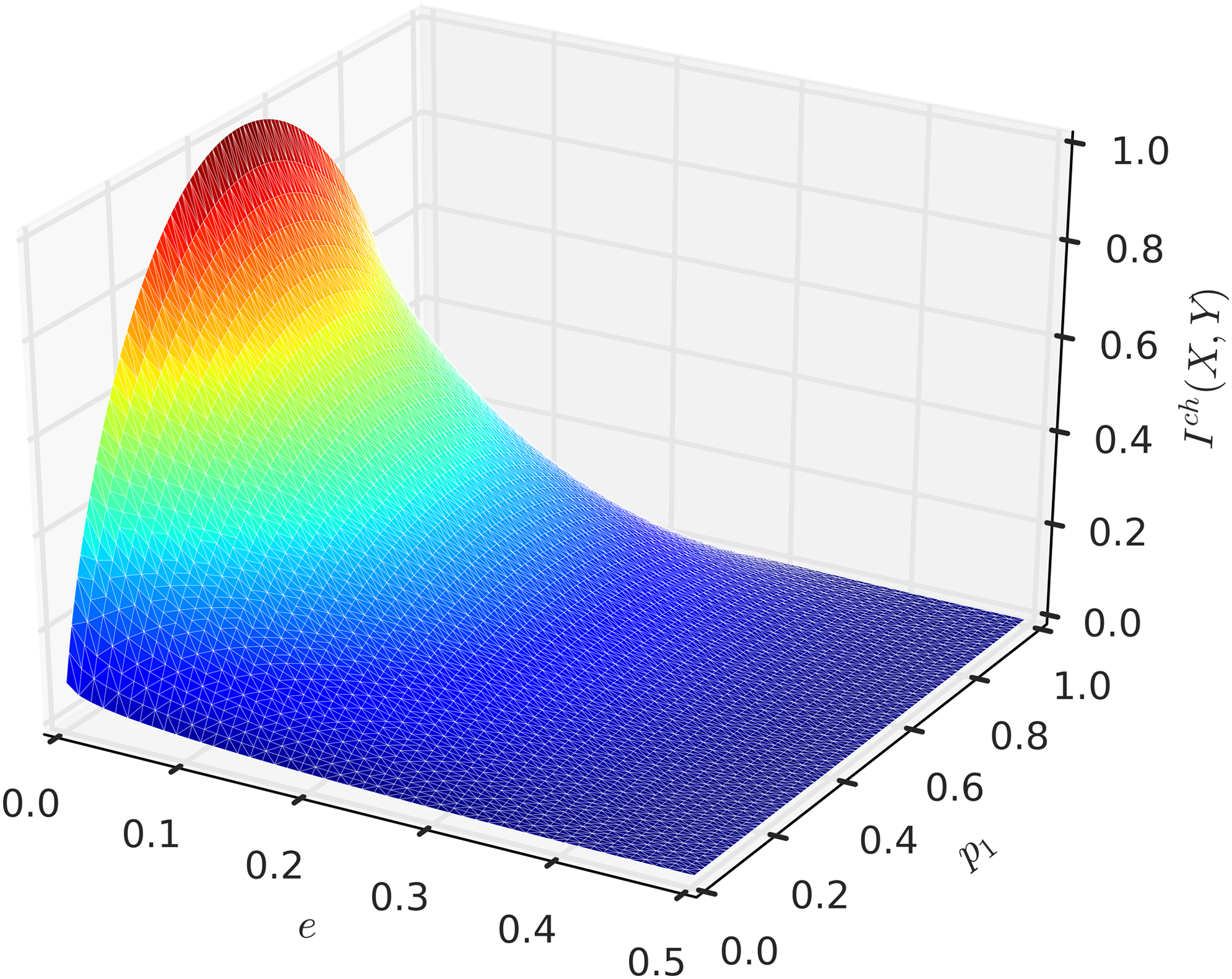
Larger values of Ich(X,Y) correspond to more accurate communication through the channel. In contrast, when the error increases to e = 1/2, then I(X,Y) is 0, indicating that it is impossible to transmit any information through this channel. According to the Shannon–Hartley theorem (Cover and Thomas, 2012) for any given level of noise e, Ich(X,Y) is maximized when the probability distribution is uniform, that is when p1 = p2 = 1/2, and it is called the channel capacity. The mutual information, Ich(X,Y), is a symmetric downward-convex function (Fig. 1). Therefore, Ich(X,Y) is maximal with respect to e when e is either 0 or 1, and this maximum, in terms of p1 and p2, is
\documentclass{aastex}\usepackage{amsbsy}\usepackage{amsfonts}\usepackage{amssymb}\usepackage{bm}\usepackage{mathrsfs}\usepackage{pifont}\usepackage{stmaryrd}\usepackage{textcomp}\usepackage{portland, xspace}\usepackage{amsmath, amsxtra}\usepackage{upgreek}\pagestyle{empty}\DeclareMathSizes{10}{9}{7}{6}\begin{document}
\begin{align*}
I_{max}^{ch} ( X , Y ) = - {p_1} \log {p_1} - {p_2} \log {p_2}. \tag{7}
\end{align*}
\end{document}
Mutual information of the communication channel \documentclass{aastex}\usepackage{amsbsy}\usepackage{amsfonts}\usepackage{amssymb}\usepackage{bm}\usepackage{mathrsfs}\usepackage{pifont}\usepackage{stmaryrd}\usepackage{textcomp}\usepackage{portland, xspace}\usepackage{amsmath, amsxtra}\usepackage{upgreek}\pagestyle{empty}\DeclareMathSizes{10}{9}{7}{6}\begin{document}
$${I^{ch}} ( X , Y )$$
\end{document} as a function of e and p1. The range of the error rate is limited to 0 < e < 0.5. When e = 0.5, \documentclass{aastex}\usepackage{amsbsy}\usepackage{amsfonts}\usepackage{amssymb}\usepackage{bm}\usepackage{mathrsfs}\usepackage{pifont}\usepackage{stmaryrd}\usepackage{textcomp}\usepackage{portland, xspace}\usepackage{amsmath, amsxtra}\usepackage{upgreek}\pagestyle{empty}\DeclareMathSizes{10}{9}{7}{6}\begin{document}
$${I^{ch}} ( X , Y )$$
\end{document} reaches 0.
Keep in mind that when e is 1, the information is fully restored, but the alphabet is simply inverted.
4.2. Reliability function in the pairwise case
We now use the idea of a communication channel to specifically define a reliability function that measures how much the missing data erode the mutual information. Given a pair of variables V1 and V2 representing biological measurements (SNPs, quantitative traits, gene expression levels, etc.), we want to know how much the missing data affect I(V1,V2). Since we view V1 and V2 as an input and output of a noisy binary symmetric transmission channel, where missing values are errors in transmission, we view data samples as packets of bits being transmitted from V1 to V2. If all samples have defined values for both variables V1 and V2 (or alternatively, both values are missing for some samples), then we interpret the channel as noise free, namely there is no error in the information transmission between V1 and V2. In contrast, if a sample has a defined value for V1 but not for V2, or vice versa, it is interpreted as an error in the information transmission between V1 and V2, and the overall noise is determined by the number of samples for which there are missing values. The model is embodied in this mapping φ:
\documentclass{aastex}\usepackage{amsbsy}\usepackage{amsfonts}\usepackage{amssymb}\usepackage{bm}\usepackage{mathrsfs}\usepackage{pifont}\usepackage{stmaryrd}\usepackage{textcomp}\usepackage{portland, xspace}\usepackage{amsmath, amsxtra}\usepackage{upgreek}\pagestyle{empty}\DeclareMathSizes{10}{9}{7}{6}\begin{document}
\begin{align*}
\varphi ( V ) = \left\{ { \begin{matrix} {1 , } \hfill & {{ \rm{if \ the \ value \ of }}\ V \ { \rm{ is \ missing}}} \hfill \\ {0 , } \hfill & {{ \rm{otherwise}}} \hfill \\ \end{matrix} } \right. ,
\end{align*}
\end{document}
and binary variables X = φ(V1) and Y = φ(V2) representing the missing data in V1 and V2. Then the reliability function, De = (V2|V1), is defined as
\documentclass{aastex}\usepackage{amsbsy}\usepackage{amsfonts}\usepackage{amssymb}\usepackage{bm}\usepackage{mathrsfs}\usepackage{pifont}\usepackage{stmaryrd}\usepackage{textcomp}\usepackage{portland, xspace}\usepackage{amsmath, amsxtra}\usepackage{upgreek}\pagestyle{empty}\DeclareMathSizes{10}{9}{7}{6}\begin{document}
\begin{align*}
{D_e} ( {V_2} \vert {V_1} ) = {I^{ch}} \left( { \varphi ( {V_1} ) , \varphi ( {V_2} ) } \right) = {I^{ch}} ( X , Y ) ,
\end{align*}
\end{document}
where X and Y are the input and output of a noisy binary transmission channel governed by the conditional probability distribution with an error e shown in Table 2 and thus, the mutual information, I(X,Y), can be expressed as in Equation (2). For simplicity throughout the rest of the article, we assume the mapping φ has been made and simply write De(Y|X) = Ich(X,Y).
The reliability function De(Y|X) represents a communication capacity of a binary symmetric channel. Recall from Equation (2) that
\documentclass{aastex}\usepackage{amsbsy}\usepackage{amsfonts}\usepackage{amssymb}\usepackage{bm}\usepackage{mathrsfs}\usepackage{pifont}\usepackage{stmaryrd}\usepackage{textcomp}\usepackage{portland, xspace}\usepackage{amsmath, amsxtra}\usepackage{upgreek}\pagestyle{empty}\DeclareMathSizes{10}{9}{7}{6}\begin{document}
\begin{align*}
\begin{split} {D_e} ( Y \vert X ) = & ( 1 - e ) {p_1} ( \log [ 1 - e ] - \log [ ( 1 - e ) {p_1} + e{p_2} ] ) \\ & + e{p_1} ( \log [ e ] - \log [ e{p_1} + ( 1 - e ) {p_2} ] ) \\ & + e{p_2} ( \log [ e ] - \log [ ( 1 - e ) {p_1} + e{p_2} ] ) \\ & + ( 1 - e ) \;{p_2} ( \log [ 1 - e ] - \log [ e{p_1} + ( 1 - e ) {p_2} ] ) ,
\\ \end{split}
\tag{8}
\end{align*}
\end{document}
where \documentclass{aastex}\usepackage{amsbsy}\usepackage{amsfonts}\usepackage{amssymb}\usepackage{bm}\usepackage{mathrsfs}\usepackage{pifont}\usepackage{stmaryrd}\usepackage{textcomp}\usepackage{portland, xspace}\usepackage{amsmath, amsxtra}\usepackage{upgreek}\pagestyle{empty}\DeclareMathSizes{10}{9}{7}{6}\begin{document}
$${p_1} = p ( X = 0 )$$
\end{document}, \documentclass{aastex}\usepackage{amsbsy}\usepackage{amsfonts}\usepackage{amssymb}\usepackage{bm}\usepackage{mathrsfs}\usepackage{pifont}\usepackage{stmaryrd}\usepackage{textcomp}\usepackage{portland, xspace}\usepackage{amsmath, amsxtra}\usepackage{upgreek}\pagestyle{empty}\DeclareMathSizes{10}{9}{7}{6}\begin{document}
$${p_2} = p ( X = 1 )$$
\end{document} (the probability of a missing value), so that \documentclass{aastex}\usepackage{amsbsy}\usepackage{amsfonts}\usepackage{amssymb}\usepackage{bm}\usepackage{mathrsfs}\usepackage{pifont}\usepackage{stmaryrd}\usepackage{textcomp}\usepackage{portland, xspace}\usepackage{amsmath, amsxtra}\usepackage{upgreek}\pagestyle{empty}\DeclareMathSizes{10}{9}{7}{6}\begin{document}
$${p_1} + {p_2} = 1$$
\end{document}, and e is the probability of communication error in the channel.
Recall that since \documentclass{aastex}\usepackage{amsbsy}\usepackage{amsfonts}\usepackage{amssymb}\usepackage{bm}\usepackage{mathrsfs}\usepackage{pifont}\usepackage{stmaryrd}\usepackage{textcomp}\usepackage{portland, xspace}\usepackage{amsmath, amsxtra}\usepackage{upgreek}\pagestyle{empty}\DeclareMathSizes{10}{9}{7}{6}\begin{document}
$${D_e} ( Y \vert X )$$
\end{document} is equal to \documentclass{aastex}\usepackage{amsbsy}\usepackage{amsfonts}\usepackage{amssymb}\usepackage{bm}\usepackage{mathrsfs}\usepackage{pifont}\usepackage{stmaryrd}\usepackage{textcomp}\usepackage{portland, xspace}\usepackage{amsmath, amsxtra}\usepackage{upgreek}\pagestyle{empty}\DeclareMathSizes{10}{9}{7}{6}\begin{document}
$${I^{ch}} ( X , Y )$$
\end{document}, it is a downward convex function that is maximized when the probability distribution p(X) is uniform, for example, \documentclass{aastex}\usepackage{amsbsy}\usepackage{amsfonts}\usepackage{amssymb}\usepackage{bm}\usepackage{mathrsfs}\usepackage{pifont}\usepackage{stmaryrd}\usepackage{textcomp}\usepackage{portland, xspace}\usepackage{amsmath, amsxtra}\usepackage{upgreek}\pagestyle{empty}\DeclareMathSizes{10}{9}{7}{6}\begin{document}
$${p_1} = {p_2} = 1 / 2$$
\end{document}.
In a communication channel, the upper limit of the mutual information with respect to probability p(X) of the input X is the channel capacity, we represent as C. For a binary symmetric channel, C, Equation (8) shows this upper limit to be
\documentclass{aastex}\usepackage{amsbsy}\usepackage{amsfonts}\usepackage{amssymb}\usepackage{bm}\usepackage{mathrsfs}\usepackage{pifont}\usepackage{stmaryrd}\usepackage{textcomp}\usepackage{portland, xspace}\usepackage{amsmath, amsxtra}\usepackage{upgreek}\pagestyle{empty}\DeclareMathSizes{10}{9}{7}{6}\begin{document}
\begin{align*}
C = \mathop { \sup } \limits_{p ( X ) } \;{D_e} ( Y \vert X ) = \log ( 2 ) + e \log ( e ) + ( 1 - e ) \log ( 1 - e ) . \tag{9}
\end{align*}
\end{document}
The channel capacity is minimal, and equal to 0, when the error rate, e = 0.5, which means that we cannot obtain any information about dependencies between X and Y: there is no reliability in information transmission between X and Y. For the analysis of data, all potential dependencies between such variables would have to be discounted no matter how significant the estimated mutual information between these variables appears.
By definition of \documentclass{aastex}\usepackage{amsbsy}\usepackage{amsfonts}\usepackage{amssymb}\usepackage{bm}\usepackage{mathrsfs}\usepackage{pifont}\usepackage{stmaryrd}\usepackage{textcomp}\usepackage{portland, xspace}\usepackage{amsmath, amsxtra}\usepackage{upgreek}\pagestyle{empty}\DeclareMathSizes{10}{9}{7}{6}\begin{document}
$${D_e} ( Y \vert X )$$
\end{document} [Eq. (8)], if there is no error, e = 0, the reliability function becomes
\documentclass{aastex}\usepackage{amsbsy}\usepackage{amsfonts}\usepackage{amssymb}\usepackage{bm}\usepackage{mathrsfs}\usepackage{pifont}\usepackage{stmaryrd}\usepackage{textcomp}\usepackage{portland, xspace}\usepackage{amsmath, amsxtra}\usepackage{upgreek}\pagestyle{empty}\DeclareMathSizes{10}{9}{7}{6}\begin{document}
\begin{align*}
{D_0} ( Y \vert X ) = - {p_1} \log ( {p_1} ) - {p_2} \log ( {p_2} ) = H ( X ) , \tag{10}
\end{align*}
\end{document}
which is the maximum value of \documentclass{aastex}\usepackage{amsbsy}\usepackage{amsfonts}\usepackage{amssymb}\usepackage{bm}\usepackage{mathrsfs}\usepackage{pifont}\usepackage{stmaryrd}\usepackage{textcomp}\usepackage{portland, xspace}\usepackage{amsmath, amsxtra}\usepackage{upgreek}\pagestyle{empty}\DeclareMathSizes{10}{9}{7}{6}\begin{document}
$${D_e} ( Y \vert X )$$
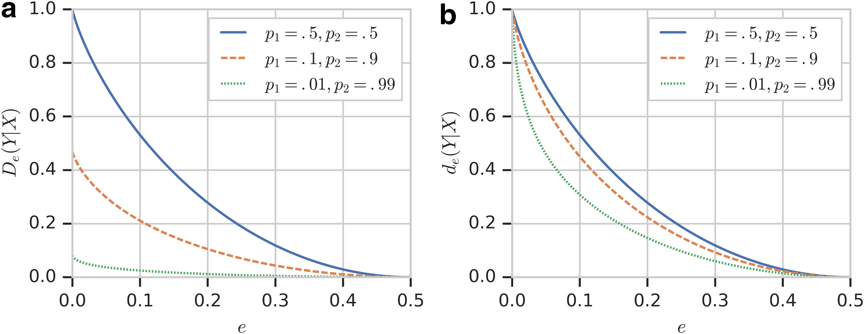
\end{document} given the probability distribution of p1 and p2. Figure 2a shows the relationship between the reliability function and error under three different probability distributions p(X). Note that the three curves shown in Figure 2a correspond to three slices through the surface in Figure 1.
Reliability function as a function of e. (a) The changes of reliability function \documentclass{aastex}\usepackage{amsbsy}\usepackage{amsfonts}\usepackage{amssymb}\usepackage{bm}\usepackage{mathrsfs}\usepackage{pifont}\usepackage{stmaryrd}\usepackage{textcomp}\usepackage{portland, xspace}\usepackage{amsmath, amsxtra}\usepackage{upgreek}\pagestyle{empty}\DeclareMathSizes{10}{9}{7}{6}\begin{document}
$${D_e} ( Y / X )$$
\end{document} with respect to e. The different line styles correspond to different probability distribution p(X): solid—p1 = 0.5, p2 = 0.5, dashed—p1 = 0.1, p2 = 0.9; and dotted—p1 = 0.01, p2 = 0.99. (b) The same information for normalized reliability function, \documentclass{aastex}\usepackage{amsbsy}\usepackage{amsfonts}\usepackage{amssymb}\usepackage{bm}\usepackage{mathrsfs}\usepackage{pifont}\usepackage{stmaryrd}\usepackage{textcomp}\usepackage{portland, xspace}\usepackage{amsmath, amsxtra}\usepackage{upgreek}\pagestyle{empty}\DeclareMathSizes{10}{9}{7}{6}\begin{document}
$${d_e} ( Y \vert X )$$
\end{document}.
Equation (8) shows that \documentclass{aastex}\usepackage{amsbsy}\usepackage{amsfonts}\usepackage{amssymb}\usepackage{bm}\usepackage{mathrsfs}\usepackage{pifont}\usepackage{stmaryrd}\usepackage{textcomp}\usepackage{portland, xspace}\usepackage{amsmath, amsxtra}\usepackage{upgreek}\pagestyle{empty}\DeclareMathSizes{10}{9}{7}{6}\begin{document}
$${D_e} ( Y \vert X )$$
\end{document} is bounded by 0 and \documentclass{aastex}\usepackage{amsbsy}\usepackage{amsfonts}\usepackage{amssymb}\usepackage{bm}\usepackage{mathrsfs}\usepackage{pifont}\usepackage{stmaryrd}\usepackage{textcomp}\usepackage{portland, xspace}\usepackage{amsmath, amsxtra}\usepackage{upgreek}\pagestyle{empty}\DeclareMathSizes{10}{9}{7}{6}\begin{document}
$$H ( X )$$
\end{document}, the entropy of the input variable. The reliability function should measure the effects of the missing values not the effect of the variable distribution; therefore, we normalize \documentclass{aastex}\usepackage{amsbsy}\usepackage{amsfonts}\usepackage{amssymb}\usepackage{bm}\usepackage{mathrsfs}\usepackage{pifont}\usepackage{stmaryrd}\usepackage{textcomp}\usepackage{portland, xspace}\usepackage{amsmath, amsxtra}\usepackage{upgreek}\pagestyle{empty}\DeclareMathSizes{10}{9}{7}{6}\begin{document}
$${D_e} ( Y \vert X )$$
\end{document} to ensure that the reliability function is between 0 and 1.
\documentclass{aastex}\usepackage{amsbsy}\usepackage{amsfonts}\usepackage{amssymb}\usepackage{bm}\usepackage{mathrsfs}\usepackage{pifont}\usepackage{stmaryrd}\usepackage{textcomp}\usepackage{portland, xspace}\usepackage{amsmath, amsxtra}\usepackage{upgreek}\pagestyle{empty}\DeclareMathSizes{10}{9}{7}{6}\begin{document}
\begin{align*}
{ d_e } ( Y \vert X ) = { \frac { { D_e } ( Y \vert X ) } { H ( X ) } } . \tag { 11 }
\end{align*}
\end{document}
Figure 2b shows how normalized reliability function \documentclass{aastex}\usepackage{amsbsy}\usepackage{amsfonts}\usepackage{amssymb}\usepackage{bm}\usepackage{mathrsfs}\usepackage{pifont}\usepackage{stmaryrd}\usepackage{textcomp}\usepackage{portland, xspace}\usepackage{amsmath, amsxtra}\usepackage{upgreek}\pagestyle{empty}\DeclareMathSizes{10}{9}{7}{6}\begin{document}
$${d_e} ( Y \vert X )$$
\end{document} depends on the error rate. Both \documentclass{aastex}\usepackage{amsbsy}\usepackage{amsfonts}\usepackage{amssymb}\usepackage{bm}\usepackage{mathrsfs}\usepackage{pifont}\usepackage{stmaryrd}\usepackage{textcomp}\usepackage{portland, xspace}\usepackage{amsmath, amsxtra}\usepackage{upgreek}\pagestyle{empty}\DeclareMathSizes{10}{9}{7}{6}\begin{document}
$${D_e} ( Y \vert X )$$
\end{document} and \documentclass{aastex}\usepackage{amsbsy}\usepackage{amsfonts}\usepackage{amssymb}\usepackage{bm}\usepackage{mathrsfs}\usepackage{pifont}\usepackage{stmaryrd}\usepackage{textcomp}\usepackage{portland, xspace}\usepackage{amsmath, amsxtra}\usepackage{upgreek}\pagestyle{empty}\DeclareMathSizes{10}{9}{7}{6}\begin{document}
$${d_e} ( Y \vert X )$$
\end{document} are actually symmetric with respect to error e. We focus, however, only on the realistic range of error rates, \documentclass{aastex}\usepackage{amsbsy}\usepackage{amsfonts}\usepackage{amssymb}\usepackage{bm}\usepackage{mathrsfs}\usepackage{pifont}\usepackage{stmaryrd}\usepackage{textcomp}\usepackage{portland, xspace}\usepackage{amsmath, amsxtra}\usepackage{upgreek}\pagestyle{empty}\DeclareMathSizes{10}{9}{7}{6}\begin{document}
$$0 \le e \le 0.5$$
\end{document}.
4.3. Simulations with pairwise dependence
Let us now examine the relationship between the reliability function and the amount of information as the frequency of missing values increases. To do this, we simulated data sets consisting of 200 variables that take on one of three values randomly across 1000 samples. All variables are independent except for the two special variables, X and Y, which are set to be identical for a given number of samples, thus forming a pairwise dependency. The fraction of samples for which X and Y are identical is referred to here as the strength of the dependency. In this simulation, we considered three cases: the strengths of dependency at 10%, 20%, and 50%.
To simulate missing data, as is often the case for real biological data, we removed 0%, 5%, 10%, 15%, and 20% of data points at random. Points for missing data were selected over all variables, including the dependent variables.
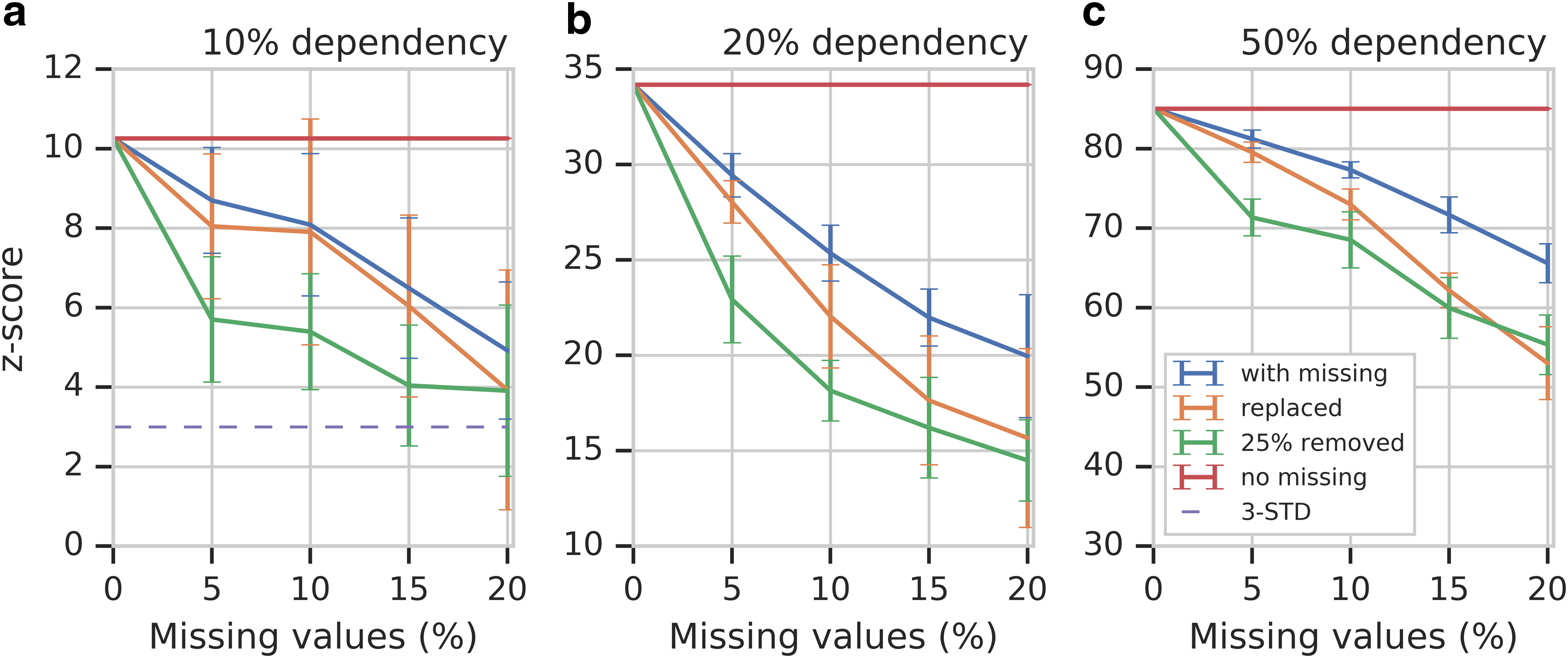
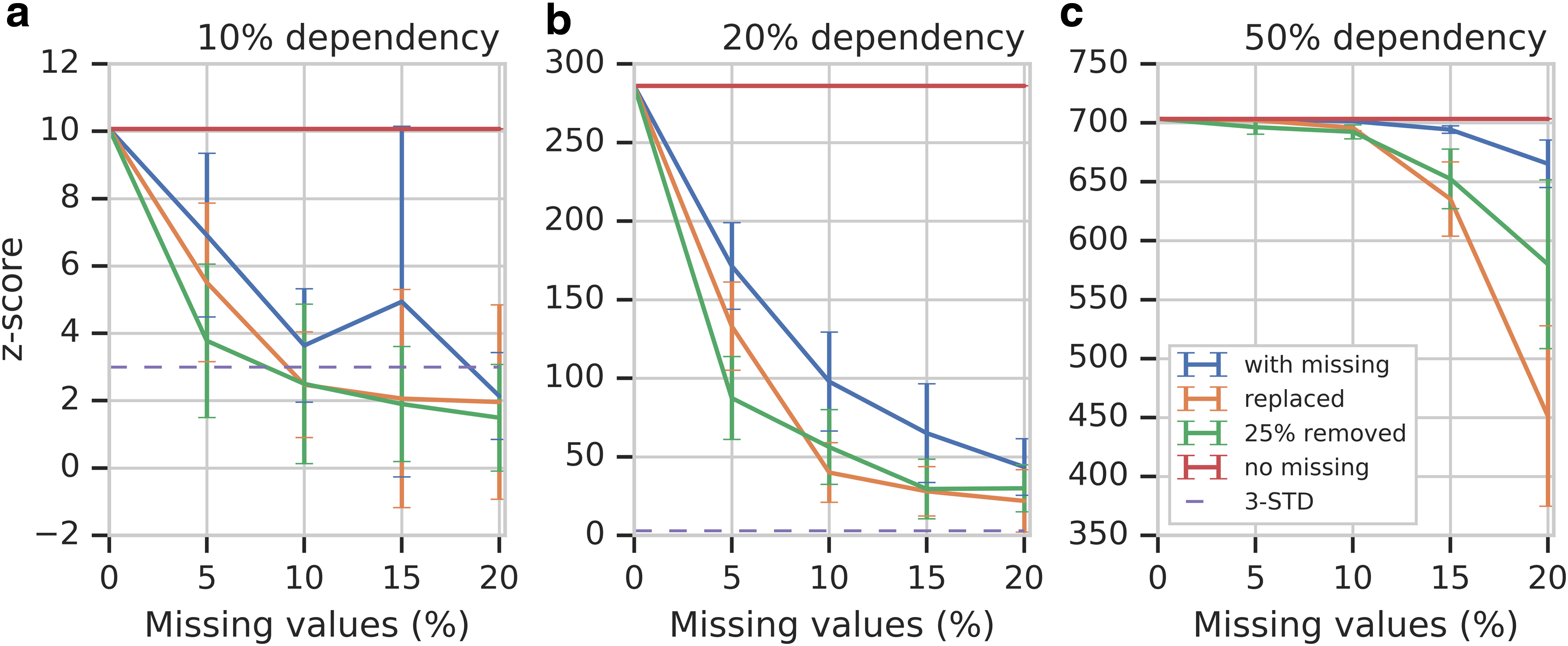
Given these simulated data, the task of interest is to detect the pairwise dependency between X and Y. We do this by simply computing mutual information for all possible pairs of variables and then identifying the pairs whose mutual information is significant. In this example, a pair is called significant if its z-score is >3. As expected, when there are no missing data, the dependency \documentclass{aastex}\usepackage{amsbsy}\usepackage{amsfonts}\usepackage{amssymb}\usepackage{bm}\usepackage{mathrsfs}\usepackage{pifont}\usepackage{stmaryrd}\usepackage{textcomp}\usepackage{portland, xspace}\usepackage{amsmath, amsxtra}\usepackage{upgreek}\pagestyle{empty}\DeclareMathSizes{10}{9}{7}{6}\begin{document}
$$\langle X , Y \rangle$$
\end{document} is highly significant (with z-score >80 when the dependency strength is 50%) and is the only significant pair. Figure 3 shows z-score of \documentclass{aastex}\usepackage{amsbsy}\usepackage{amsfonts}\usepackage{amssymb}\usepackage{bm}\usepackage{mathrsfs}\usepackage{pifont}\usepackage{stmaryrd}\usepackage{textcomp}\usepackage{portland, xspace}\usepackage{amsmath, amsxtra}\usepackage{upgreek}\pagestyle{empty}\DeclareMathSizes{10}{9}{7}{6}\begin{document}
$$\langle X , Y \rangle$$
\end{document} for various amounts of missing data and strengths of dependency.
z-Scores for various degrees of dependency in simulated data as a function of percentage missing data. The different curves represent the different options for dealing with missing data. The red line represents the case without any missing data, and the error bars represent the STD of the z-scores. Three other curves, blue, green, and orange, correspond to approaches (i), (ii), and (iii), respectively, to handling missing values. The dashed line indicates the three-STD level. (a–c) Correspond to the cases of 10%, 20%, and 50% dependencies. STD, standard deviation.
Section 3 discussed three different approaches for dealing with missing data that are common in biological data analysis. We evaluated all three of them as illustrated in Figure 3. Note that in approach (ii), we removed 25% of samples with the largest number of missing values, as shown in Appendix Figure A1 (Section 7.1).
As expected, Figure 3 shows that the increasing amount of missing data erodes the signal, reducing the significance of the dependency and making it harder to detect. Although the behavior of the approaches to handling the missing data is similar, approach (ii) generally performs the worst simply because removing many samples reduces the available information the most.
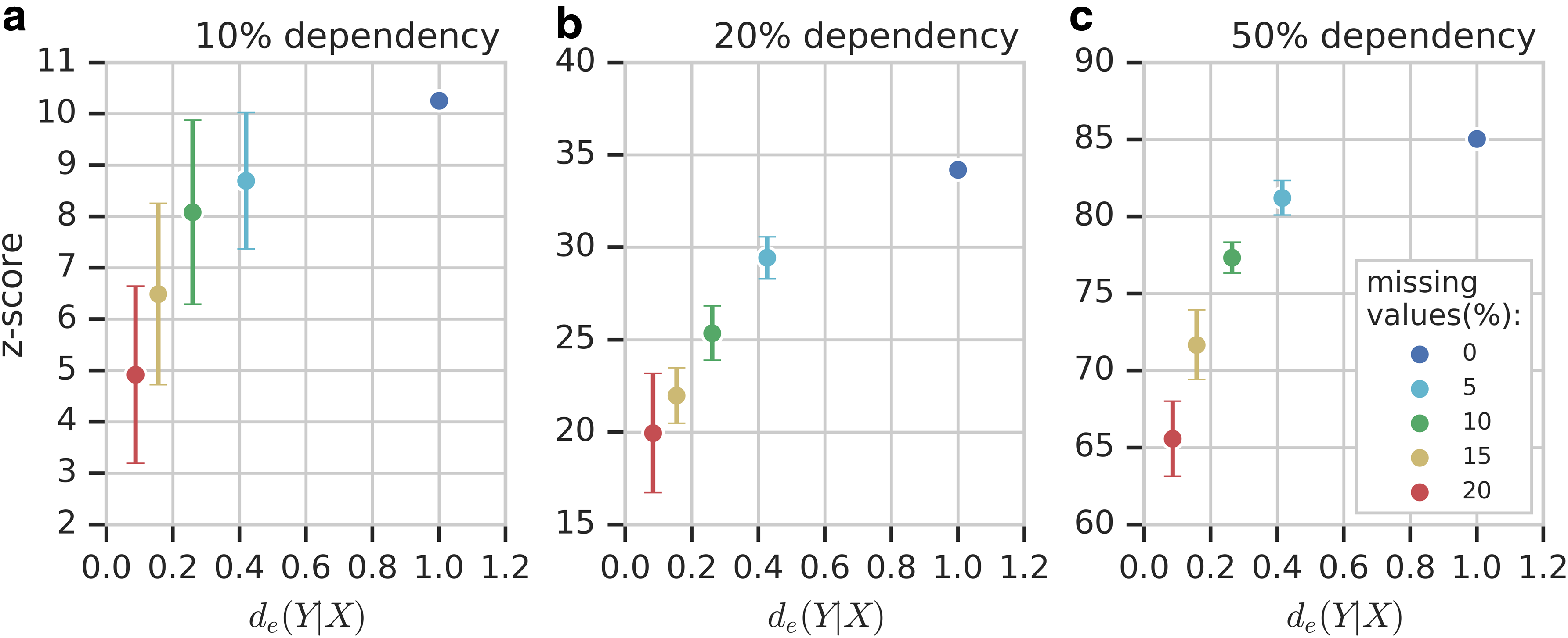
Let us now look at the (normalized) reliability functions of the dependent pair. Figure 4 shows the z-scores of \documentclass{aastex}\usepackage{amsbsy}\usepackage{amsfonts}\usepackage{amssymb}\usepackage{bm}\usepackage{mathrsfs}\usepackage{pifont}\usepackage{stmaryrd}\usepackage{textcomp}\usepackage{portland, xspace}\usepackage{amsmath, amsxtra}\usepackage{upgreek}\pagestyle{empty}\DeclareMathSizes{10}{9}{7}{6}\begin{document}
$$\langle X , Y \rangle$$
\end{document} versus the reliability function values with colors of the points corresponding to the number of missing values.
z-Score dependence on reliability function. Each panel shows the behavior of the z-scores when the values of the reliability function and frequency of the missing values change. The error bars represent the STD of the z-scores. The colors of circles correspond to the frequency of the missing values in a dependent tuple. (a–c) Correspond to the cases of 10%, 20%, and 50% dependencies.
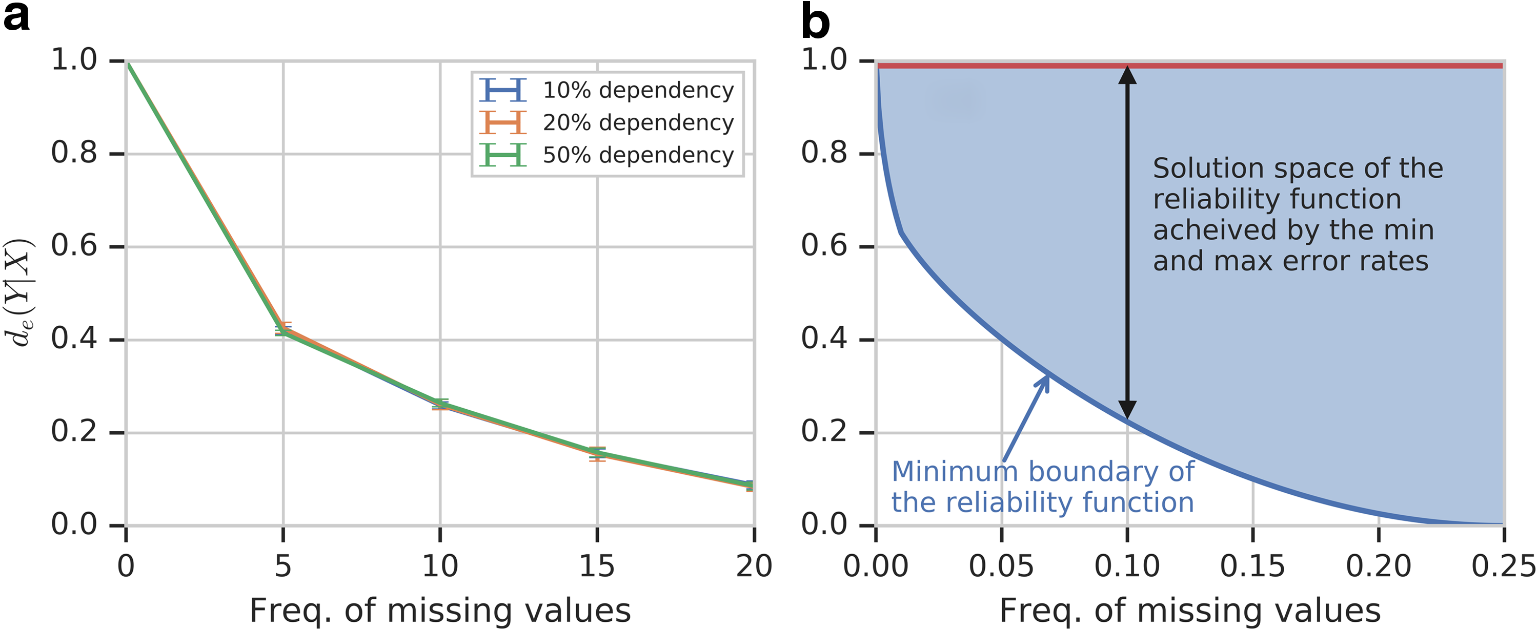
Note how the reliability function drops sharply as the amount of missing data goes from 0% to 5% and then slows down. Furthermore, the behavior of the reliability function when the missing data increase is largely independent of the strength of the dependency, as can be clearly seen in Figure 5, since the missing data are introduced into the data uniformly across all variables, including X and Y.
The normalized reliability function as a function of the frequency of missing values. (a) The function \documentclass{aastex}\usepackage{amsbsy}\usepackage{amsfonts}\usepackage{amssymb}\usepackage{bm}\usepackage{mathrsfs}\usepackage{pifont}\usepackage{stmaryrd}\usepackage{textcomp}\usepackage{portland, xspace}\usepackage{amsmath, amsxtra}\usepackage{upgreek}\pagestyle{empty}\DeclareMathSizes{10}{9}{7}{6}\begin{document}
$${d_e} ( Y \vert X )$$
\end{document} for all dependencies (mean of 10 independent simulations). They are identical. (b) The solution space.
Moreover, we can calculate the minimal possible value of the reliability function given the missing value level. The reliability function depends on the error rate: it has its minimal value when the error rate is maximal, which is equal to twice the rate of missing values. Calculating the reliability function with the maximal error rate results in the minimum boundary and the solution space of the reliability function shown in Figure 5.
5. Generalizing Reliability Function to Multiple Variables
In this section, we generalize the concept of a binary symmetric channel to the three-variable and then to the n-variable case. Similar to the pairwise case, we can derive the general n-variable reliability function expressed in terms of error rates, missing values, in the data.
5.1. The reliability function for three variables
Let us define the reliability function for the three-variable case, which measures the amount of information eroded by missing data when evaluating three-variable dependencies. We extend the transmission channel idea defined for two variables (Section 4) to three variables as follows. Let two of the variables represent two inputs, X1 and X2, and the other the output, Y. We refer to the output here as the “target” variable. Let us assume for the moment that the transmission of information through the channel is governed by the logical “OR” function, which for the error rate e results in the conditional probability given in Table 3.
Conditional Probability Table for the Three-Variable Case, Using “OR” Function Dependence
The “OR” function both models the information transmission in the presence of missing data and consistently parallels the pairwise case. The reliability function for three variables is then defined using the generalization of mutual information to three variables, which is called interaction information [Eq. (3)]. Using the definition of information transmission in the channel as given in Table 3, the reliability function can be expressed in terms of the joint probability of the inputs \documentclass{aastex}\usepackage{amsbsy}\usepackage{amsfonts}\usepackage{amssymb}\usepackage{bm}\usepackage{mathrsfs}\usepackage{pifont}\usepackage{stmaryrd}\usepackage{textcomp}\usepackage{portland, xspace}\usepackage{amsmath, amsxtra}\usepackage{upgreek}\pagestyle{empty}\DeclareMathSizes{10}{9}{7}{6}\begin{document}
$$p ( {X_1} , {X_2} )$$
\end{document} and the conditional probability \documentclass{aastex}\usepackage{amsbsy}\usepackage{amsfonts}\usepackage{amssymb}\usepackage{bm}\usepackage{mathrsfs}\usepackage{pifont}\usepackage{stmaryrd}\usepackage{textcomp}\usepackage{portland, xspace}\usepackage{amsmath, amsxtra}\usepackage{upgreek}\pagestyle{empty}\DeclareMathSizes{10}{9}{7}{6}\begin{document}
$$p ( Y \vert {X_1} , {X_2} )$$
\end{document} governing the noisy information transmission with error e:
\documentclass{aastex}\usepackage{amsbsy}\usepackage{amsfonts}\usepackage{amssymb}\usepackage{bm}\usepackage{mathrsfs}\usepackage{pifont}\usepackage{stmaryrd}\usepackage{textcomp}\usepackage{portland, xspace}\usepackage{amsmath, amsxtra}\usepackage{upgreek}\pagestyle{empty}\DeclareMathSizes{10}{9}{7}{6}\begin{document}
\begin{align*}
\begin{split} {D_e} ( Y \vert {X_1} , {X_2} ) = & - \mathop \sum \limits_{{x_1}} {p ( {x_1} ) \log [ p ( {x_1} ) ] } - \mathop \sum \limits_{{x_2}} {p ( {x_2} ) \log [ p ( {x_2} ) ] } \\ & + \mathop \sum \limits_{{x_1} , {x_2}} {p ( {x_1} , {x_2} ) \log [ p ( {x_1} , {x_2} ) ] } \\ & - \mathop \sum \limits_{{x_1} , {x_2} , y} {p ( y \vert {x_1} , {x_2} ) p ( {x_1} , {x_2} ) \log \left[ { \mathop \sum \limits_{{x_1} , {x_2}} {p ( y \vert {x_1} , {x_2} ) p ( {x_1} , {x_2} ) } } \right] } \\ & + \mathop \sum \limits_{{x_1} , {x_2} , y} {p ( y \vert {x_1} , {x_2} ) p ( {x_1} , {x_2} ) \log \left[ { \mathop \sum \limits_{{x_2}} {p ( y \vert {x_1} , {x_2} ) p ( {x_1} , {x_2} ) } } \right] } \\ & + \mathop \sum \limits_{{x_1} , {x_2} , y} {p ( y \vert {x_1} , {x_2} ) p ( {x_1} , {x_2} ) \log \left[ { \mathop \sum \limits_{{x_1}} {p ( y \vert {x_1} , {x_2} ) p ( {x_1} , {x_2} ) } } \right] } \\ & - \mathop \sum \limits_{{x_1} , {x_2} , y} {p ( y \vert {x_1} , {x_2} ) p ( {x_1} , {x_2} ) \log [ p ( y \vert {x_1} , {x_2} ) p ( {x_1} , {x_2} ) ] } . \end{split}
\tag{12}
\end{align*}
\end{document}
For the full derivation of the three-variable reliability function and its explicit expression in terms of e and elements \documentclass{aastex}\usepackage{amsbsy}\usepackage{amsfonts}\usepackage{amssymb}\usepackage{bm}\usepackage{mathrsfs}\usepackage{pifont}\usepackage{stmaryrd}\usepackage{textcomp}\usepackage{portland, xspace}\usepackage{amsmath, amsxtra}\usepackage{upgreek}\pagestyle{empty}\DeclareMathSizes{10}{9}{7}{6}\begin{document}
$$p ( {X_1} = 0 , \;{X_2} = 0 ) = {p_1}$$
\end{document}, \documentclass{aastex}\usepackage{amsbsy}\usepackage{amsfonts}\usepackage{amssymb}\usepackage{bm}\usepackage{mathrsfs}\usepackage{pifont}\usepackage{stmaryrd}\usepackage{textcomp}\usepackage{portland, xspace}\usepackage{amsmath, amsxtra}\usepackage{upgreek}\pagestyle{empty}\DeclareMathSizes{10}{9}{7}{6}\begin{document}
$$p ( {X_1} = 0 , \;{X_2} = 1 ) = {p_2}$$
\end{document}, \documentclass{aastex}\usepackage{amsbsy}\usepackage{amsfonts}\usepackage{amssymb}\usepackage{bm}\usepackage{mathrsfs}\usepackage{pifont}\usepackage{stmaryrd}\usepackage{textcomp}\usepackage{portland, xspace}\usepackage{amsmath, amsxtra}\usepackage{upgreek}\pagestyle{empty}\DeclareMathSizes{10}{9}{7}{6}\begin{document}
$$p ( {X_1} = 1 , \;{X_2} = 0 ) = {p_3}$$
\end{document}, and \documentclass{aastex}\usepackage{amsbsy}\usepackage{amsfonts}\usepackage{amssymb}\usepackage{bm}\usepackage{mathrsfs}\usepackage{pifont}\usepackage{stmaryrd}\usepackage{textcomp}\usepackage{portland, xspace}\usepackage{amsmath, amsxtra}\usepackage{upgreek}\pagestyle{empty}\DeclareMathSizes{10}{9}{7}{6}\begin{document}
$$p ( {X_1} = 1 , \;{X_2} = 1 ) = {p_4}$$
\end{document}, see Section 7.2.
Using set notation, Equation (12) can be represented more compactly as
where \documentclass{aastex}\usepackage{amsbsy}\usepackage{amsfonts}\usepackage{amssymb}\usepackage{bm}\usepackage{mathrsfs}\usepackage{pifont}\usepackage{stmaryrd}\usepackage{textcomp}\usepackage{portland, xspace}\usepackage{amsmath, amsxtra}\usepackage{upgreek}\pagestyle{empty}\DeclareMathSizes{10}{9}{7}{6}\begin{document}
$$\wp ( \{ {X_1} , {X_2} \} $$
\end{document} is a set of all subsets: \documentclass{aastex}\usepackage{amsbsy}\usepackage{amsfonts}\usepackage{amssymb}\usepackage{bm}\usepackage{mathrsfs}\usepackage{pifont}\usepackage{stmaryrd}\usepackage{textcomp}\usepackage{portland, xspace}\usepackage{amsmath, amsxtra}\usepackage{upgreek}\pagestyle{empty}\DeclareMathSizes{10}{9}{7}{6}\begin{document}
$$\{ \} , \{ {X_1} \} , \{ {X_2} \} $$
\end{document}, and \documentclass{aastex}\usepackage{amsbsy}\usepackage{amsfonts}\usepackage{amssymb}\usepackage{bm}\usepackage{mathrsfs}\usepackage{pifont}\usepackage{stmaryrd}\usepackage{textcomp}\usepackage{portland, xspace}\usepackage{amsmath, amsxtra}\usepackage{upgreek}\pagestyle{empty}\DeclareMathSizes{10}{9}{7}{6}\begin{document}
$$\{ {X_1} , \;{X_2} \} $$
\end{document}. Note that for simplicity, we write s to denote all possible combinations of values of variables in set S. Note also that the expression under the log of the second sum is marginalized over the variables of subset S.
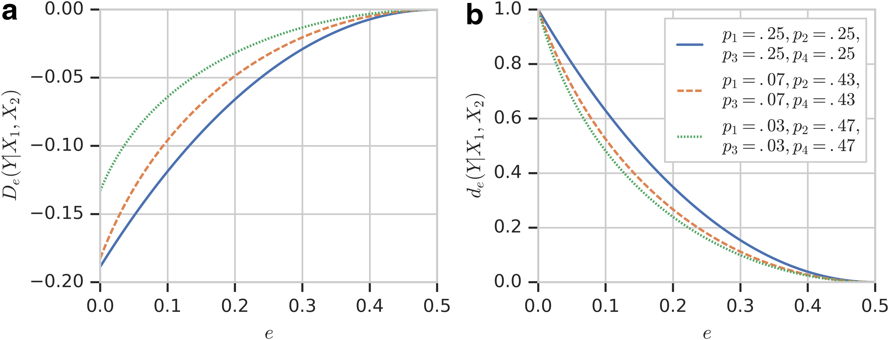
The normalization of the reliability function for three variables is given by Equation (15) in Section 5.3 as for n-variable formula. Figure 6 shows the relationship between the reliability function and error under three different probability distributions \documentclass{aastex}\usepackage{amsbsy}\usepackage{amsfonts}\usepackage{amssymb}\usepackage{bm}\usepackage{mathrsfs}\usepackage{pifont}\usepackage{stmaryrd}\usepackage{textcomp}\usepackage{portland, xspace}\usepackage{amsmath, amsxtra}\usepackage{upgreek}\pagestyle{empty}\DeclareMathSizes{10}{9}{7}{6}\begin{document}
$$p ( {X_1} , {X_2} )$$
\end{document}.
Reliability function as a function of e. (a) The changes of reliability function \documentclass{aastex}\usepackage{amsbsy}\usepackage{amsfonts}\usepackage{amssymb}\usepackage{bm}\usepackage{mathrsfs}\usepackage{pifont}\usepackage{stmaryrd}\usepackage{textcomp}\usepackage{portland, xspace}\usepackage{amsmath, amsxtra}\usepackage{upgreek}\pagestyle{empty}\DeclareMathSizes{10}{9}{7}{6}\begin{document}
$${D_e} ( Y \vert {X_1} , {X_2} )$$
\end{document} with respect to e. The different line styles correspond to different probability distribution \documentclass{aastex}\usepackage{amsbsy}\usepackage{amsfonts}\usepackage{amssymb}\usepackage{bm}\usepackage{mathrsfs}\usepackage{pifont}\usepackage{stmaryrd}\usepackage{textcomp}\usepackage{portland, xspace}\usepackage{amsmath, amsxtra}\usepackage{upgreek}\pagestyle{empty}\DeclareMathSizes{10}{9}{7}{6}\begin{document}
$$p ( {X_1} , {X_2} )$$
\end{document}: solid—p1 = 0.25, p2 = 0.25, p3 = 0.25, p4 = 0.25; dashed—p1 = 0.07, p2 = 0.43, p3 = 0.07, p4 = 0.43; and dotted—p1 = 0.03, p2 = 0.47, p3 = 0.03, p4 = 0.47. (b) The same information for normalized reliability function, \documentclass{aastex}\usepackage{amsbsy}\usepackage{amsfonts}\usepackage{amssymb}\usepackage{bm}\usepackage{mathrsfs}\usepackage{pifont}\usepackage{stmaryrd}\usepackage{textcomp}\usepackage{portland, xspace}\usepackage{amsmath, amsxtra}\usepackage{upgreek}\pagestyle{empty}\DeclareMathSizes{10}{9}{7}{6}\begin{document}
$${d_e} ( Y \vert {X_1} , {X_2} )$$
\end{document}.
Figure 6 shows the reliability function before (a) and after (b) normalization. Unlike the two-variable case, the values of \documentclass{aastex}\usepackage{amsbsy}\usepackage{amsfonts}\usepackage{amssymb}\usepackage{bm}\usepackage{mathrsfs}\usepackage{pifont}\usepackage{stmaryrd}\usepackage{textcomp}\usepackage{portland, xspace}\usepackage{amsmath, amsxtra}\usepackage{upgreek}\pagestyle{empty}\DeclareMathSizes{10}{9}{7}{6}\begin{document}
$${D_e} ( Y \vert {X_1} , {X_2} )$$
\end{document} become negative and convex upward, but also reach 0 at e = 0.5. In this case, the uniform probability distribution, p1 = p2 = p3 = p4, gives the minimum curve. Figure 6b shows the normalized reliability function. The normalized reliability function for three variables maintains the essential properties of the reliability function for two variables.
Rather than use the logical “OR” function to define the channel, another information transmission mode through the channel can be governed by the logical “AND” function. This leads to the conditional probability given in Table 4.
Conditional Probability Table for the Three-Variable Case with “AND” Function
As before, we calculate the reliability function and note that the symmetry of the table is reflected in the symmetry of the expression [Eq. (B4) in Section 7.2].
The normalization of the reliability function for three variables with “AND” function shows the same behavior as “OR” function because of their symmetry (Tables 3 and 4; Appendix Figure A2 in Section 7.1).
5.2. Simulated example with three-variable dependency
To illustrate the relationship between the reliability function and the amount of information when the frequency of missing values increases, we use the simulated example from Section 4.3 again, this time replacing the identity function with the logical XOR function to model the three-variable dependency. We kept all other parameters of the example same as in Section 4.3.
We first look at how much the increasing amount of missing data erodes the signal, reducing the significance of the dependency and making it harder to detect (Fig. 7). Note that this time we use interaction information (3) for all possible tuples and compare J(X,Y,Z) against the full set.
Reliability as a function of missing data. (a–c) The z-scores with respect to frequency of missing values for 10%, 20%, and 50% dependencies. The red line represents the case without any missing data, and the error bars represent the STD of the z-scores. Three other curves, blue, green, and orange, correspond to approaches (i), (ii), and (iii), respectively, to handling missing values. The dashed line indicates the three-STD level.
As in the pairwise case, the behavior of the three options for handling the missing data is similar, although the sample elimination approach defined in Appendix Figure A3 (in Section 7.1) performs worse simply because it is stricter, eliminating more information.
Following the pairwise example from Section 4, we examined the reliability function of the dependent pair. Appendix Figure A4 (in Section 7.1) shows the z-scores of \documentclass{aastex}\usepackage{amsbsy}\usepackage{amsfonts}\usepackage{amssymb}\usepackage{bm}\usepackage{mathrsfs}\usepackage{pifont}\usepackage{stmaryrd}\usepackage{textcomp}\usepackage{portland, xspace}\usepackage{amsmath, amsxtra}\usepackage{upgreek}\pagestyle{empty}\DeclareMathSizes{10}{9}{7}{6}\begin{document}
$$\langle {X_1} , {X_2} , Y \rangle$$
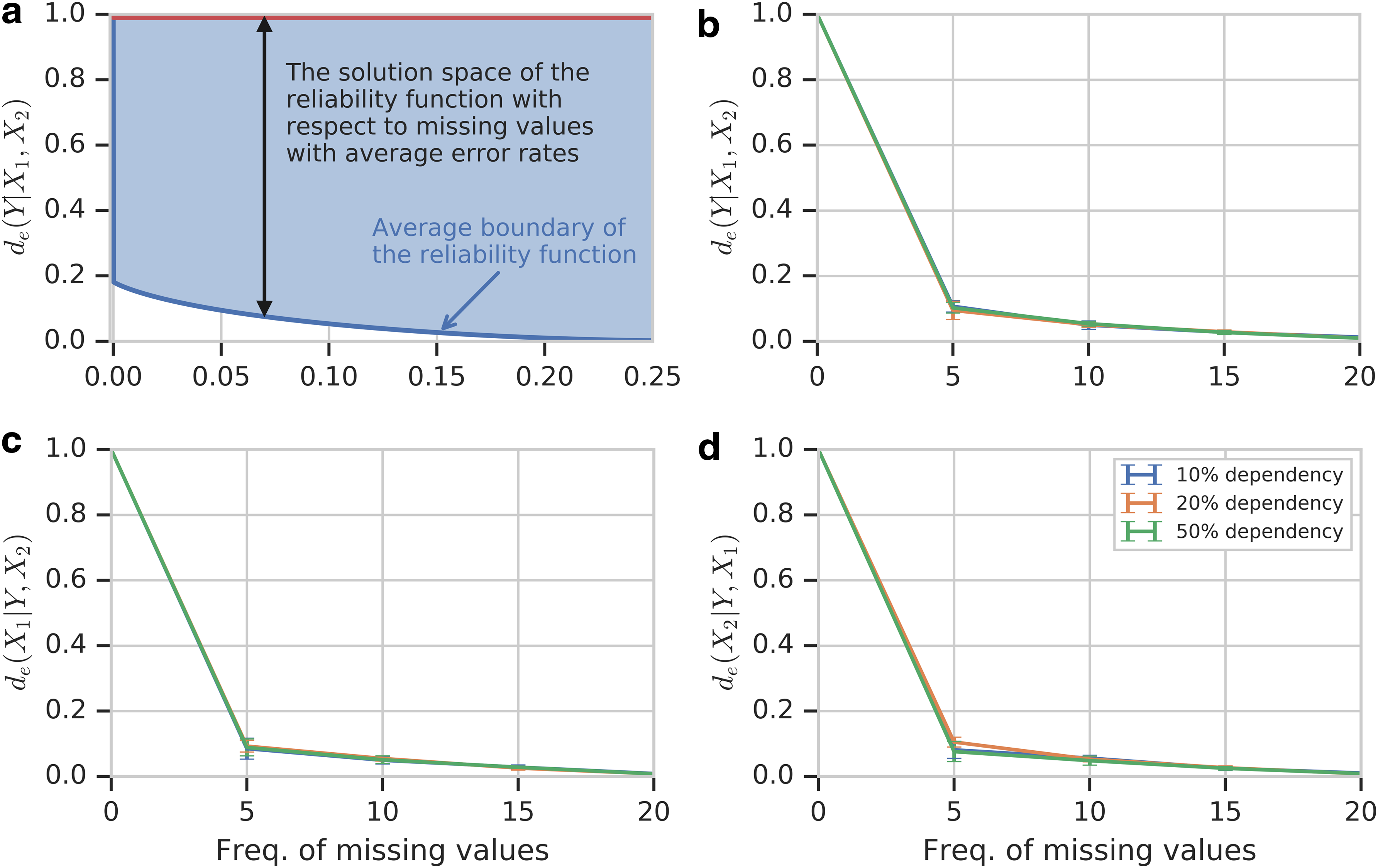
\end{document} versus the reliability function values, with colors corresponding to the number of missing values. Similar to the pairwise case, the reliability function drops sharply as the amount of missing data goes from 0% to 5% and then slows down. The normalized reliability function here is also independent of the strength of the dependency, as can be clearly seen in Figure 8.
Reliability function for three variable simulation (OR function.). (a) The solution space of the reliability function with respect to missing values given by average boundary of the reliability function. Unlike the two-variable case, the error rate and input probability in the three-variable reliability function are not directly defined by frequency of missing values. The average boundary of the reliability function is given instead of the minimum boundary. (b–d) The reliability function for three-variable versus frequency of missing values for different choices of target variable. The target variable is Y, X1, and X2, for (b–d).
Figure 8a also shows the minimal possible value of the reliability function, given the missing value level.
5.3. The reliability function for n variables
We can derive the reliability function for n variables, \documentclass{aastex}\usepackage{amsbsy}\usepackage{amsfonts}\usepackage{amssymb}\usepackage{bm}\usepackage{mathrsfs}\usepackage{pifont}\usepackage{stmaryrd}\usepackage{textcomp}\usepackage{portland, xspace}\usepackage{amsmath, amsxtra}\usepackage{upgreek}\pagestyle{empty}\DeclareMathSizes{10}{9}{7}{6}\begin{document}
$${V_n} = \{ {X_1} , {X_2} \ldots , {X_i} , \ldots , {X_{n}} \} $$
\end{document}, by using the interaction information and taking a target variable as Xi. Recall also that the interaction information is symmetric under permutation of the variables. Following the analysis of the three-variable case, we can directly formulate the general n-variable reliability function. As in the three-variable case, we extend the transmission channel idea from two variables to n variables. In this case, there are n−1 inputs and 1 output, also referred to as the “target” variable. The transmission of information through the channel is again governed by the logical OR function, as illustrated for three variables in Table 3. The logical OR function for N variables returns 1 if at least one of the input variables is equal to 1.
For simplicity, let us denote the set of all variables except Xi as Vn-1. Then the expression for \documentclass{aastex}\usepackage{amsbsy}\usepackage{amsfonts}\usepackage{amssymb}\usepackage{bm}\usepackage{mathrsfs}\usepackage{pifont}\usepackage{stmaryrd}\usepackage{textcomp}\usepackage{portland, xspace}\usepackage{amsmath, amsxtra}\usepackage{upgreek}\pagestyle{empty}\DeclareMathSizes{10}{9}{7}{6}\begin{document}
$${D_e} ( {X_i} \vert {V_{n - 1}} )$$
\end{document} in full, using set notation similar to (13) to accommodate the multiple variables, is given as follows:
where \documentclass{aastex}\usepackage{amsbsy}\usepackage{amsfonts}\usepackage{amssymb}\usepackage{bm}\usepackage{mathrsfs}\usepackage{pifont}\usepackage{stmaryrd}\usepackage{textcomp}\usepackage{portland, xspace}\usepackage{amsmath, amsxtra}\usepackage{upgreek}\pagestyle{empty}\DeclareMathSizes{10}{9}{7}{6}\begin{document}
$$\wp ( {V_{n - 1}} )$$
\end{document} is a set of all subsets of \documentclass{aastex}\usepackage{amsbsy}\usepackage{amsfonts}\usepackage{amssymb}\usepackage{bm}\usepackage{mathrsfs}\usepackage{pifont}\usepackage{stmaryrd}\usepackage{textcomp}\usepackage{portland, xspace}\usepackage{amsmath, amsxtra}\usepackage{upgreek}\pagestyle{empty}\DeclareMathSizes{10}{9}{7}{6}\begin{document}
$${V_{n - 1}}$$
\end{document}, including the empty set. Note that for simplicity we write νn to denote all possible n-variable combinations of values. Note also that the expression under the log of the second sum is marginalized over the variables of subset S.
5.3.1. Normalization
The meaning of the reliability function can be most clearly seen if we normalize it so that in the absence of missing information it goes to 1, and has a lower limit of 0. If we simply take the limit of zero error rate, \documentclass{aastex}\usepackage{amsbsy}\usepackage{amsfonts}\usepackage{amssymb}\usepackage{bm}\usepackage{mathrsfs}\usepackage{pifont}\usepackage{stmaryrd}\usepackage{textcomp}\usepackage{portland, xspace}\usepackage{amsmath, amsxtra}\usepackage{upgreek}\pagestyle{empty}\DeclareMathSizes{10}{9}{7}{6}\begin{document}
$${D_0} ( {X_i} \vert {V_{n - 1}} ) = { \lim \nolimits_{e \to 0}}{D_e} ( {X_i} \vert {V_{n - 1}} )$$
\end{document}, we can define the general normalized reliability function as the ratio
\documentclass{aastex}\usepackage{amsbsy}\usepackage{amsfonts}\usepackage{amssymb}\usepackage{bm}\usepackage{mathrsfs}\usepackage{pifont}\usepackage{stmaryrd}\usepackage{textcomp}\usepackage{portland, xspace}\usepackage{amsmath, amsxtra}\usepackage{upgreek}\pagestyle{empty}\DeclareMathSizes{10}{9}{7}{6}\begin{document}
\begin{align*}
{ d_e } \left( { { X_i } \vert { V_ { n - 1 } } } \right) = { \frac { { D_e } ( { X_i } \vert { V_ { n - 1 } } ) } { { D_0 } ( { X_i } \vert { V_ { n - 1 } } ) } } . \tag { 15 }
\end{align*}
\end{document}
In previous sections, we examined the properties of the reliability function for two and three variables in detail, and have shown how they can be used to handle missing values and evaluate measures calculated from incomplete data. Although we will not show results here, the general formulation for n variables can be applied in a similar manner.
6. Discussion and Conclusions
A reliability function based on information theory ideas is proposed here for use in evaluating results inferred from data sets with missing values. Since missing data are very common in biological and medical data sets, we need a rigorously consistent way to assess the specific effect of missing data on the results of inference of dependencies. In this article, we provide the way of using information theory methods to analyze this issue of missing data and define a reliability function based on the powerful metaphor of the channel capacity among variables. We view all variables in a data set as both sources and receivers of information during the analysis of a data set, defining pairwise and multiconnecting networks of variables as communication channels. The missing data are viewed as a noise or error source, and the analysis proceeds by quantitatively examining the communication between and among variables. The reliability function is identified with the channel capacity for the communication channels.
We began the article by treating the two-variable dependency case, showing a specific example of the pairwise dependency measure (mutual information) with incomplete data. In this case, we showed how the calculated mutual information, with missing data points, can distort the calculations and actually lead to negative mutual information. This, of course, is absurd and illustrates that significant problems can be caused by missing values. The values of mutual information calculated from incomplete data can also, of course, lead to falsely large or small values and result in false or missed signals of dependencies.
The concepts of a binary symmetric channel for two variables and the noise-channel capacity idea are generalized next for the case of n-variable dependencies, and a general definition of error rate for missing data is thus introduced. This reliability function for n-variable dependencies defines an error function, which in the case of a binary symmetric channel becomes the simple error rate. The reliability function can be simply normalized for any number of variables by comparison with the function in the limit of zero error rate.
Although our focus has been on the use of reliability functions in the application of our information-theoretic methods for the inference of dependencies, the pairwise case is equally applicable to other common methods such as regression and correlation methods. For the multivariable case, it is not entirely clear how to apply our approach to these methods.
Note also that we can think of using the reliability function in conjunction with a method for imputing the missing data. For example, the type of imputation (with or without prior knowledge) could be selected based on the value of the reliability function. This and other applications of the reliability function will be studied in our future work.
In summary, we have proposed a model of the reliability function that can assess the reliability of measures of multivariable dependencies based on the concepts of a binary symmetric channel. We expect that the methods described here can contribute to extracting as much information as possible from various types of biological data, allowing the use of data with missing values and enhance statistical properties of calculations of dependencies. This work thus contributes significantly to the general effort to find dependencies and interactions that exist in complex systems using data that may include missing values. We provide a general approach that can, in principle, deal with any data set, for any manner of complex system.
7. Appendix
7.1. Appendix A: Appendix figures
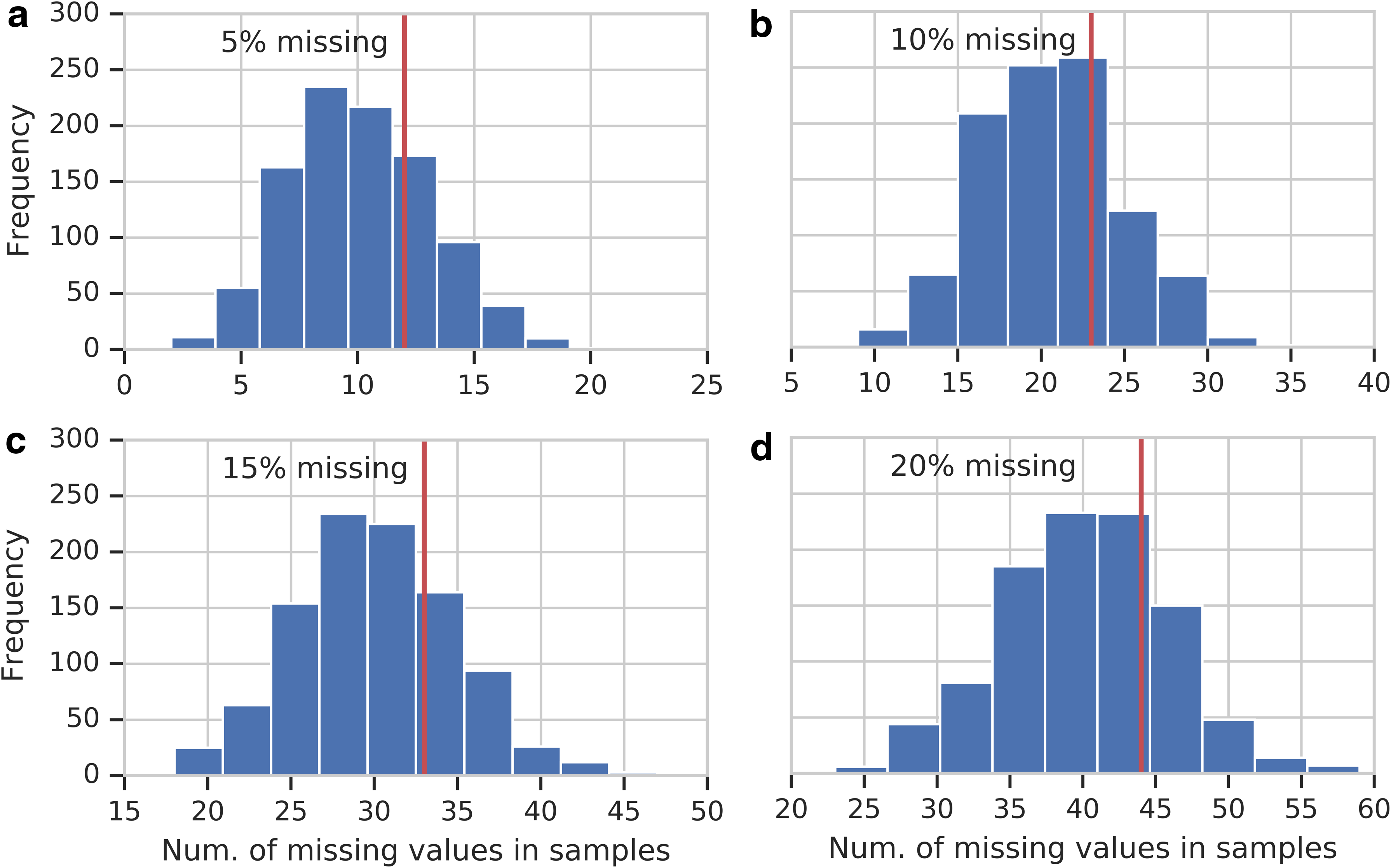
Appendix Figure A1 illustrates how the missing values are distributed in the simulated example of Section 4.3. It also shows how many samples are removed, when using approach (iii) for handling the missing data.
Distribution of missing values in simulations. All panels show histograms of missing values in samples included in data sets, which are used for mutual information calculation (Section 4.3). The frequency of missing values is 5%, 10%, 15%, and 20% for (a), (b), (c), and (d), respectively. The red line indicates the threshold of 75 percentile of missing values in a sample, which was the criterion for sample removal.
Appendix Figure A2 shows the behavior of the reliability function and its normalized version based on the AND function.
(a) The changes of reliability function De(Y|X1,X2) with respect to e calculated three-variable reliability function with AND function. The different line styles correspond to different probability distribution p(X1,X2): solid—p1 = 0.25, p2 = 0.25, p3 = 0.25, p4 = 0.25; dashed—p1 = 0.07, p2 = 0.43, p3 = 0.07, p4 = 0.43; and dotted—p1 = 0.03, p2 = 0.47, p3 = 0.03, p4 = 0.47. (b) The same information for normalized reliability function, de(Y|X1,X2).
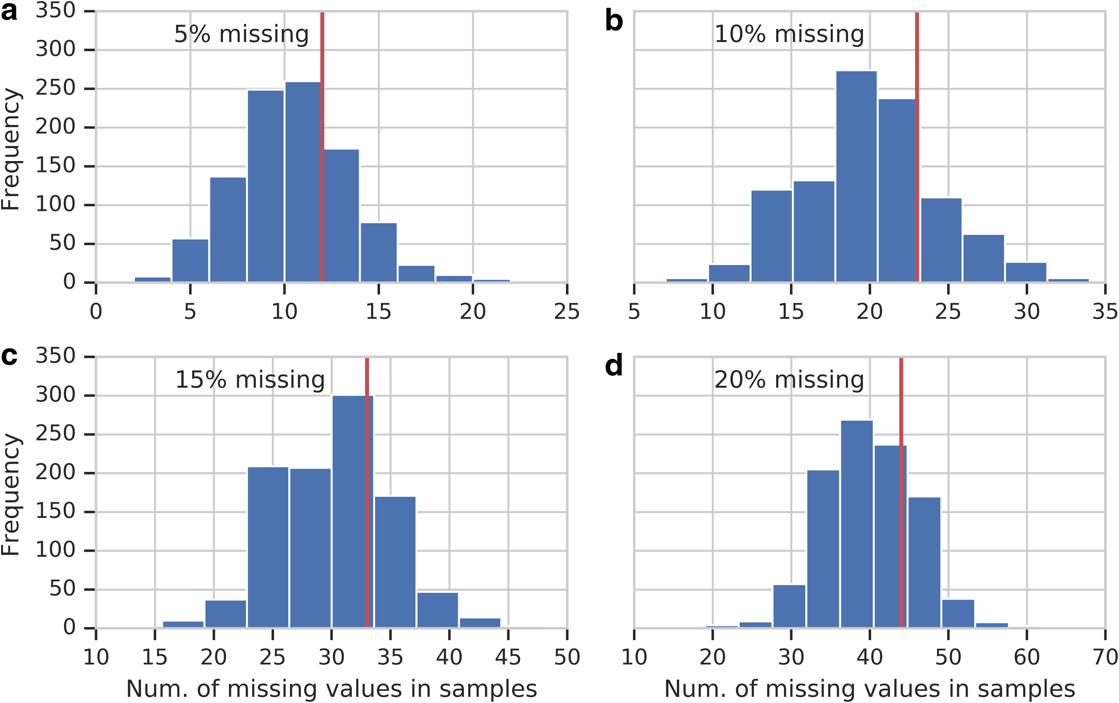
Appendix Figure A3 is similar to Appendix Figure A1. It illustrates how the missing values are distributed in the simulated example of Section 5.2. It also shows how many samples are removed, when using approach (iii) for handling the missing data.
Distribution of missing data in the three-variable simulation. Each panel shows histograms of missing values in samples included in data sets, which are used for Delta 3 calculation (Section 5.2). The frequency of missing values is 5%, 10%, 15%, and 20% for (a), (b), (c), and (d), respectively. The red line indicates the threshold of 75 percentile of missing values for sample removal.
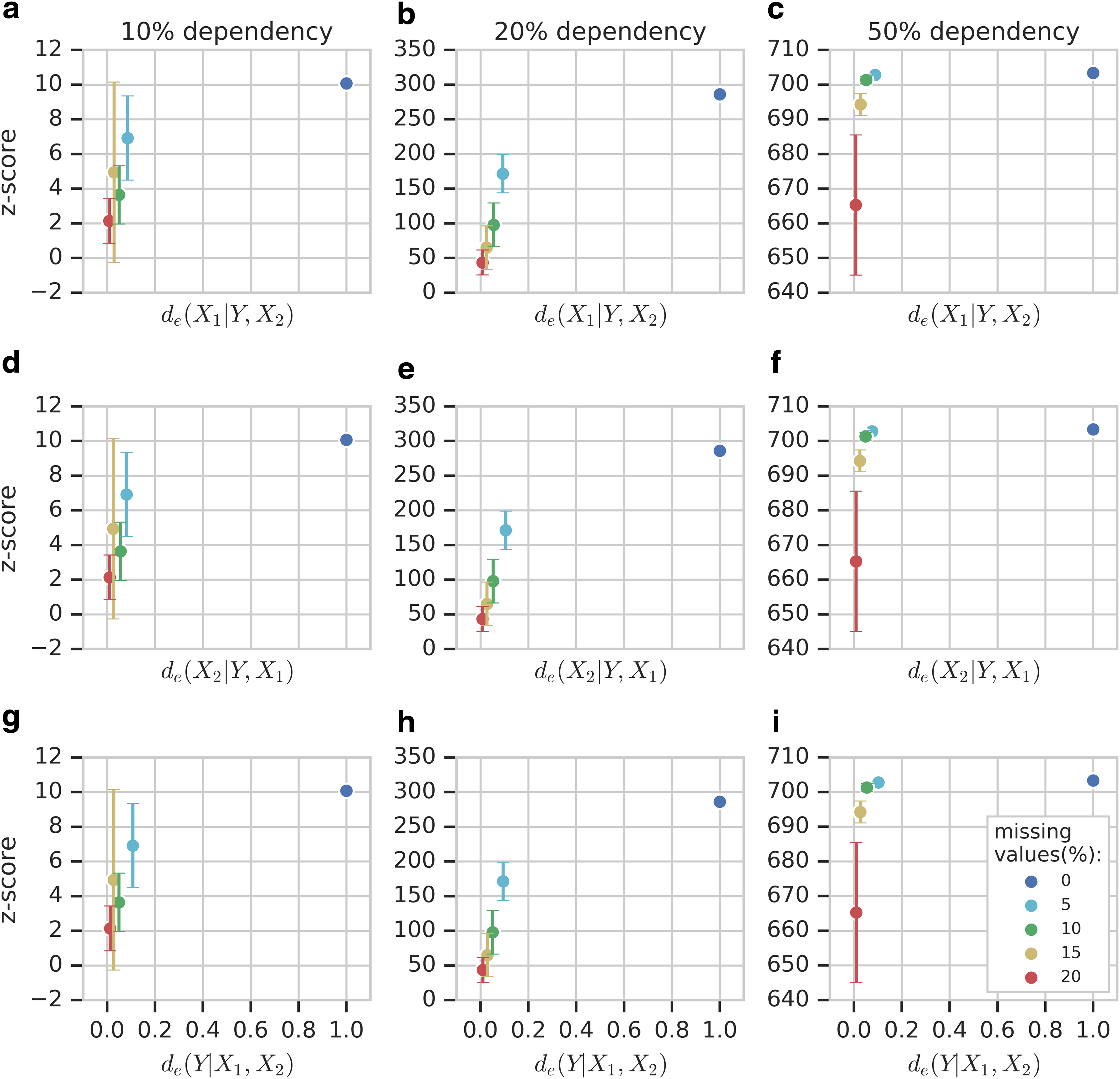
Appendix Figure A4 shows the z-scores of \documentclass{aastex}\usepackage{amsbsy}\usepackage{amsfonts}\usepackage{amssymb}\usepackage{bm}\usepackage{mathrsfs}\usepackage{pifont}\usepackage{stmaryrd}\usepackage{textcomp}\usepackage{portland, xspace}\usepackage{amsmath, amsxtra}\usepackage{upgreek}\pagestyle{empty}\DeclareMathSizes{10}{9}{7}{6}\begin{document}
$$\left\langle {{X_1} , {X_2} , Y} \right\rangle$$
\end{document} versus the reliability function values with colors of the points and error bars corresponding to the number of missing values from the simulated example of Section 5.2.
z-Score dependence on reliability function. (a–c)de(X1|Y,X2), (d–f)de(X2|Y,X1), and (g–i)de(Y|X1,X2). In contrast, three columns of panels correspond to three strength levels of the dependency, 10%, 20%, and 50%.
7.2. Appendix B: The reliability function for three variables
The reliability function for three variables is then defined using the generalization of mutual information to three variables, called interaction information [Eq. (3)]
\documentclass{aastex}\usepackage{amsbsy}\usepackage{amsfonts}\usepackage{amssymb}\usepackage{bm}\usepackage{mathrsfs}\usepackage{pifont}\usepackage{stmaryrd}\usepackage{textcomp}\usepackage{portland, xspace}\usepackage{amsmath, amsxtra}\usepackage{upgreek}\pagestyle{empty}\DeclareMathSizes{10}{9}{7}{6}\begin{document}
\begin{align*}
\begin{split} {D_e} ( Y \vert {X_1} , {X_2} ) & = I ( {X_1} , {X_2} , Y ) \\ & = - \mathop \sum \limits_{{x_1}} {p ( {x_1} ) \log [ p ( {x_1} ) ] } - \mathop \sum \limits_{{x_2}} {p ( {x_2} ) \log [ p ( {x_2} ) ] } \\ &\quad - \mathop \sum \limits_y {p ( y ) \log [ p ( y ) ] } \\ & \quad + \mathop \sum \limits_{{x_1} , {x_2}} {p ( {x_1} , {x_2} ) \log [ p ( {x_1} , {x_2} ) ] } \\ &\quad + \mathop \sum \limits_{{x_1} , y} {p ( {x_1} , y ) \log [ p ( {x_1} , y ) ] } + \mathop \sum \limits_{{x_2} , y} {p ( {x_2} , y ) \log [ p ( {x_2} , y ) ] } \\ & \quad - \mathop \sum \limits_{{x_1} , {x_2} , y} {p ( {x_1} , {x_2} , y ) \log [ p ( {x_1} , {x_2} , y ) ] } . \\ \end{split}
\tag{{ \rm B}1}
\end{align*}
\end{document}
Expressing the reliability function in terms of the marginal and joint probabilities of inputs p(X1,X2) and the conditional probability p(Y|X1,X2) governing the noisy information transmission with error e, we get
\documentclass{aastex}\usepackage{amsbsy}\usepackage{amsfonts}\usepackage{amssymb}\usepackage{bm}\usepackage{mathrsfs}\usepackage{pifont}\usepackage{stmaryrd}\usepackage{textcomp}\usepackage{portland, xspace}\usepackage{amsmath, amsxtra}\usepackage{upgreek}\pagestyle{empty}\DeclareMathSizes{10}{9}{7}{6}\begin{document}
\begin{align*}
\begin{split} {D_e} ( Y \vert {X_1} , {X_2} ) = & - \mathop \sum \limits_{{x_1}} {p ( {x_1} ) \log [ p ( {x_1} ) ] } - \mathop \sum \limits_{{x_2}} {p ( {x_2} ) \log [ p ( {x_2} ) ] } \\ & - \mathop \sum \limits_y { \left[ { \mathop \sum \limits_{{x_1} , {x_2}} {p ( y \vert {x_1} , {x_2} ) p ( {x_1} , {x_2} ) } } \right] \log \left[ { \mathop \sum \limits_{{x_1} , {x_2}} {p ( y \vert {x_1} , {x_2} ) p ( {x_1} , {x_2} ) } } \right] } \\ & + \mathop \sum \limits_{{x_1} , {x_2}} {p ( {x_1} , {x_2} ) \log [ p ( {x_1} , {x_2} ) ] } \\ & + \mathop \sum \limits_{{x_1} , y} { \left[ { \mathop \sum \limits_{{x_2}} {p ( y \vert {x_1} , {x_2} ) p ( {x_1} , {x_2} ) } } \right] \log \left[ { \mathop \sum \limits_{{x_2}} {p ( y \vert {x_1} , {x_2} ) p ( {x_1} , {x_2} ) } } \right] } \\ & + \mathop \sum \limits_{{x_2} , y} { \left[ { \mathop \sum \limits_{{x_1}} {p ( y \vert {x_1} , {x_2} ) p ( {x_1} , {x_2} ) } } \right] \log \left[ { \mathop \sum \limits_{{x_1}} {p ( y \vert {x_1} , {x_2} ) p ( {x_1} , {x_2} ) } } \right] } \\ & - \mathop \sum \limits_{{x_1} , {x_2} , y} {p ( y \vert {x_1} , {x_2} ) p ( {x_1} , {x_2} ) \log [ p ( y \vert {x_1} , {x_2} ) p ( {x_1} , {x_2} ) ] } . \\ \end{split}
\tag{{ \rm B}2}
\end{align*}
\end{document}
This can be further simplified resulting in Equation (12) in the main text of the article.
We are grateful to the members of the Galas group at PNRI for discussions. This work was partially supported by the Bill and Melinda Gates Foundation and the Pacific Northwest Research Institute.
Author Disclosure Statement
The authors declare that no competing financial interests exist.
References
1.
AdamiC., OfriaC., and CollierT.C.2000. Evolution of biological complexity. Proc. Natl. Acad. Sci. U.S.A. 97, 4463–4468.
2.
AshikhminA.E., BargA., and LitsynS.N.2000. A new upper bound on the reliability function of the Gaussian channel. IEEE Trans. Inf. Theory. 46, 1945–1961.
3.
CoverT.M., and ThomasJ.A.2012. Elements of Information Theory. John Wiley & Sons, New York, NY.
4.
DalyM.J., RiouxJ.D., SchaffnerS.F., et al.2001. High-resolution haplotype structure in the human genome. Nat. Genet. 29, 229–232.
5.
DoanR.N., BaeB.-I., CubelosB., et al.2016. Mutations in human accelerated regions disrupt cognition and social behavior. Cell. 167, 341–354.
6.
DoquireG., and VerleysenM.2011. Mutual information for feature selection with missing data, 269–274. Proceedings of the 19th European Symposium on Artificial Neural Networks, Computational Intelligence and Machine Learning, Bruges, Belgium.
7.
GalasD.J., NykterM., CarterG.W., et al.2010. Biological information as set-based complexity. IEEE Trans. Inf. Theory. 56, 667–677.
8.
GalasD.J., SakhanenkoN.A., SkupinA., et al.2014. Describing the complexity of systems: Multivariable “set complexity” and the information basis of systems biology. J. Comput. Biol. 21, 118–140.
9.
HudsonN.J., Porto-NetoL.R., KijasJ., et al.2014. Information compression exploits patterns of genome composition to discriminate populations and highlight regions of evolutionary interest. BMC Bioinformatics. 15, 66.
10.
HutterM., and ZaffalonM.2005. Distribution of mutual information from complete and incomplete data. Comput. Stat. Data Anal. 48, 633–657.
11.
KhinchinA.Y.1957. Mathematical Foundations of Information Theory. Courier Corporation., New York, NY.
12.
McGillW.J.1954. Multivariate information transmission. Psychometrika. 19, 97–116.
13.
PatilN., BernoA.J., HindsD.A., et al.2001. Blocks of limited haplotype diversity revealed by high-resolution scanning of human chromosome 21. Science. 294, 1719–1723.
14.
QianW., and ShuW.2015. Mutual information criterion for feature selection from incomplete data. Neurocomputing. 168, 210–220.
15.
Reyes-ValdesM.H., and WilliamsC.G.2005. An entropy-based measure of founder informativeness. Genet. Res. 85, 81–88.
16.
SakhanenkoN.A., and GalasD.J.2011. Interaction information in the discretization of quantitative phenotype data, 161–164. Proceeding of the 8th International Workshop on Computational Systems Biology, Zurich, Switzerland.
17.
SakhanenkoN.A., and GalasD.J.2015. Biological data analysis as an information theory problem: Multi-variable dependence measures and the shadows algorithm. J. Comput. Biol. 22, 1005–1024.
18.
SakhanenkoN.A., Kunert-GrafJ., and GalasD.J.2017. The information content of discrete functions and their application in genetic data analysis. J. Comput. Biol. 24, 1153–1178.
19.
ShannonC.E.1949. Communication in the presence of noise. Proc. IRE. 37, 10–21.
20.
ShannonC.E.2001. A mathematical theory of communication. SIGMOBILE Mob. Comput. Commun. Rev. 5, 3–55.
21.
SlonimN.2002. The information bottleneck: Theory and applications [Ph.D. dissertation]. Hebrew University of Jerusalem, Jerusalem, Israel.
22.
StephensM., and ScheetP.2005. Accounting for decay of linkage disequilibrium in haplotype inference and missing-data imputation. Am. J. Hum. Genet. 76, 449–462.
23.
SuS.C., KuoC.C., and ChenT.2005. Inference of missing SNPs and information quantity measurements for haplotype blocks. Bioinformatics. 21, 2001–2007.
24.
TishbyN., PereiraF.C., and BialekW.2000. The information bottleneck method. Comput. Res. Repository arXiv:physics/0004057.
25.
VerduS., and HanT.S.1994. A general formula for channel capacity. IEEE Trans. Inf. Theory. 40, 1147–1157.
26.
WengG., BhallaU.S., and IyengarR.1999. Complexity in biological signaling systems. Science. 284, 92–96.