Sage Journals: Discover world-class research

Abstract

An important feature of structural data, especially those from structural determination and protein-ligand docking programs, is that their distribution could be mostly uniform. Traditional clustering algorithms developed specifically for nonuniformly distributed data may not be adequate for their classification. Here we present a geometric partitional algorithm that could be applied to both uniformly and nonuniformly distributed data. The algorithm is a top-down approach that recursively selects the outliers as the seeds to form new clusters until all the structures within a cluster satisfy a classification criterion. The algorithm has been evaluated on a diverse set of real structural data and six sets of test data. The results show that it is superior to the previous algorithms for the clustering of structural data and is similar to or better than them for the classification of the test data. The algorithm should be especially useful for the identification of the best but minor clusters and for speeding up an iterative process widely used in NMR structure determination.

1. Introduction

Recently, we have witnessed a rapid growth of not only DNA sequencing data but also three-dimensional (3D) structural data such as those from biomolecular nuclear magnetic resonance (NMR) spectroscopy and protein-ligand docking as well as molecular dynamics (MD) simulation and protein structure prediction. These techniques output not a single but an ensemble of structures. A variety of traditional clustering algorithms both of hierarchical and partitional (Jain et al., 1999; Jain, 2010), being able to first assign the data points to groups (clusters) and then identify a representative for each cluster, have been applied to their analysis and visualization in order to discover or compare common structural features such as protein fold, binding site, and correct pose (May, 1999; Shao et al., 2007; Keller et al., 2010; Bottegoni et al., 2012; Adzhubei et al., 1995; Domingues et al., 2004; Sutcliffe, 1993; Downs and Barnard, 2002). However, it remains unclear which algorithm is most suitable for the clustering of 3D structural data because of the inherent difficulty associated with high dimensionality.* For example, a previous study concluded that there was no perfect “one size fits all” algorithm for the clustering of MD trajectories (Shao et al., 2007; and May, 1999) had questioned whether a hierarchical approach is appropriate for the clustering of structural data by forcing them into a dendrogram.

An important feature of structural data, especially those from NMR structural determination and protein-ligand docking, is that their distribution could be mostly uniform, and thus may not be properly described by a Gaussian mixture model. Traditional clustering algorithms developed specifically for nonuniformly distributed data may not be adequate for their classification. In this article, we present a novel geometric partitional algorithm that could be applied to both uniformly and nonuniformly distributed data. The algorithm is a top-down approach that recursively partitions all the data points of a previously generated cluster into c new clusters where c is a user-specified number. It stops and then outputs a final set of clusters that satisfy the classification criterion that no metric distances between any pair of data points in any cluster are larger than a certain value. Compared with the previous clustering algorithms, the salient features of our geometric partitional algorithm are (a) it uses the global information in the beginning, (b) it can handle both uniformly and nonuniformly distributed data, and (c) it is deterministic.

We have applied the algorithm to the classification of a diverse set of data: the intermediate structures from an NMR structure determination project, poses from protein-ligand docking, and MD trajectories from an ab-initio protein folding simulation (data not shown), as well as six sets of test data that have been used widely for the evaluation of clustering algorithms. We have also compared the algorithm with the following five different clustering algorithms: common nearest-neighbor, bipartition, complete-link, average-link, and k-medoids, on both real structural data and test data. The results show that our algorithm classifies the structural data with a higher accuracy than a k-medoids does. For the structural data sets, though the final set of clusters from our algorithm may be similar to those from a hierarchical algorithm such as complete-link or average-link, and to those from a nearest-neighbor or bipartition algorithm, the structures assigned to the same cluster by our algorithm are more uniform in terms of their structural and physical properties.

More importantly, our algorithm outperforms the previous ones in singling out the minor clusters with “good” properties (the best or correct clusters) that are often to be overlooked or even discarded by other criteria used for the selection of representative structures. Furthermore, the comparisons of our algorithm with the above five algorithms on the test data sets confirm its generality: the algorithm performs as well as or better than the previous ones in their classification. The rest of the article is organized as follows. In section 2 we first present the algorithm and then describe the real structural data sets. In section 3 we present the results of applying both our algorithm and five previous algorithms to the structural data sets for the identification of the clusters with good scores, and discuss the significance of the geometric algorithm for speeding up the iterative NMR structure determination process and for the selection of accurate docking poses. In section 4 we compare our clustering algorithm with the previous ones from both the theoretical and practical perspectives. Finally, we conclude the article with a section on the challenges of structural data classification.

2. The Algorithm and Data Set

In this section, we first present our novel geometric partitional algorithm for the clustering of structural data. Then we describe the data sets used for assessing the performance of the new and five previous clustering algorithms.

2.1. The geometric partitional algorithm

The similarity metric Our algorithm employs a recursive top-down procedure that clusters a set of structures (data points) S using the pairwise root-mean square distance (RMSD) d_ij between two structures i, j as a similarity metric, though other metrics could also be used. All the pairwise d_ijs are precomputed and saved in set D.

The algorithm The algorithm itself proceeds as follows. Let \documentclass{aastex}\usepackage{amsbsy}\usepackage{amsfonts}\usepackage{amssymb}\usepackage{bm}\usepackage{mathrsfs}\usepackage{pifont}\usepackage{stmaryrd}\usepackage{textcomp}\usepackage{portland, xspace}\usepackage{amsmath, amsxtra}\pagestyle{empty}\DeclareMathSizes{10}{9}{7}{6}\begin{document} $${\mathbb C}_s$$ \end{document} denote the set of clusters at recursive step s that have been generated at an earlier step s −1. At the initial step \documentclass{aastex}\usepackage{amsbsy}\usepackage{amsfonts}\usepackage{amssymb}\usepackage{bm}\usepackage{mathrsfs}\usepackage{pifont}\usepackage{stmaryrd}\usepackage{textcomp}\usepackage{portland, xspace}\usepackage{amsmath, amsxtra}\pagestyle{empty}\DeclareMathSizes{10}{9}{7}{6}\begin{document} $$s = 1 , {\mathbb C}_1$$ \end{document} has only a single cluster S to which all the data belong. At step s, for each cluster \documentclass{aastex}\usepackage{amsbsy}\usepackage{amsfonts}\usepackage{amssymb}\usepackage{bm}\usepackage{mathrsfs}\usepackage{pifont}\usepackage{stmaryrd}\usepackage{textcomp}\usepackage{portland, xspace}\usepackage{amsmath, amsxtra}\pagestyle{empty}\DeclareMathSizes{10}{9}{7}{6}\begin{document} $${\bf C} \in {\mathbb C}_s$$ \end{document} , the algorithm first computes m points, \documentclass{aastex}\usepackage{amsbsy}\usepackage{amsfonts}\usepackage{amssymb}\usepackage{bm}\usepackage{mathrsfs}\usepackage{pifont}\usepackage{stmaryrd}\usepackage{textcomp}\usepackage{portland, xspace}\usepackage{amsmath, amsxtra}\pagestyle{empty}\DeclareMathSizes{10}{9}{7}{6}\begin{document} $${\bf c}_ \mu \in {\bf C} , \mu = 1 , \ldots , m$$ \end{document} , as the seeds for m new clusters, \documentclass{aastex}\usepackage{amsbsy}\usepackage{amsfonts}\usepackage{amssymb}\usepackage{bm}\usepackage{mathrsfs}\usepackage{pifont}\usepackage{stmaryrd}\usepackage{textcomp}\usepackage{portland, xspace}\usepackage{amsmath, amsxtra}\pagestyle{empty}\DeclareMathSizes{10}{9}{7}{6}\begin{document} $${\bf C}_{\mu} \in {\mathbb C}_{s + 1} , \mu = 1 , \ldots , m$$ \end{document} , and then uniquely assigns all the remaining points in C to \documentclass{aastex}\usepackage{amsbsy}\usepackage{amsfonts}\usepackage{amssymb}\usepackage{bm}\usepackage{mathrsfs}\usepackage{pifont}\usepackage{stmaryrd}\usepackage{textcomp}\usepackage{portland, xspace}\usepackage{amsmath, amsxtra}\pagestyle{empty}\DeclareMathSizes{10}{9}{7}{6}\begin{document} $${\bf C}_{\mu} \in {\mathbb C}_{s + 1} , \mu = 1 , \ldots , m$$ \end{document} where 3 ≤ m ≤ N_c while N_c is a user-specified number. The above m seed points are defined and computed as follows. The first two points, c₁ and c₂, whose RMSD is the largest among all the pairwise d_ijs in cluster \documentclass{aastex}\usepackage{amsbsy}\usepackage{amsfonts}\usepackage{amssymb}\usepackage{bm}\usepackage{mathrsfs}\usepackage{pifont}\usepackage{stmaryrd}\usepackage{textcomp}\usepackage{portland, xspace}\usepackage{amsmath, amsxtra}\pagestyle{empty}\DeclareMathSizes{10}{9}{7}{6}\begin{document} $${\bf C} \in {\mathbb C}_s$$ \end{document} , seed the first two clusters, \documentclass{aastex}\usepackage{amsbsy}\usepackage{amsfonts}\usepackage{amssymb}\usepackage{bm}\usepackage{mathrsfs}\usepackage{pifont}\usepackage{stmaryrd}\usepackage{textcomp}\usepackage{portland, xspace}\usepackage{amsmath, amsxtra}\pagestyle{empty}\DeclareMathSizes{10}{9}{7}{6}\begin{document} $${\bf C}_1 \in {\mathbb C}_{s + 1}$$ \end{document} and \documentclass{aastex}\usepackage{amsbsy}\usepackage{amsfonts}\usepackage{amssymb}\usepackage{bm}\usepackage{mathrsfs}\usepackage{pifont}\usepackage{stmaryrd}\usepackage{textcomp}\usepackage{portland, xspace}\usepackage{amsmath, amsxtra}\pagestyle{empty}\DeclareMathSizes{10}{9}{7}{6}\begin{document} $${\bf C}_2 \in {\mathbb C}_{s + 1}$$ \end{document} . A point c₃ in C−{c₁, c₂} that may seed a new cluster, the third cluster \documentclass{aastex}\usepackage{amsbsy}\usepackage{amsfonts}\usepackage{amssymb}\usepackage{bm}\usepackage{mathrsfs}\usepackage{pifont}\usepackage{stmaryrd}\usepackage{textcomp}\usepackage{portland, xspace}\usepackage{amsmath, amsxtra}\pagestyle{empty}\DeclareMathSizes{10}{9}{7}{6}\begin{document} $${\bf C}_3 \in {\mathbb C}_{s + 1}$$ \end{document} , is the point that together with the above two points c₁, c₂ form a triangle with the largest area among all the triangles in C−{c₁, c₂}. Similarly, a point c₄ in C−{c₁, c₂, c₃} that may seed a new cluster, the fourth cluster \documentclass{aastex}\usepackage{amsbsy}\usepackage{amsfonts}\usepackage{amssymb}\usepackage{bm}\usepackage{mathrsfs}\usepackage{pifont}\usepackage{stmaryrd}\usepackage{textcomp}\usepackage{portland, xspace}\usepackage{amsmath, amsxtra}\pagestyle{empty}\DeclareMathSizes{10}{9}{7}{6}\begin{document} $${\bf C}_4 \in {\mathbb C}_{s + 1}$$ \end{document} , is the point that together with the above c₁, c₂, c₃ form a tetrahedron with the largest volume among the tetrahedrons formed by all the quadruples consisting of c₁, c₂, c₃ and a point in C−{c₁, c₂, c₃}. Finally, a point c_m in \documentclass{aastex}\usepackage{amsbsy}\usepackage{amsfonts}\usepackage{amssymb}\usepackage{bm}\usepackage{mathrsfs}\usepackage{pifont}\usepackage{stmaryrd}\usepackage{textcomp}\usepackage{portland, xspace}\usepackage{amsmath, amsxtra}\pagestyle{empty}\DeclareMathSizes{10}{9}{7}{6}\begin{document} $${\bf C} - \{{\bf c}_1 , {\bf c}_2 , \ldots , {\bf c}_{m - 1} \} $$ \end{document} may seed the last cluster \documentclass{aastex}\usepackage{amsbsy}\usepackage{amsfonts}\usepackage{amssymb}\usepackage{bm}\usepackage{mathrsfs}\usepackage{pifont}\usepackage{stmaryrd}\usepackage{textcomp}\usepackage{portland, xspace}\usepackage{amsmath, amsxtra}\pagestyle{empty}\DeclareMathSizes{10}{9}{7}{6}\begin{document} $${\bf C}_m \in {\mathbb C}_{s + 1}$$ \end{document} that together with \documentclass{aastex}\usepackage{amsbsy}\usepackage{amsfonts}\usepackage{amssymb}\usepackage{bm}\usepackage{mathrsfs}\usepackage{pifont}\usepackage{stmaryrd}\usepackage{textcomp}\usepackage{portland, xspace}\usepackage{amsmath, amsxtra}\pagestyle{empty}\DeclareMathSizes{10}{9}{7}{6}\begin{document} $$\{{\bf c}_1 , \ldots , {\bf c}_{m - 1} \} $$ \end{document} form a polyhedron that has the largest Cayley-Menger determinant (Blumenthal, 1970) among the polyhedra formed by all the m-tuples consisting of \documentclass{aastex}\usepackage{amsbsy}\usepackage{amsfonts}\usepackage{amssymb}\usepackage{bm}\usepackage{mathrsfs}\usepackage{pifont}\usepackage{stmaryrd}\usepackage{textcomp}\usepackage{portland, xspace}\usepackage{amsmath, amsxtra}\pagestyle{empty}\DeclareMathSizes{10}{9}{7}{6}\begin{document} $$\{{\bf c}_1 , \ldots , {\bf c}_{m - 1} \} $$ \end{document} and a point from \documentclass{aastex}\usepackage{amsbsy}\usepackage{amsfonts}\usepackage{amssymb}\usepackage{bm}\usepackage{mathrsfs}\usepackage{pifont}\usepackage{stmaryrd}\usepackage{textcomp}\usepackage{portland, xspace}\usepackage{amsmath, amsxtra}\pagestyle{empty}\DeclareMathSizes{10}{9}{7}{6}\begin{document} $${\bf C} - \{{\bf c}_1 , {\bf c}_2 , \ldots , {\bf c}_{m - 1} \} $$ \end{document} . For each point \documentclass{aastex}\usepackage{amsbsy}\usepackage{amsfonts}\usepackage{amssymb}\usepackage{bm}\usepackage{mathrsfs}\usepackage{pifont}\usepackage{stmaryrd}\usepackage{textcomp}\usepackage{portland, xspace}\usepackage{amsmath, amsxtra}\pagestyle{empty}\DeclareMathSizes{10}{9}{7}{6}\begin{document} $$p \in {\bf C} - \{{\bf c}_1 , {\bf c}_2 , \ldots , {\bf c}_{m} \} $$ \end{document} the algorithm assigns it to the kth cluster \documentclass{aastex}\usepackage{amsbsy}\usepackage{amsfonts}\usepackage{amssymb}\usepackage{bm}\usepackage{mathrsfs}\usepackage{pifont}\usepackage{stmaryrd}\usepackage{textcomp}\usepackage{portland, xspace}\usepackage{amsmath, amsxtra}\pagestyle{empty}\DeclareMathSizes{10}{9}{7}{6}\begin{document} $${\bf C}_{k} \in {\mathbb C}_{s + 1}$$ \end{document} where k is determined by \documentclass{aastex}\usepackage{amsbsy}\usepackage{amsfonts}\usepackage{amssymb}\usepackage{bm}\usepackage{mathrsfs}\usepackage{pifont}\usepackage{stmaryrd}\usepackage{textcomp}\usepackage{portland, xspace}\usepackage{amsmath, amsxtra}\pagestyle{empty}\DeclareMathSizes{10}{9}{7}{6}\begin{document} \begin{align*}\mathop{\arg \min\limits_k} d_{p{\bf C}_{k}} , \quad k = 1 , \ldots , m \tag{1}\end{align*} \end{document}

where \documentclass{aastex}\usepackage{amsbsy}\usepackage{amsfonts}\usepackage{amssymb}\usepackage{bm}\usepackage{mathrsfs}\usepackage{pifont}\usepackage{stmaryrd}\usepackage{textcomp}\usepackage{portland, xspace}\usepackage{amsmath, amsxtra}\pagestyle{empty}\DeclareMathSizes{10}{9}{7}{6}\begin{document} $$d_{p{\bf C}_{k}}$$ \end{document} is the RMSD between p and the seed c_k.

In the following we present the key steps of the algorithm at recursive step s with an input one of clusters \documentclass{aastex}\usepackage{amsbsy}\usepackage{amsfonts}\usepackage{amssymb}\usepackage{bm}\usepackage{mathrsfs}\usepackage{pifont}\usepackage{stmaryrd}\usepackage{textcomp}\usepackage{portland, xspace}\usepackage{amsmath, amsxtra}\pagestyle{empty}\DeclareMathSizes{10}{9}{7}{6}\begin{document} $${\bf C} \in {\mathbb C}_s$$ \end{document} generated at step s−1 and with N_c=4.

1. Search for the first two seed points, c₁ and c₂, whose metric d₁₂ \documentclass{aastex}\usepackage{amsbsy}\usepackage{amsfonts}\usepackage{amssymb}\usepackage{bm}\usepackage{mathrsfs}\usepackage{pifont}\usepackage{stmaryrd}\usepackage{textcomp}\usepackage{portland, xspace}\usepackage{amsmath, amsxtra}\pagestyle{empty}\DeclareMathSizes{10}{9}{7}{6}\begin{document} $$\in {\bf D}$$ \end{document} is the largest among all the pairs of structures in C

2. If d₁₂ ≤ d_max

Stop {no new clusters}

3. Initialize two new clusters C₁ and C₂ with c₁ and c₂ as their respective seeds

4. Search for the third seed point c₃ in C−{c₁, c₂} that together with c₁, c₂ forms a triangle with the largest area among all the possible triangles

5. If any of d₁₃ and d₂₃ is smaller than d_max

(a) For each point p in C−{c₁, c₂}

Assign it to C₁ if d_p_c1 ≤ d_p_c2, otherwise to C₂

(b) For both clusters C₁ and C₂

Go to Step 1

6. Seed a third cluster C₃ with c₃

7. Search for the fourth seed point c₄ in C−{c₁, c₂, c₃} that together with c₁, c₂, c₃ forms a tetrahedron with the largest volume among all the possible tetrahedrons

8. If any of d₁₄, d₂₄, d₃₄ is smaller than d_max

(a) Assign each point p in C−{c₁, c₂, c₃} to either C₁, C₂, C₃ according to equation (1)

(b) For each cluster C_j, j=1, 2, 3.

Go to Step 1

9. Else

(a) Seed a cluster C₄ with c₄

(b) Assign each point p in C−{c₁, c₂, c₃, c₄} to one of C_j,j=1, 2, 3, 4

Go to Step 1

where d_max is a user-defined maximum RMSD such that all the structures in the same cluster must have their pairwise RMSDs less than d_max. This condition will be called the cluster restraint criterion. In step 2 if the largest pairwise RMSD among all the points in a cluster is less than d_max, no more partition is required, thus stops the recursive procedure.

The mathematical background. Our algorithm is based on the following two propositions. Let \documentclass{aastex}\usepackage{amsbsy}\usepackage{amsfonts}\usepackage{amssymb}\usepackage{bm}\usepackage{mathrsfs}\usepackage{pifont}\usepackage{stmaryrd}\usepackage{textcomp}\usepackage{portland, xspace}\usepackage{amsmath, amsxtra}\pagestyle{empty}\DeclareMathSizes{10}{9}{7}{6}\begin{document} $$d_{{\bf c}_i {\bf c}_m} , i = 1 , \ldots , m - 1$$ \end{document} , denote the m−1 RMSDs between the last seed c_m and the previous m−1 seeds \documentclass{aastex}\usepackage{amsbsy}\usepackage{amsfonts}\usepackage{amssymb}\usepackage{bm}\usepackage{mathrsfs}\usepackage{pifont}\usepackage{stmaryrd}\usepackage{textcomp}\usepackage{portland, xspace}\usepackage{amsmath, amsxtra}\pagestyle{empty}\DeclareMathSizes{10}{9}{7}{6}\begin{document} $${\bf c}_i , i = 1 , \ldots , m - 1$$ \end{document} .

Proposition 1 If all the \documentclass{aastex}\usepackage{amsbsy}\usepackage{amsfonts}\usepackage{amssymb}\usepackage{bm}\usepackage{mathrsfs}\usepackage{pifont}\usepackage{stmaryrd}\usepackage{textcomp}\usepackage{portland, xspace}\usepackage{amsmath, amsxtra}\pagestyle{empty}\DeclareMathSizes{10}{9}{7}{6}\begin{document} $$d_{{\bf c}_{i}{\bf c}_m}s$$ \end{document} are larger than d_max, there must exist at least an mth cluster seeded with the point c_m such that the polyhedron formed by points \documentclass{aastex}\usepackage{amsbsy}\usepackage{amsfonts}\usepackage{amssymb}\usepackage{bm}\usepackage{mathrsfs}\usepackage{pifont}\usepackage{stmaryrd}\usepackage{textcomp}\usepackage{portland, xspace}\usepackage{amsmath, amsxtra}\pagestyle{empty}\DeclareMathSizes{10}{9}{7}{6}\begin{document} $${\bf c}_i , i = 1 , \ldots , m$$ \end{document} has the largest Cayley-Menger determinant.

Proposition 2 If at least one of the m−1 RMSDs \documentclass{aastex}\usepackage{amsbsy}\usepackage{amsfonts}\usepackage{amssymb}\usepackage{bm}\usepackage{mathrsfs}\usepackage{pifont}\usepackage{stmaryrd}\usepackage{textcomp}\usepackage{portland, xspace}\usepackage{amsmath, amsxtra}\pagestyle{empty}\DeclareMathSizes{10}{9}{7}{6}\begin{document} $$d_{{\bf c}_{i}{\bf c}_m}$$ \end{document} is less than d_max, then there exists no new clusters at the current recursive step but further partition may be required for a previous cluster.

Please see the Supplementary Materials for their proofs.

2.2. Running time

Let the number of structures be n. It takes O(n²) to populate the set D of all pairwise RMSDs, and |D|=O(n²) time to find the minimum value in D. The following analysis assumes that it takes a constant time to compute the area of a triangle, the volume of a tetrahedron, and a Cayley-Menger determinant.

The best case The best-case time complexity occurs when the clusters generated at each recursive partition step with N_c=4 have the same size. In this case the time is bounded by \documentclass{aastex}\usepackage{amsbsy}\usepackage{amsfonts}\usepackage{amssymb}\usepackage{bm}\usepackage{mathrsfs}\usepackage{pifont}\usepackage{stmaryrd}\usepackage{textcomp}\usepackage{portland, xspace}\usepackage{amsmath, amsxtra}\pagestyle{empty}\DeclareMathSizes{10}{9}{7}{6}\begin{document} $$c \times ( n^2 + 4 ( \frac {n} {4} ) ^2 + 16 ( \frac {n} {16} ) ^2 + \ldots ) = c \times n^2 ( 1 + \frac {1} {4} + \frac {1} {16} + \ldots ) < 2cn^2 = O ( n^2 )$$ \end{document} for some constant c.

The worst case The worst-case time complexity occurs when d_max is so small that each structure forms its own cluster. In this case it takes \documentclass{aastex}\usepackage{amsbsy}\usepackage{amsfonts}\usepackage{amssymb}\usepackage{bm}\usepackage{mathrsfs}\usepackage{pifont}\usepackage{stmaryrd}\usepackage{textcomp}\usepackage{portland, xspace}\usepackage{amsmath, amsxtra}\pagestyle{empty}\DeclareMathSizes{10}{9}{7}{6}\begin{document} $$c \times ( n^2 + ( n - 1 ) ^2 + ( n - 2 ) ^2 + \ldots ) = O ( n^3 )$$ \end{document} time where c is some constant.

The average case The average case could be analyzed as follows. Let b be the number such that the size of the largest cluster at each recursive partition step is b times the total number of points to be clustered, then we have \documentclass{aastex}\usepackage{amsbsy}\usepackage{amsfonts}\usepackage{amssymb}\usepackage{bm}\usepackage{mathrsfs}\usepackage{pifont}\usepackage{stmaryrd}\usepackage{textcomp}\usepackage{portland, xspace}\usepackage{amsmath, amsxtra}\pagestyle{empty}\DeclareMathSizes{10}{9}{7}{6}\begin{document} $$ \frac {1} {4} \leq b < 1$$ \end{document} . When \documentclass{aastex}\usepackage{amsbsy}\usepackage{amsfonts}\usepackage{amssymb}\usepackage{bm}\usepackage{mathrsfs}\usepackage{pifont}\usepackage{stmaryrd}\usepackage{textcomp}\usepackage{portland, xspace}\usepackage{amsmath, amsxtra}\pagestyle{empty}\DeclareMathSizes{10}{9}{7}{6}\begin{document} $$b = \frac {1} {4} $$ \end{document} the depth of the recursive partition is bounded by log ₄(n). If \documentclass{aastex}\usepackage{amsbsy}\usepackage{amsfonts}\usepackage{amssymb}\usepackage{bm}\usepackage{mathrsfs}\usepackage{pifont}\usepackage{stmaryrd}\usepackage{textcomp}\usepackage{portland, xspace}\usepackage{amsmath, amsxtra}\pagestyle{empty}\DeclareMathSizes{10}{9}{7}{6}\begin{document} $$ \frac {1} {4} < b < 1$$ \end{document} , let m be the number of recursive partitions such that at step m, the size of the largest cluster is less than \documentclass{aastex}\usepackage{amsbsy}\usepackage{amsfonts}\usepackage{amssymb}\usepackage{bm}\usepackage{mathrsfs}\usepackage{pifont}\usepackage{stmaryrd}\usepackage{textcomp}\usepackage{portland, xspace}\usepackage{amsmath, amsxtra}\pagestyle{empty}\DeclareMathSizes{10}{9}{7}{6}\begin{document} $$ \frac {1} {4} $$ \end{document} , that is, \documentclass{aastex}\usepackage{amsbsy}\usepackage{amsfonts}\usepackage{amssymb}\usepackage{bm}\usepackage{mathrsfs}\usepackage{pifont}\usepackage{stmaryrd}\usepackage{textcomp}\usepackage{portland, xspace}\usepackage{amsmath, amsxtra}\pagestyle{empty}\DeclareMathSizes{10}{9}{7}{6}\begin{document} $$b^m \leq \frac {1} {4} $$ \end{document} , then we have \documentclass{aastex}\usepackage{amsbsy}\usepackage{amsfonts}\usepackage{amssymb}\usepackage{bm}\usepackage{mathrsfs}\usepackage{pifont}\usepackage{stmaryrd}\usepackage{textcomp}\usepackage{portland, xspace}\usepackage{amsmath, amsxtra}\pagestyle{empty}\DeclareMathSizes{10}{9}{7}{6}\begin{document} $$m \ge \frac {1} {\log_4 ( \frac {1} {b} )} $$ \end{document} and the total number of partitions is less than \documentclass{aastex}\usepackage{amsbsy}\usepackage{amsfonts}\usepackage{amssymb}\usepackage{bm}\usepackage{mathrsfs}\usepackage{pifont}\usepackage{stmaryrd}\usepackage{textcomp}\usepackage{portland, xspace}\usepackage{amsmath, amsxtra}\pagestyle{empty}\DeclareMathSizes{10}{9}{7}{6}\begin{document} $$ \frac {1} {\log_4 ( \frac {1} {b} )} \log_4 ( n ) = O ( \log n )$$ \end{document} since b is a constant. It follows then that at any given depth, the time for recursively partitioning all the clusters \documentclass{aastex}\usepackage{amsbsy}\usepackage{amsfonts}\usepackage{amssymb}\usepackage{bm}\usepackage{mathrsfs}\usepackage{pifont}\usepackage{stmaryrd}\usepackage{textcomp}\usepackage{portland, xspace}\usepackage{amsmath, amsxtra}\pagestyle{empty}\DeclareMathSizes{10}{9}{7}{6}\begin{document} $${\bf C}_i , {\bf C}_j , {\bf C}_k , \ldots$$ \end{document} becomes \documentclass{aastex}\usepackage{amsbsy}\usepackage{amsfonts}\usepackage{amssymb}\usepackage{bm}\usepackage{mathrsfs}\usepackage{pifont}\usepackage{stmaryrd}\usepackage{textcomp}\usepackage{portland, xspace}\usepackage{amsmath, amsxtra}\pagestyle{empty}\DeclareMathSizes{10}{9}{7}{6}\begin{document} $$O ( \mid {\bf C}_i \mid ^2 ) + O ( \mid {\bf C}_j \mid ^2 ) + O ( \mid {\bf C}_k \mid ^2 ) + \ldots = O ( n^2 )$$ \end{document} . Thus the average case time complexity is O(n² log n).

2.3. Structural data set

The structural data to which we have applied our algorithm as well as nearest-neighbor, bipartition, hierarchical (both complete-link and average-link), and k-medoids algorithms include (a) two sets of intermediate structures from an NMR structure determination project, and (b) twenty-two sets of poses from protein-ligand docking. In the following we describe both the data and the computational processes to generate them.

2.3.1. NMR data set

The two sets of intermediate structures chosen for the comparison of clustering algorithms are from the structure determination project of the protein SiR5 with 101 residues. Its NMR structure was determined by one of the authors using an iterative procedure of automated/manual nuclear Overhasuer effect (NOE) restraint assignment followed by structure computation using CYANA/Xplor with conformational sampling achieved by simulated annealing (SA). A large number of intermediates need to be generated during the iterative process in order to properly sample the huge conformational space defined as the set of all the structures that satisfy the experimentally derived restraints to the same extent. In contrast to the final set of 20 structures deposited in the PDB (2OA4), the intermediates especially those from an early stage of the iterative process are less uniform in terms of structural similarity, molecular mechanics energy, and restraint satisfaction. The pairwise RMSDs are computed only for C_α atoms of residues 20–70 since almost no long-range NOEs were observed for the rest. The d_max for both geometric and complete-link hierarchical clustering algorithms are either 1.0Å or 1.5Å. Each cluster is assessed by its average van der Waals (VDW) energy, NOE restraint violation (the NOE violation per structure is defined as the number of NOE restraints with violation ≥0.5 Å), and its average d_a (d_a is the pairwise RMSD between two structures within a cluster), and average d_f (d_f is the RMSD between a structure in the cluster and the centroid of the 20 structures in 2OA4).

2.3.2. The set of poses from protein-ligand docking

Structural clustering plays an increasingly important role in both protein-ligand docking and virtual screening (Downs and Barnard, 2002) since a large amount of poses or library hits are typically generated during either a docking or virtual screening process. To demonstrate the importance of clustering to protein-ligand docking, we have performed rescoring experiments on 22 sets of poses^† generated using GOLD software suit (version 1.2.1) (Jones et al., 1995). Several rounds of docking are performed using a binding site specified by a manually picked center with a 20.0Å radius. GOLD requires a user to pick a point that together with a user-specified radius defines a sphere inside, which poses are searched for using a genetic algorithm (GA). We use the default parameters as provided by GOLD except the requirement that any pair of the generated poses must have its pairwise RMSD >1.5Å. Only the ligand-heavy atoms are used in the pairwise RMSD computation. The 3D starting conformation for each ligand was generated by Corina (Sadowski et al., 1994). A set of 500 poses are saved for each protein-ligand complex.

A well-known difficulty with the current scoring functions for protein-ligand docking is that they often fail to rank in the top positions the poses that are most similar to the experimentally determined one. To investigate whether clustering could provide the guarantee that the top-ranked clusters have high probability to be composed of the poses that are most similar to the experimental one, we first perform a series of clustering experiments with decreasing d_max values using our geometric partitional algorithm. We then rank the most populated clusters whose combined number of poses either exceed 90% of the total number of poses for larger d_max or 75–50% for smaller d_max. The ranking is based on their cluster-wide average values of both the GOLD scoring function S_g that consists of three items—ligand internal energy G_i, intermolecular VDW energy G_w, and intermolecular hydrogen bond energy G_hb—and our newly developed scoring function S_t that also has three items—G_i; E_e, the electrostatic energy computed using the partial charge assigned by Corina and the electrostatic potential from APBS (Baker et al., 2001); and S_aa, the change in solvent accessible surface area (SAA) of the ligand before and after its binding. \documentclass{aastex}\usepackage{amsbsy}\usepackage{amsfonts}\usepackage{amssymb}\usepackage{bm}\usepackage{mathrsfs}\usepackage{pifont}\usepackage{stmaryrd}\usepackage{textcomp}\usepackage{portland, xspace}\usepackage{amsmath, amsxtra}\pagestyle{empty}\DeclareMathSizes{10}{9}{7}{6}\begin{document} \begin{align*}S_g = G_i + g_e G_w + g_s G_{hb} \tag{2}\end{align*} \end{document} \documentclass{aastex}\usepackage{amsbsy}\usepackage{amsfonts}\usepackage{amssymb}\usepackage{bm}\usepackage{mathrsfs}\usepackage{pifont}\usepackage{stmaryrd}\usepackage{textcomp}\usepackage{portland, xspace}\usepackage{amsmath, amsxtra}\pagestyle{empty}\DeclareMathSizes{10}{9}{7}{6}\begin{document} \begin{align*} S_t = G_i + k_e E_e + k_s S_{aa} \tag{3}\end{align*} \end{document}

where g_e, g_s, k_e, and k_s are weighting factors. The details of our scoring function, its rationale and practical performance, will be described elsewhere. Here we only briefly state the rationale behind our scoring function and compare it with the GOLD scoring function. The key difference between our scoring function and the GOLD scoring function is that we have replaced the GOLD's G_w and G_hb terms with our E_e and S_aa terms. Our analysis of protein-ligand complex (data not shown) as well as the results presented in this article suggest to us that neither G_w nor G_hb term has much discriminatory power for pose selection. In GOLD, they have been used mainly for pose generation. Our new term E_e, computed using the electrostatic potential from APBS, has been found to be the dominating term for a protein-ligand system with a net charge on the ligand. The goal of our second term S_aa is to approximate, to some extent, the protein-ligand binding entropy and desolvation effect in particular. For some protein-ligand systems, the entropic change before and after the ligand binding dominates the binding affinity.

3. Results and Discussion

To evaluate the performance of our algorithm, to compare it with the previous algorithms for structural data classification, and to demonstrate the importance of clustering to structural analysis, we have applied them to a diverse set of data including two sets of intermediate structures from an NMR structure determination project and twenty-two sets of poses from protein-ligand docking. In the following, we first present the results and then discuss the significance of clustering to the selection of correct representative structures and the identification of best poses.

3.1. NMR structural ensemble

In theory the computation of structures using sparse and inexact geometric restraints derived from NMR experiments is an \documentclass{aastex}\usepackage{amsbsy}\usepackage{amsfonts}\usepackage{amssymb}\usepackage{bm}\usepackage{mathrsfs}\usepackage{pifont}\usepackage{stmaryrd}\usepackage{textcomp}\usepackage{portland, xspace}\usepackage{amsmath, amsxtra}\pagestyle{empty}\DeclareMathSizes{10}{9}{7}{6}\begin{document} $${\cal N}P$$ \end{document} -hard problem (Wang et al., 2006) because of restraint sparseness and measurement errors. At present, mainly heuristics such as SA and Monte-Carlo (MC) have been employed to search for a small subset in the set consisting of all the structures that satisfy the restraints to the same extent, the conformational space. In practice, due to possible assignment errors and the difficulty of obtaining unambiguous assignment for many restraints especially in the beginning, NMR structure determination is an iterative process in which either a structural biologist or an automated program initializes the computation with a small number of restraints that have unique assignments, then uses the computed structures to assign additional, possibly ambiguous restraints that are to become the input for the next cycle of computation.

The process stops when the computed structures converge according to certain criteria. During the iterative process, a large number of intermediate structures are generated in order to properly sample the conformational space. However, all but a small subset of intermediates must be discarded in the next cycle due to time and space limitation. There exists no well-established criteria for such a selection though in practice it is typically achieved using a user-specified threshold for a scoring function used in the structure determination. Such a selection assumes that there exists only a single or a few large clusters of structures that satisfy the restraints, a condition that may be difficult to meet especially in the early stages when only a small number of restraints per residue are used. A different selection of representative structures in the iterative process may lead to different ensembles of structures in the PDB as demonstrated by an investigation into two ensembles of NMR-derived structures of the protein Sox-5 HMG-box reported by two different groups (Adzhubei et al., 1995). In this article, we have applied four algorithms to two sets of intermediates to assess how the distribution of intermediates could affect the selection of representative structures and which algorithms are most suitable for such a task. The first set has 301 intermediates from an early stage of the SiR5 project while the second has 159 intermediates from a late stage. The clusters are analyzed in terms of the number of structures N_s per cluster, their average d_a, d_f values, VDW energies, and NOE violations. In the following we only present the clusters obtained with d_max=1.5Å. Similar but a larger number of clusters each with smaller number of structures are generated with d_max=1.0Å.

Geometric clustering The first set of 301 structures are classified into 18 clusters with d_max=1.5Å, of which half are singletons. The five most populated clusters have 283 structures in total accounting for 94% of all the structures (Table 1). Their d_a and d_f values vary widely, and they also have large VDW energy and NOE violation. The largest cluster has 253 structures and these intermediates differ significantly from the final 20 structures in 2AO4 with d_f=2.57Å. Among the top five clusters, the third cluster with only 9 structures has the smallest d_f. By comparison, the 159 structures in the second set (Table S1, Supplementary Material available online at www.liebertpup.com/cmb) distribute more uniformly in terms of both d_a and d_f, and have smaller VDW and NOE values with narrower ranges. They are classified into 35 clusters with d_max=1.5Å, of which about half (17) are singletons. The seven most populated clusters have 122 structures in total, accounting for 75% of all the structures. The largest cluster has only 25 structures, with d_a=1.02Å and a range from 0.45Å to 1.49Å, and d_f=1.17 and a range from 1.02Å to 1.56Å. The largest cluster has the second smallest d_f and differs from the smallest d_f by only 0.1Å. In contrast, the largest cluster in the first set has the second largest d_f among the top five clusters. For the second set, the more populated clusters tend to have smaller d_a and d_f with narrower ranges, smaller VDW energy, and less NOE violation. This is in contrast with the clusters from the first set whose corresponding values are not only larger but also have much bigger variations.

Table 1.

A List of the Clusters on the Set of 301 Structures by Six Clustering Algorithms

Cluster	N _S	d_a	d_f	NOE viol	VDW energy
Geometric
1	253	0.12–1.44, 0.52	2.17–2.80, 2.57	91–123, 109	307.3–970.6, 468.6
2	10	0.38–1.39, 0.96	1.76–2.44, 2.01	112–164, 133	644.6–854.7, 727.7
3	9	0.44–1.39, 0.85	1.54–1.87, 1.73	112–134, 121	591.6–753.7, 690.4
4	7	0.59–1.39, 1.10	3.24–3.45, 3.37	146–172, 158	670.9–937.8, 811.6
5	4	0.71–1.47, 1.17	1.93–2.66, 2.31	115–158, 137	743.1–822.0, 780.8
Common nearest-neighbor
1	253	0.12–1.44, 0.52	2.17–2.80, 2.57	91–123, 109	307.3–970.6,468.6
2	15	0.38–1.49, 0.89	1.64–2.25, 1.88	114–164,128	591.6–854.7,713.6
3	6	0.58–1.45, 1.08	3.18–3.50, 3.39	146–172,160	670.9–882.8,763.9
4	6	0.51–1.46, 1.14	1.86–2.66, 2.25	112–158,137	644.6–822.0,749.5
Bipartition
1	253	0.12–1.44, 0.52	2.17–2.80, 2.57	91–123, 109	307.3–970.6,468.6
2	15	0.38–1.48, 0.92	1.64–2.40, 1.91	114–164,131	591.6–854.7,718.1
3	8	0.59–1.49, 1.14	3.18–3.44, 3.35	146–172,158	670.9–937.8,794.9
4	6	0.51–1.47, 1.18	1.86–2.66, 2.17	112–154,129	644.7–804.1,738.2
Complete-link
1	253	0.12–1.44, 0.52	2.17–2.80, 2.57	91–123, 109	307.3–970.6, 468.6
2	18	0.39–1.49, 0.91	1.64–2.44, 1.91	112–164, 128	591.6–854.7, 712.9
3	6	0.59–1.39, 1.11	3.24–3.45, 3.36	153–172, 160	670.9–937.8, 812.6
Average-link
1	253	0.12–1.44, 0.52	2.17–2.80, 2.57	91–123, 109	307.3–970.6, 468.6
2	23	0.38–2.47, 1.12	1.54–2.66, 1.95	112–164, 129	591.6–854.7, 722.4
3	9	0.59–1.81, 1.21	3.18–3.50, 3.37	146–172, 159	670.9–937.8, 792.5
k-medoids
1	255	0.12–3.09, 0.64	2.17–3.45, 2.60	91–172, 111	307.3–937.8, 469.0
2	19	0.38–1.97, 0.99	1.54–2.27, 1.85	112–164, 125	591.6–854.7, 709.9
3	10	1.07–3.29, 2.29	3.50–4.44, 3.98	116–286, 257	225.9–797.8, 320.3
4	10	0.30–2.12, 1.18	2.27–2.79, 2.48	101–158, 116	743.1–970.6, 844.5
5	6	1.25– 2.53, 1.74	2.96–3.73, 3.41	207–267, 242	268.4–351.2, 298.1

The listed are the most populated clusters with the number of structures N_S≥3 from geometric, common nearest-neighbor, bipartition, and complete-link algorithms generated with a d_max=1.5 Å, and all the non-singletons from average-link and k-medoids algorithms. The cluster shown with the boldfaced font has the smallest d_f among all the clusters. The three numbers are respectively the range and average. For k-medoids the number of initial clusters is 10, with the initial centers to be selected randomly. Please refer to the Supplementary Material for the implementation of the nearest-neighbor, bipartition, complete-link, average-link, and k-medoids algorithms.

Common nearest-neighbor The first set is classified into 18 clusters, with d_max=1.5Å, of which 8 are singletons. The first three largest clusters have 274 structures in total accounting for 91% of all the structures (Table 1). They have d_a, d_f, VDW energy, and NOE violation similar to those from the geometric clustering. In particular, the largest cluster is identical to that from the geometric clustering. For the second set, the nearest-neighbor generates 34 clusters, with 13 of them being singletons. The first six most populated clusters have 107 structures accounting for 67% of the total structures. These six clusters also have d_a, d_f, VDW, and NOE values similar to those from the geometric clustering for the second set.

Bipartition The first set is classified into 18 clusters with d_max=1.5Å, of which 9 are singletons. The first three largest clusters have 276 structures in total, accounting for 92% of all the structures (Table 1). They have d_a, d_f, VDW energy, and NOE violation similar to those of the geometric clustering. In particular, the largest cluster is identical to that of the geometric clustering. For the second set, bipartition generates 36 clusters with 18 of them being singletons. The first four most populated clusters have 99 structures, accounting for 62% of the total structures. These four clusters also have d_a, d_f, VDW, and NOE values similar to those from the geometric clustering for the second set.

Complete-link The first set is classified into 15 clusters with d_max=1.5Å, of which six are singletons. The first three largest clusters have 278 structures in total, accounting for 92% of all the structures (Table 1). They have d_a, d_f, VDW energy, and NOE violation similar to those from the geometric clustering. In particular, the largest cluster is identical to that of the geometric clustering. For the second set, complete-link generates 34 clusters with 18 of them singletons. The first six most populated clusters have 118 structures, accounting for 74% of the total structures. These six clusters also have d_a, d_f, VDW, and NOE values similar to those of the geometric clustering for the second set. However, the largest cluster has 66 structures, which is more than the combined number of structures in the top three clusters from the geometric algorithm.

Average-link The clusters for the first set are almost identical to those of complete-link except that d_a has larger range, as expected (Table 1). For the second set, it outputs 26 clusters with 15 of them being singletons and the first two most populated clusters having 126 structures in total. Of the two clusters d_a, d_f, VDW, and NOE values are similar to those from both geometric and complete-link clustering. However, the largest cluster from the second set has 120 structures; that is close to the combined number of structures of all the non-singletons from either geometric or complete-link clustering algorithm.

k -medoids It classifies the first set into six clusters with a single singleton cluster, and the largest cluster is almost identical to that of the other algorithms. However, d_a has much wider range, for example from 0.12–3.09Å. For the second set, the k-medoids only produces a single non-singleton with 126 structures. It basically merges into a single cluster all the non-singletons from the above three algorithms.

The importance of clustering to the correct selection of representative structures The first set of 301 structures are from an early stage of the iterative process for protein SiR5 structure determination. The largest clusters generated by the six algorithms are similar to each other and include about 84% of the total structures (Table 1). However, this cluster has rather large d_f value, though its d_a, VDW, and NOE values are relatively small. The selection of this biased cluster based solely on molecular mechanics energy and NOE violation had led astray of the iterative process that was only rescued late through manual intervention. Had we applied any of the six algorithms, the correct clusters (the third cluster from the geometric and the second from the common nearest-neighbor, bipartition, complete-link, average-link, and k-medoids algorithms) might have not been discarded in the early stage, and the time-consuming manual intervention might have been avoided. Among the correct representative clusters from the six algorithms, the geometric algorithm produces the most accurate one. By contrast, for the second set that is from a late stage (the structure refinement stage) of the iterative process, almost any of the most populated clusters from any of the six algorithms could be used to assign additional NOEs (Table S1). Of the six algorithms the geometric algorithm tends to generate the largest number of evenly sized clusters, while both the k-medoids and average-link output only one or two large clusters. In conclusion, the geometric partitional algorithm is most suitable for the selection of minor but correct representatives from the ensemble of intermediates.

3.2. Protein-ligand docking

A well-known difficulty with the current scoring functions for protein-ligand docking is that they often fail to rank the docked poses correctly (Warren et al., 2006) (Figs. 1 and 2). Because both the correct and incorrect poses are similarly ranked, it greatly reduces the value of the computational results to the practitioners such as medicinal chemists for either lead identification or optimization. One reason for improper ranking is that the scoring functions themselves have errors. From an algorithmic viewpoint, the failure also originates from the formulation of the docking problem as a global optimization problem that seeks to find the minimum in a scoring function with many variables. The complexity of the scoring functions forces the current docking programs to rely on heuristics such as GA or MC to search for the minimum. However, such a formulation is not consistent with the statistical mechanics conclusion that an experimentally measured pose corresponds to the ensemble average, not necessarily the global minimum of a scoring function (Landau and Lifshitz, 1980). Assuming that a cluster represents a statistical ensemble, a good scoring function should be able to identify the best (or correct) cluster with high probability, though it may fail to assign the best score to the pose that is the closest to the experimental one. Here a best cluster means the cluster whose average RMSD, d_f, to the experimental pose is the smallest among all the clusters. Using our geometric partitional algorithm, we have applied both GOLD and a newly developed scoring function (Eqs. 2 and 3) to 22 sets of poses to assess which one is better suited to the identification of the best clusters. In the following we describe in detail the results on two sets of poses that represent the extreme cases among the 22 sets; our scoring function works well for the first but no 100% guarantee is provided for the second. However, even in the latter case, our scoring function still outperforms the GOLD scoring function.

FIG. 1.

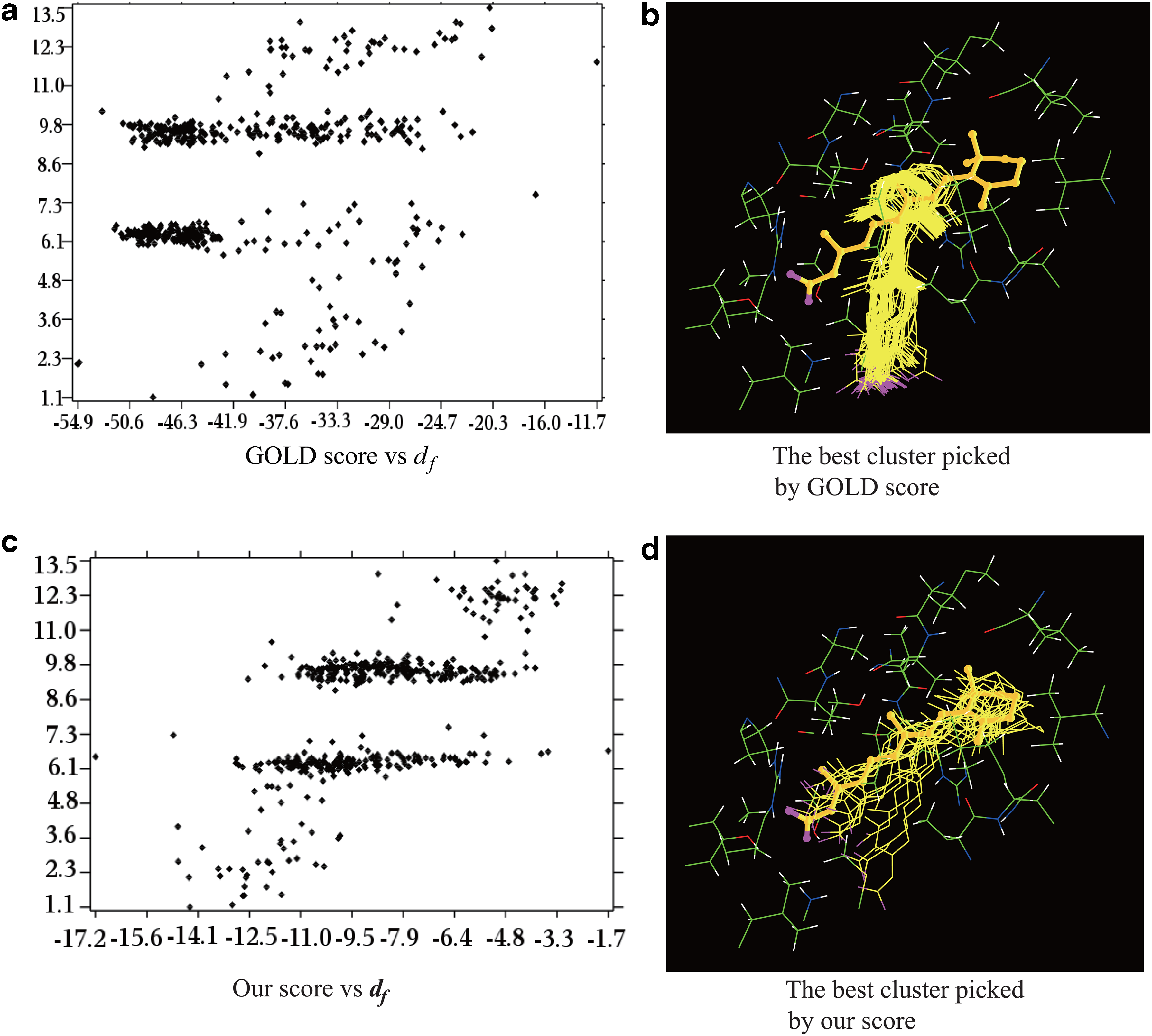
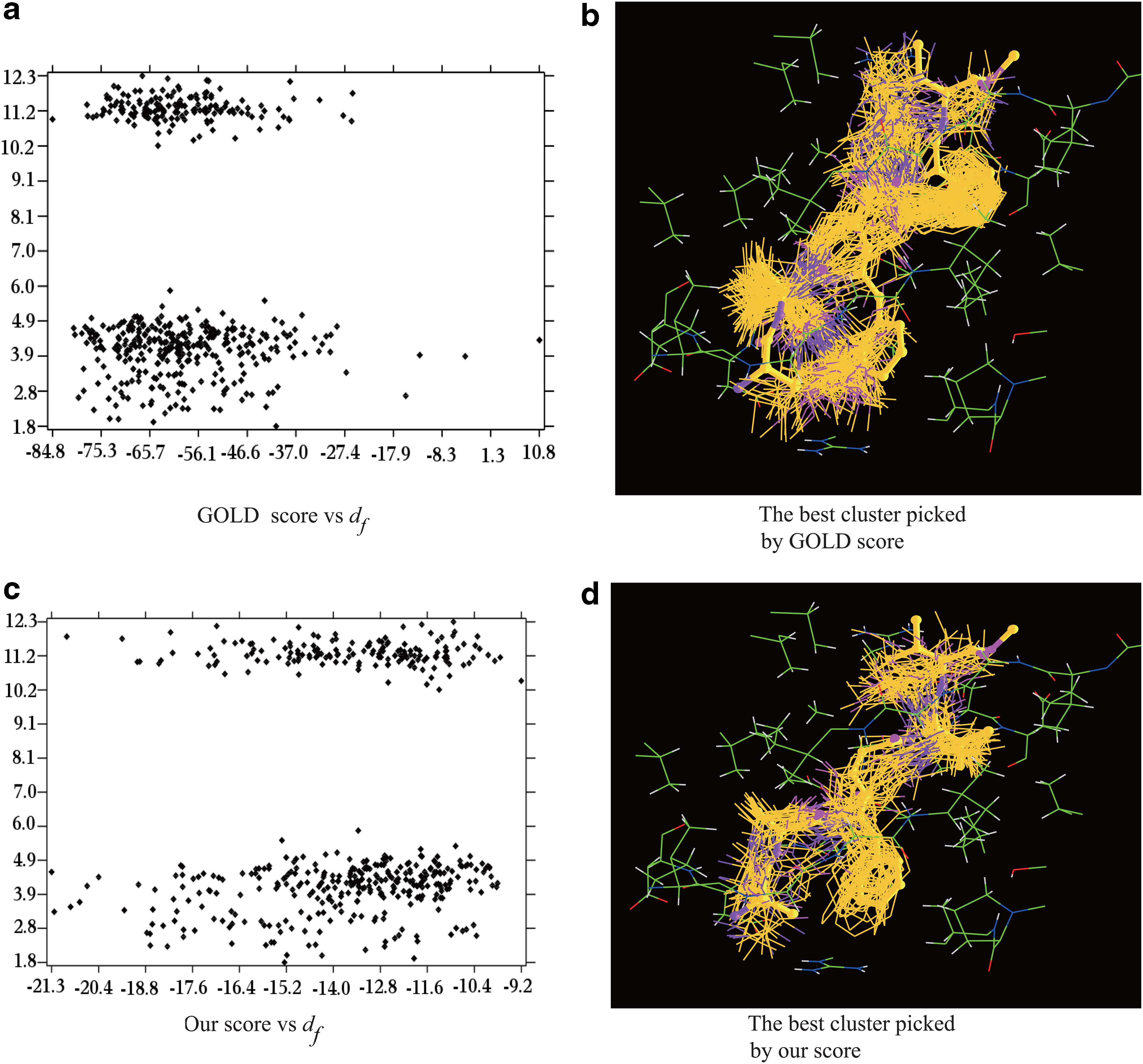
A comparison of GOLD and our scoring functions for best cluster selection for 1CBS. The x-axis and y-axis in (a, c) are respectively the score and d_f, the RMSD between the docked poses and experimental pose. GOLD ranks 82nd the pose with the smallest d_f while our score ranks it to the fifth. The lower a score, the better. The clusters in (b, d) are generated using the geometric algorithm with d_max=3.0Å. The protein atoms C, O, N, and H in the binding site are colored respectively in green, red, blue and white, while the C and O atoms of the ligand are colored in yellow and magenta. The experimental pose is depicted in a stick-and-ball model. The figures are prepared using our own molecule visualization program.

FIG. 2.

The comparison of GOLD vs our scoring function for best cluster selection for 1AAQ. The x-axis and y-axis in (a, c) are respectively the score and d_f. GOLD ranks 46 the pose with the smallest RMSD while our score ranks 188th. The protein, ligand and the poses are depicted and their atoms are colored in the same manner as in Fig. 1. The figures are prepared using our molecule visualization program.

The first example is human CRABP2 complexed with an RA analog (1CBS). We first generate three sets of clusters with decreasing d_max values (d_max=5.0Å, 4.0Å, 3.0Å), the average scores are then computed for each cluster (Table 2). Smaller d_max generates smaller but more accurate clusters. With d_max=5.0Å, there are four major clusters, while the poses in each of them distribute rather uniformly (Fig. 1a and c). Both GOLD and our scores could correctly select the most populated cluster as the best cluster. However, with d_max=4.0Å, GOLD picks wrongly the third cluster as the best one while our score identifies correctly the second one. With d_max=3.0, GOLD still selects the wrong cluster (the third cluster with 91 poses) (Fig. 1b) while our score identifies correctly the sixth cluster (15 poses) as the best one, with d_f=2.2Å (Fig. 1d). The main reason for the failure of the GOLD scoring function is that it does not include any term that accounts for the contribution of the intermolecular electrostatic interactions to the binding affinity. For CRABP2, it is well known that the electrostatic interaction between the carboxylic group of the RA analog and the two arginine residues (R111 and R132) contributes greatly to the binding (Wang et al., 1997).

Table 2.

Gold Score vs Our Score of the Most Populated Clusters for 1CBS Poses

d_max = 5.0Å
N_s	186	160	51	45
S_T	−10.0	−9.5	−6.5	−5.3
S_G	−44.1	−43.0	−35.5	−31.3
d_f	6.3	9.6	9.5	12.2

d_max = 4.0Å
N_s	160	126	91	45	25	18	6
S_T	−9.5	−10.5	−10.0	−5.3	−6.5	−6.7	−5.7
S_G	−43.0	−41.9	−45.4	−31.3	−4.7	−37.7	−33.7
d_f	9.6	5.3	6.2	12.2	9.5	9.5	9.5

d_max = 3.0Å
N_s	158	106	91	20	17	15	10	8	7	6
S_T	−9.4	−10.2	−10.0	−6.5	−5.0	−12.5	−6.8	−6.5	−5.3	−6.1
S_G	−43.1	−42.9	−45.4	−34.8	−30.6	−36.5	−37.6	−37.9	−31.6	−28.1
d_f	9.6	5.8	6.2	9.5	12.4	2.2	9.3	9.7	12.3	12.4

The clusters are generated using three decreasing d_maxs. The listed clusters include more than 90% of the total poses. N_s, S_T, S_G, and d_f are respectively the number of structures in a cluster, the average score computed using our and GOLD scoring functions, and the average RMSD between the GOLD generated poses and the experimental pose. The lower a score, the better. The three columns with the boldfaced numbers have the lowest average score as computed by our scoring function. RMSD, root-mean-square deviation.

The second example is an HIV protease complexed with a peptide analog (1AAQ). We first generate three sets of clusters with decreasing d_max values (d_max=4.5Å, 3.5Å, 3.0Å), and the average scores are then computed for each cluster (Table 3). We start with d_max=4.5Å, since only a single large cluster is generated with d_max=5.0Å. With d_max=4.5Å, there are four major clusters while the poses in each of them distribute very uniformly (Fig. 2a and c). GOLD wrongly picks the third cluster as the best one while our score identifies the second as the best, though the most populated one has slightly smaller d_f. With d_max=3.5Å, GOLD still picks wrongly the third (76 poses) as the best (Fig. 2b) while our score identifies the 4th (47 poses) (Fig. 2d), 5th (33 poses), and 7th (11 poses) clusters as the best ones with respective d_f of 2.7Å, 3.5Å, and 11.5Å. With d_max=3.0Å, GOLD again selects the wrong cluster (the 15th cluster with 5 poses) as the best, while our score identifies correctly the 14th cluster (6 poses) as the best, with d_f=2.1Å. For the HIV protease, the exclusion of electrostatic interaction in the GOLD scoring function may still contribute to its failure though the latter likely plays a small role. Though our scoring function outperforms the GOLD function in all the 22 cases tested it remains challenging for our function to select the correct cluster with 100% confidence. In this case, a dozen outliers with very low electrostatic energy or ligand internal energy must be removed, otherwise, with small d_max, both our and GOLD score may mistake the wrong clusters as the best ones. A systematic approach for outlier detection and for minimizing their ill-effects are under development.

Table 3.

Gold Score vs Our Score of the Most Populated Clusters for 1AAQ Poses

d_max = 4.5Å
N_s	179	131	80	52
S_T	−13.3	−13.6	−12.8	−13.5
S_G	−59.1	−58.8	−61.7	58.5
d_f (Å)	3.8	4.3	11.2	11.2

d_max = 3.5Å
N_s	127	91	76	49	33	31	11	10
S_T	−12.8	−13.1	−12.7	−14.7	−14.7	−13.1	−14.7	−14.3
S_G	−58.7	−58.8	−61.8	−59.7	−59.3	−58.6	−59.9	−59.0
d_f	4.2	4.6	11.2	2.7	3.5	11.2	11.3	11.5

d_max = 3.0Å
N_s	115	81	20	19	15	14	11	10	8
S_T	−12.7	−13.1	−12.7	−13.0	−13.8	−11.8	−14.5	−11.9	−13.7
S_G	−59.3	−58.9	−62.5	−62.9	−57.6	−63.1	−55.9	−61.1	−60.7
d_f	4.2	4.6	11.2	11.4	3.7	11.0	11.0	11.1	2.5

d_max = 3.0Å
N_s	7	6	6	6	6
S_T	−12.9	−14.2	−14.9	−15.1	−15.5
S_G	−58.6	−53.6	−53.4	−62.2	−62.4
d_f	11.1	11.0	2.4	11.2	2.1

The clusters are generated using three decreasing d_maxs. With d_max = 3.0Å the clusters whose number of poses is ≤1.0% of the total number of poses are not shown. The listed clusters include more than 85% of the total. The symbols have the same meanings as those in Table 2.

The complexity of the scoring functions forces almost all of the current docking programs to rely on heuristics for optimization. However, a heuristic search may not cover the pose space adequately, as being demonstrated in the above two examples; the poses with small d_f to the experimental one are the minority: accounting for less than 5% of the total poses. Another noticeable feature of the set of poses generated by GOLD is that the poses inside the first few largest clusters have similar GOLD scores though their d_f values differ greatly. Their large variations in d_f contribute to the improper ranking of the best clusters by the GOLD scoring function. In contrast, the combination of our scoring function with the geometric algorithm that is capable of classifying both uniformly and nonuniformly distributed data is capable of singling out the best clusters. In other words, the geometric clustering algorithm is ideally suitable for the identification of these minor clusters populated with the best poses.

4. Algorithmic Comparison

In this section, we first describe the six data sets used widely for the performance evaluation of clustering algorithms. Then we compare our algorithm with previous five algorithms from both theoretical and practical perspectives.

4.1. The test data sets

The six test data sets (Fig. 3) are generated using the statistical language R and a machine learning benchmark database program mlbench (Leisch and Dimitriadou, 2010; Newman et al., (1998). They are, respectively, two sets of uniformly distributed points over a 2D cube (a) and a 3D cube (b), a set of 3D points drawn from the spherical Gaussian distributions at the corners of a 3D unit hypercube (c), a set of points distributed over a 2D surface (a smiling face) (d), a set of 2D points (e) and a set of 3D points (f) drawn from two Gaussian distributions, each with a unit covariance matrix. Each data set has 1,000 points in total. The evaluation of the geometric algorithm and the comparisons with three previous clustering algorithms (nearest-neighbor, complete-link, and bipartition) that share with our algorithm the same classification criterion proceed as follows. Starting with 0.0, d_max is increased evenly by 0.1 at each step until it reaches an upper limit, and with each d_max the number of clusters generated by each algorithm is recorded (see Fig. 4). As one could tell easily from the Figure (Fig. 4), the geometric algorithm performs as well as complete-link and bipartition and is superior to the nearest-neighbor and biparition in terms of the number of clusters generated per d_max value. In addition, the geometric algorithms runs more efficiently than either bipartition or complete-link algorithm.

FIG. 3.

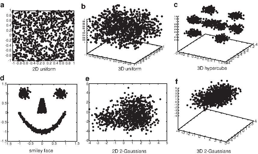
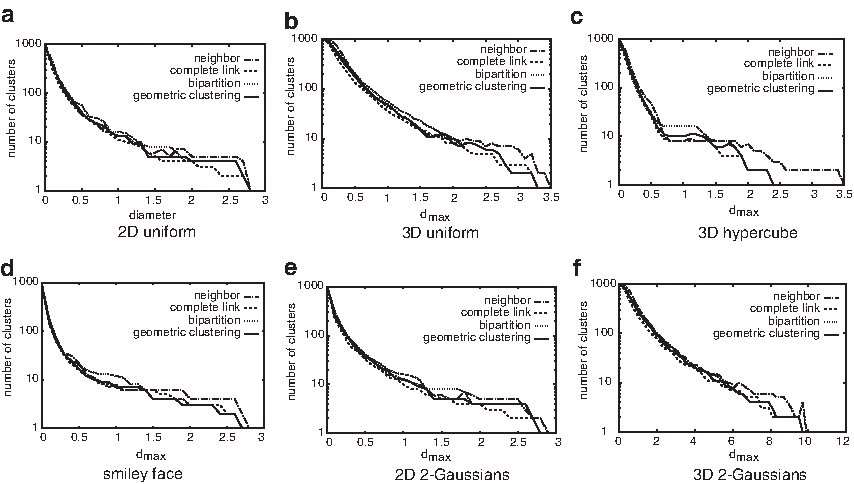
The six test data sets. (a) A set of uniformly distributed points over a 2D cube, (b) a set of uniformly distributed points over a 3D cube, (c) a set of 3D points drawn from the spherical Gaussian distributions at the corners of a 3D unit hypercube; (d) a set of points distributed over a 2D plane surface (a smiling face), (e) a set of 2D points from two Gaussian distributions each with a unit covariance matrix, and (f) a set of 3D points from two Gaussian distributions, each with a unit covariance matrix.

FIG. 4.

A comparison of our algorithm with the nearest-neighbor, complete-link, and bipartition algorithms on the six test data sets. The x-axis is d_max; the y-axis is the corresponding number of clusters (shown in log scale).

4.2. Algorithmic comparison

Data classification by means of clustering is a natural exploratory process for knowledge discovery, and thus clustering algorithms have found wide applications in many different areas. The clustering algorithms themselves could be classified into two groups based on their goals. Those in the first group (e.g., k-medoids and average-link) share the goal to minimize the metrics (e.g., the metric to the center of the cluster) of all the data points assigned to the same cluster, while those in the second group aim to minimize the number of clusters and simultaneously to satisfy the classification criterion that any pairwise metric in a cluster is less than a certain value. Our algorithm belongs to the second group as are the nearest-neighbor, bipartition, and complete-link algorithms. In our algorithm the seeds for new clusters are those data points that form the largest polyhedron. These points are likely to be labeled as “outliers” by the algorithms of the first group, but our algorithm initializes the clustering process with them and thus ensures them and together with their neighbors to be in different clusters.

Consequently, the representatives of the clusters from our algorithm sample the data space more uniformly than those from an average-link algorithm and much more uniformly than those from a k-medoid do. The geometric algorithm, differs largely from k-mean or k-medoid algorithms, and thus have no problems associated with them such as (a) the tendency to find hyperspherical clusters, (b) the danger of falling into local minimal, and (c) the variability in results that depends on the choice of the initial seeds. Because our algorithm classifies the data by iteratively separating them into smaller clusters according to their distances to the seeds, it will not be affected by an irregular or nonuniform distribution, as it is for a density-based clustering algorithm such as the k-medoids. The results from the applications to the clustering of both the intermediate structures and poses suggest that the k-medoids algorithm are not suitable for structural data classification.

The geometric algorithm shares some critical features with the other algorithms in the second group. However, unlike a hierarchical algorithm such as the complete-link that only optimizes an objective function locally, our algorithm takes into consideration the global information in the very beginning. The average time complexity of our algorithm is O(n² log n) that is the same as the complexity of the agglomerative hierarchical algorithm implemented with a priority queue Day and Edelsbrunner (1984). Furthermore, the implementation suggests that our algorithm is faster than the hierarchical algorithms, most likely because the base in the logarithmic function is ≥4 rather than 2 as in a typical hierarchical algorithm. In a sense, the geometric algorithm could be looked upon as an extension of a bipartition algorithm except that the geometric algorithm may use up to any number of seed points at each step while a bipartition algorithm could use only two. An algorithm runs faster with more seeds at each step.

The geometric algorithm is somewhat similar to the minimum-diameter divisive hierarchical algorithm by (Guenoche et al., 1991). The key difference lies in how a previous cluster is divided into new clusters: in the minimum-diameter hierarchical algorithm, two new clusters are generated by an expensive search for the two balls with the minimum diameters while in our algorithm up to four new clusters are initialized with the seeds computed in linear time in terms of the number of data points in the previous cluster. In summary, the applications to both real structural data and test data have demonstrated that the performance of our algorithm is either similar to or better than that of a nearest-neighbor, bipartition, or complete-link algorithm. A possible drawback of our algorithm as well as the other algorithms in the second group is that prior knowledge is required to specify a d_max value, and several d_max values may need to be tried in order to find the best classification for a data set. As far as the structural data is concerned, it is not difficult for the practitioners to find a reasonable d_max based on the quality of the data or the required precision in the final clusters.

5. The Challenges Of Structural Data Classification

Though at present many clustering algorithms are available, as shown by Kleinberg (2002), there exists no best or universal clustering algorithm that could be applied to any type of data with equal success. The classification of structural data, especially those computed using restraints, poses particular challenges because one must take into consideration their unique features, such as the distribution of data may be both uniform and nonuniform or both regular and irregular because of the sparseness of the input restraints, the errors in the scoring function, the limited sampling provided by heuristics, and the extreme energy level degeneracy of biomolecules in solution (Landau and Lifshitz, 1980). The lack of a solid theoretical foundation for a general clustering algorithm and the difficulty in structural data clustering have led to quite some confusion about the classification of the protein global folds in the PDB (Orengo et al., 1997; Murzin et al., 1995) and make it rather tricky to compare different protein active sites. An objective classification of global folds and active sites should be based solely on a structural clustering algorithm without any manual intervention. Though, as shown in the article the geometric algorithm is both efficient and more suitable than the previous algorithms for structural data classification, much efforts are required for the design of a robust clustering algorithm with a solid theoretical foundation that could be relied on for the objective classification of global folds, active sites, and ligand poses.

Footnotes

Author Disclosure Statement

The authors declare that no competing financial interests exist.

References

Adzhubei

A.A.

, Laughton

C.A.

, and Neidle

1995. An approach to protein homology modelling based on an ensemble of NMR structures: application to the Sox-5 HMG-box protein. Protein Eng., 8, 615–625.

Baker

N.A.

, Sept

, Joseph

, et al. 2001. Electrostatics of nanosystems: Application to microtubules and the ribosome. PNAS, 98, 10037–10041.

Blumenthal

L.M.

1970. Theory and applications of distance geometry. Chelsea Publishing, New York.

Bottegoni

, Rocchia

, and Cavalli

2012. Application of conformational clustering in protein–ligand docking, 169–186. In Walker

J.M.

, ed., Computational Drug Discovery and Design. Humana Press, New York.

Day

W.H.E.

, and Edelsbrunner

1984. Efficient algorithms for agglomerative hierarchical clustering methods. J. Classif., 1, 7–24.

Domingues

F.S.

, Rahnenführer

, and Lengauer

2004. Automated clustering of ensembles of alternative models in protein structure databases. Protein Eng. Des. Sel., 17, 537–543.

Downs

G.M.

, and Barnard

J.M.

2002. Clustering methods and their uses in computational chemistry. Rev. Comput. Chem., 18, 1–40.

Guenoche

, Hansen

, and Jaumard

1991. Efficient algorithms for divisive hierarchical clustering with the diameter criterion. J. Classif., 8, 5–30.

Jain

A.K.

, Murty

M.N.

, and Flynn

P.J.

1999. Data clustering: a review. ACM Comput. Surv., 31, 264–323.

10.

Jain

A.K.

2010. Data clustering: 50 years beyond k-means. Pattern Recogn. Lett., 31, 651–666.

11.

Jones

, Willett

and Glen

R.C.

1995. Molecular recognition of receptor sites using a genetic algorithm with a description of desolvation. J. Mol. Biol., 245, 43–53.

12.

Keller

, Daura

, and Gunsteren

W.F.

2010. Comparing geometric and kinetic cluster algorithms for molecular simulation data. J. Chem. Phys., 132, 074110

13.

Kleinberg

J.M.

2002. An impossibility theorem for clustering. Advances in Neural Information Processing Systems 15, NIPS, 2002, 463–470.

14.

Landau

L.D.

, and Lifshitz

E.M.

1980. Statistical Physics, Vol. 5. Pergamon Press, Oxford.

15.

Leisch

, and Dimitriadou

2010. mlbench: Machine Learning Benchmark Problems. R package version 2.1-1. Available at: http://cran.r-project.org Accessed October 2013 .

16.

Lloyd

S.P.

1982. Least squares quantization in PCM. IEEE Trans. Inf. Theory, 28, 129–136.

17.

May

A.C.W.

1999. Toward more meaningful hierarchical classification of protein three-dimensional structures. PROTEINS, 37, 20–29.

18.

Murzin

A.G.

, Brenner

S.E.

, Hubbard

, et al. 1995. Scop: A structural classification of proteins database for the investigation of sequences and structures. J. Mol. Biol., 247, 536–540.

19.

Newman

D.J.

, Hettich

, Blake

C.L.

, et al. 1998. Uci repository of machine learning databases. Available at: www.ics.uci.edu Accessed October 2013 .

20.

Orengo

C.A.

, Michie

A.D.

, Jones

, et al. 1997. Cath–A hierarchic classification of protein domain structures. Structure, 5, 1093–1108.

21.

Sadowski

, Gasteiger

, and Klebe

1994. Comparison of automatic three-dimensional model builders using 639 x-ray structures. J. Chem. Inf. Comput. Sci., 34, 1000–1008.

22.

Shao

, Tanner

S.W.

, Thompson

, et al. 2007. Clustering molecular dynamics trajectories: 1. characterizing the performance of different clustering algorithms. J. Chem. Theory Comput., 3, 2312–2334,

23.

Sutcliffe

M.J.

1993. Representing an ensemble of nmr-derived protein structures by a single structure. Protein Sci., 2, 936–944.

24.

Wang

, Mettu

, and Donald

B.R.

2006. A polynomial-time algorithm for de novo protein backbone structure determination from NMR data. J. Comput. Biol., 13, 1276–1288.

25.

Wang

, Li

, and Yan

1997. Structure-function relationships of cellular retinoic acid-binding proteins: Quantitative analysis of the ligand binding properties of the wild-type proteins and site-directed mutants. Biol. Chem., 272, 1541–1547.

26.

Warren

G.L.

, Andrews

C.W.

, Capelli

A.M.

, et al. 2006. A critical assessment of docking programs and scoring functions. J. Med. Chem., 49, 5912–5931.

Supplementary Material

Please find the following supplemental material available below.

For Open Access articles published under a Creative Commons License, all supplemental material carries the same license as the article it is associated with.

For non-Open Access articles published, all supplemental material carries a non-exclusive license, and permission requests for re-use of supplemental material or any part of supplemental material shall be sent directly to the copyright owner as specified in the copyright notice associated with the article.

0.00 MB

0.08 MB

A Geometric Clustering Algorithm with Applications to Structural Data

Abstract

Abstract

1. Introduction

2. The Algorithm and Data Set

2.1. The geometric partitional algorithm

2.2. Running time

2.3. Structural data set

2.3.1. NMR data set

2.3.2. The set of poses from protein-ligand docking

3. Results and Discussion

3.1. NMR structural ensemble

3.2. Protein-ligand docking

4. Algorithmic Comparison

4.1. The test data sets

4.2. Algorithmic comparison

5. The Challenges Of Structural Data Classification

Footnotes

Author Disclosure Statement

References

Supplementary Material