
Abstract
Abstract
Among the methods currently available for inferring species trees from gene trees, the GLASS method of Mossel and Roch (2010), the Shallowest Divergence (SD) method of Maddison and Knowles (2006), the STEAC method of Liu et al. (2009), and a related method that we call Minimum Average Coalescence (MAC) are computationally efficient and provide branch length estimates. Further, GLASS and STEAC have been shown to be consistent estimators of tree topology under a multispecies coalescent model. However, divergence time estimates obtained with these methods are all systematically biased under the model because the pairwise interspecific gene divergence times on which they rely must be more ancient than the species divergence time. Jewett and Rosenberg (2012) derived an expression for the bias of GLASS and used it to propose an improved method that they termed iGLASS. Here, we derive the biases of SD, STEAC, and MAC, and we propose improved analogues of these methods that we call iSD, iSTEAC, and iMAC. We conduct simulations to compare the performance of these methods with their original counterparts and with GLASS and iGLASS, finding that each of them decreases the bias and mean squared error of pairwise divergence time estimates. The new methods can therefore contribute to improvements in the estimation of species trees from information on gene trees.
1. Introduction
GLASS, SD, and STEAC are all distance-matrix methods. Such methods first estimate an evolutionary distance between each pair of taxa and then construct a species tree that provides an approximate representation of the pairwise distances. In GLASS, SD, and STEAC, divergence times are estimated for each pair of species, and a hierarchical clustering method is then applied to the pairwise distances to construct an estimate of the species tree. Thus, each distance-matrix method can be viewed as an estimator of pairwise species divergence times combined with a hierarchical clustering procedure.
To understand the general approach by which GLASS, SD, and STEAC estimate the divergence time between a pair of taxa A and B, consider a set of L loci indexed by ℓ, and denote by
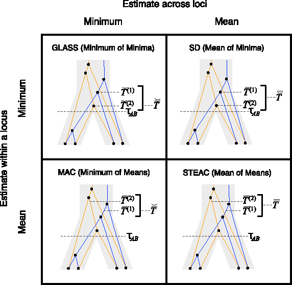
Four methods for estimating divergence times from sets of multiple lineages sampled at many loci in two species. The same species tree and gene trees are pictured in all four panels. In the first row, we consider
The GLASS, SD, and STEAC estimation methods each consider a minimum or mean of either the
The species divergence time estimates given by GLASS, SD, STEAC, and MAC are all systematically biased under the multispecies coalescent, a basic evolutionary model for describing the evolution of gene trees conditional on species trees (Degnan and Rosenberg, 2009). This bias arises because, under the model, true pairwise interspecific gene coalescence times
For the GLASS method, Jewett and Rosenberg (2012) addressed the issue of bias by proposing an improved method for estimating pairwise divergence times. This method, which they called iGLASS, adjusts the GLASS estimate downward by an amount related to the bias of GLASS. Jewett and Rosenberg showed that iGLASS is consistent for estimating pairwise divergence times and that it can be combined with a suitable clustering algorithm to produce a consistent estimator of the species tree topology. Through simulations, they found that iGLASS greatly reduces the bias and mean squared error of pairwise divergence time estimates produced by GLASS.
Here, we propose improved analogues for SD, STEAC, and MAC, which we call iSD, iSTEAC, and iMAC, respectively, under which bias in the estimation of species divergence times is substantially reduced or eliminated. In Section 2, we derive the improved methods for estimating pairwise divergence times. Our derivations first quantify the bias in pairwise estimates of species divergence time for each of the original three methods as a function of the true divergence time, the number of lineages sampled from each taxon, and the number of sampled loci. Given a divergence time estimate obtained using one of the original methods, an improved estimate is produced by subtracting from the original estimate its bias; more precisely, because the bias for a given scenario depends on the true divergence time, which we are attempting to estimate, we calculate improved estimates by solving an equation for the true divergence time that will be detailed in Section 2. In Section 3, we evaluate the methods for estimating pairwise divergence times, and we compare the performance of the improved methods with each other and with their original counterparts. We also expand the analysis to trees with more than two taxa; in these cases, the improved version of a given method (GLASS, SD, STEAC, or MAC) is obtained by calculating the improved pairwise divergence time estimate for each pair of taxa and then applying a clustering method to the matrix of improved estimates. We compare the original and improved methods for inferring these larger trees with respect to both the bias and mean squared error in pairwise divergence time estimates and the proportion of sampled trees for which the correct topology is inferred.
2. Derivation Of Improved Methods
We follow the assumptions of a simple multispecies coalescent model (Degnan and Rosenberg, 2009). Each branch i of the species tree is assumed to have a constant effective population size Ni. Looking backward in time from the present at a species tree branch with n sampled lineages, we assume that all
Bias reduction is carried out in a similar way for each of the four estimators that we consider. As we have discussed, Jewett and Rosenberg (2012) examined the bias reduction in the case of GLASS; here, we proceed more generally. Consider a specific estimator tAB chosen from among the four in our study; that is, tAB represents either
for τ AB .
In the case in which the estimate
The improved estimate for the pairwise species divergence time,
As we will see, except in the case of STEAC, this procedure gives an estimate of τ AB that is biased when more than one lineage is sampled in each taxon. However, the bias of each improved estimator is greatly reduced compared to that of the corresponding original estimator.
To simplify our derivations, we define a random variable VAB as the difference between the estimator tAB and the true speciation time τ
AB
; that is, VAB = tAB − τ
AB
. VAB measures the extent to which a random estimate exceeds the true speciation time. We can now express
2.1. Glass
As derived by Jewett and Rosenberg (2012), the iGLASS estimator can be obtained by first deriving
2.1.1. Derivation of
\documentclass{aastex}\usepackage{amsbsy}\usepackage{amsfonts}\usepackage{amssymb}\usepackage{bm}\usepackage{mathrsfs}\usepackage{pifont}\usepackage{stmaryrd}\usepackage{textcomp}\usepackage{portland, xspace}\usepackage{amsmath, amsxtra}\pagestyle{empty}\DeclareMathSizes{10}{9}{7}{6}\begin{document}
$$E_{\tau_{AB}} [\check{\check{V}}_{AB}]$$
\end{document}
for a single locus
Define
where
with
The density
where
Here,
2.1.2. Derivation of
\documentclass{aastex}\usepackage{amsbsy}\usepackage{amsfonts}\usepackage{amssymb}\usepackage{bm}\usepackage{mathrsfs}\usepackage{pifont}\usepackage{stmaryrd}\usepackage{textcomp}\usepackage{portland, xspace}\usepackage{amsmath, amsxtra}\pagestyle{empty}\DeclareMathSizes{10}{9}{7}{6}\begin{document}
$$E_{\tau_{AB}} [\check{\check{V}}_{AB}]$$
\end{document}
for multiple loci
To derive the iGLASS correction for multiple loci, Jewett and Rosenberg (2012) obtained the conditional expectation,
The unconditional expectation
2.2. SD
2.2.1. Derivation of
\documentclass{aastex}\usepackage{amsbsy}\usepackage{amsfonts}\usepackage{amssymb}\usepackage{bm}\usepackage{mathrsfs}\usepackage{pifont}\usepackage{stmaryrd}\usepackage{textcomp}\usepackage{portland, xspace}\usepackage{amsmath, amsxtra}\pagestyle{empty}\DeclareMathSizes{10}{9}{7}{6}\begin{document}
$$E_{\tau_{AB}} [\bar{\check{V}}_{AB}]$$
\end{document}
for a single locus
The SD estimator,
2.2.2. Derivation of
\documentclass{aastex}\usepackage{amsbsy}\usepackage{amsfonts}\usepackage{amssymb}\usepackage{bm}\usepackage{mathrsfs}\usepackage{pifont}\usepackage{stmaryrd}\usepackage{textcomp}\usepackage{portland, xspace}\usepackage{amsmath, amsxtra}\pagestyle{empty}\DeclareMathSizes{10}{9}{7}{6}\begin{document}
$$E_{\tau_{AB}} [\bar{\check{V}}_{AB}^{(\ell)}]$$
\end{document}
for multiple loci
For a set of L loci, we take the mean of
Similarly to the procedure for GLASS, the expectation from (9) is then inserted into Equation (2), which is then solved for
2.3. MAC
2.3.1. Derivation of
\documentclass{aastex}\usepackage{amsbsy}\usepackage{amsfonts}\usepackage{amssymb}\usepackage{bm}\usepackage{mathrsfs}\usepackage{pifont}\usepackage{stmaryrd}\usepackage{textcomp}\usepackage{portland, xspace}\usepackage{amsmath, amsxtra}\pagestyle{empty}\DeclareMathSizes{10}{9}{7}{6}\begin{document}
$$E_{\tau_{AB}} [\check{\bar{V}}_{AB}]$$
\end{document}
for a single locus
To obtain the iMAC estimator, we begin by deriving the distribution of
Because many gene tree topologies are possible when more than one lineage is sampled from each taxon, we further condition on a certain set of unlabeled tree topologies,
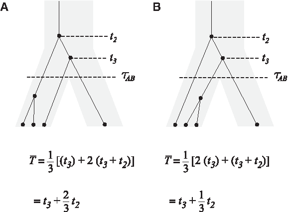
Two trees with identical topologies above the root, but different mean interspecific coalescence times. As in Section 2.3, ti denotes the waiting time until i lineages coalesce to i − 1 lineages.
Given
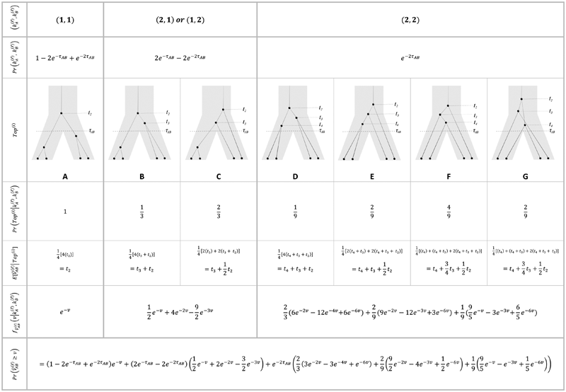
The set of distinct topologies, pictured in the third row, is formed by considering the
Conditional on tree topology, we calculate the density of
For a more complex example, consider Table 1F. Here, the first of the four pairwise interspecific coalescences occurs at the first coalescent event past divergence, when four lineages remain; we denote the waiting time until this coalescence by t4. The second pairwise interspecific coalescence occurs at the next coalescent event, so that the waiting time past the divergence for this coalescent event is t4 + t3. Finally, the last two pairwise interspecific coalescences, between the rightmost lineage and each of the two lineages of the left taxon, occur at the last coalescent event, which occurs at time t4 + t3 + t2 past the divergence time. The mean, as given in the figure, is therefore
In this equation (Ross, 2007), independent exponential random variables are denoted
Once
With the conditional densities of
We then find the distribution of
where we define the starting point of the summation for
2.3.2. Derivation of
\documentclass{aastex}\usepackage{amsbsy}\usepackage{amsfonts}\usepackage{amssymb}\usepackage{bm}\usepackage{mathrsfs}\usepackage{pifont}\usepackage{stmaryrd}\usepackage{textcomp}\usepackage{portland, xspace}\usepackage{amsmath, amsxtra}\pagestyle{empty}\DeclareMathSizes{10}{9}{7}{6}\begin{document}
$$E_{\tau_{AB}} [\check{\bar{V}}_{AB}]$$
\end{document}
for multiple loci
For one locus, the probability that
For many loci, the survival function of
In the case in which the same numbers of lineages are sampled at each locus, the survival functions for different loci are identical, and Equation (14) further simplifies to
The expectation required in computing the iMAC estimator can then be found by integration:
Equation (16) gives the expectation that is inserted into Equation (2) to obtain the iMAC estimate according to Equation (3).
2.4. STEAC
The STEAC estimator of Liu et al. (2009) is found by computing the mean pairwise interspecific coalescence time for each locus, and then taking the mean of these times over all loci. Because the expected time until two lineages from different taxa coalesce is one coalescent unit past the divergence time, or
3. Comparison Of Methods
3.1. Bias and mean squared error in pairwise divergence time estimates
Each of the four improved methods has the potential to substantially reduce bias in estimates of species divergence times. Some bias remains in the improved estimates, however, and we use simulations to examine bias and mean squared error (MSE) for all of the methods.
3.1.1. Simulation procedure
We performed simulations using the multispecies coalescent model, following a procedure similar to that of Jewett and Rosenberg (2012). Briefly, in each daughter branch with n sampled lineages, two lineages were chosen randomly to coalesce, with coalescence time following an exponential distribution with mean
We considered several simulated scenarios, with true divergence times set to 0, 0.1, 0.3, 0.6, 1.0, 1.5, 2.1, 2.8, and 3.6 coalescent units and with the number of loci varied from 1 to 10 in unit increments. These divergence times and numbers of loci were chosen so that trends in each parameter, as well as differences among the methods over a biologically realistic range, could potentially be detected. Simulations for each of the eight methods (GLASS, iGLASS, SD, iSD, MAC, iMAC, STEAC, and iSTEAC) were performed separately. For each method, we simulated a set of 50,000 replicate experiments for each of the 90 combinations of divergence time and number of loci, with two lineages sampled from each taxon. Two lineages were sampled for the small-sample-size simulations because with a single sampled lineage, the mean pairwise interspecific coalescence and the minimum pairwise interspecific coalescence are equivalent; differences between GLASS and MAC and between SD and STEAC would then be undetectable. To investigate sample-size effects, simulations were repeated with four lineages sampled per taxon. For these larger-sample-size simulations, the number of sampled lineages was limited to four because it is desirable to compare all methods at the same sample size, and computing the distributions of the mean pairwise interspecific coalescence times necessary for evaluation of iMAC was prohibitive with larger sample sizes.
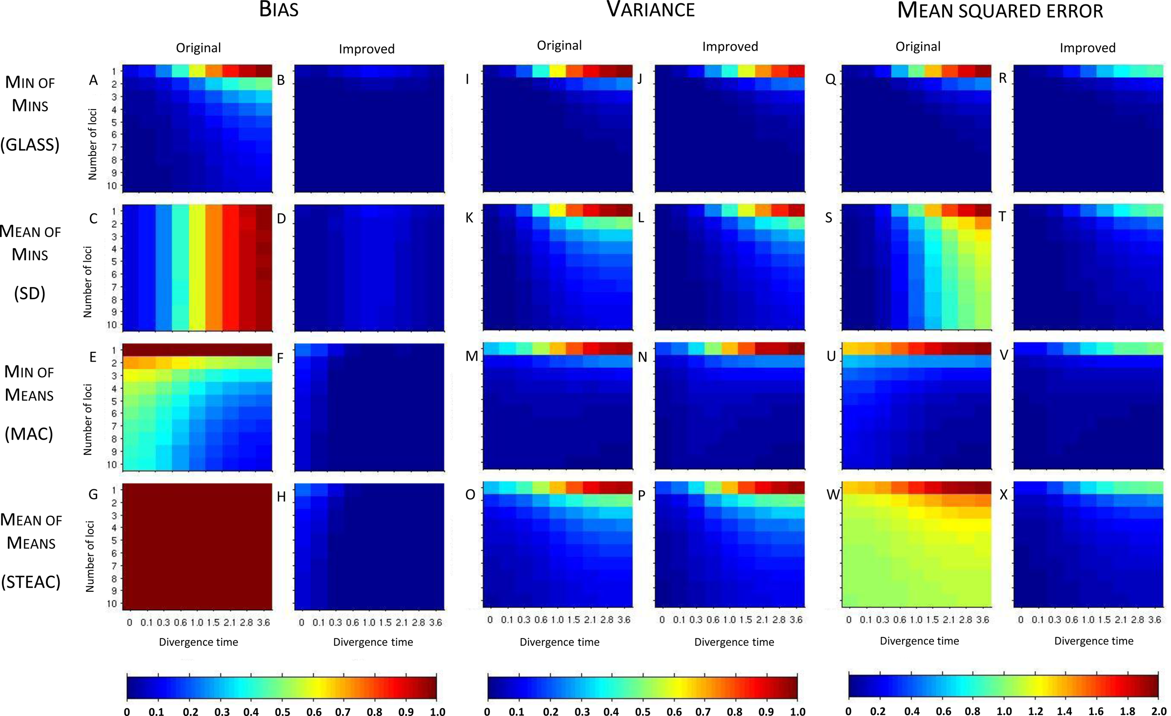
Figure 3 shows the resulting bias, variance, and MSE in the 50,000 simulations for each of the four pairs of original and improved methods, for each of the 90 combinations of divergence time and number of loci, with two lineages sampled from each taxon. Figure 4 shows corresponding results for the case in which four lineages were sampled from each taxon.
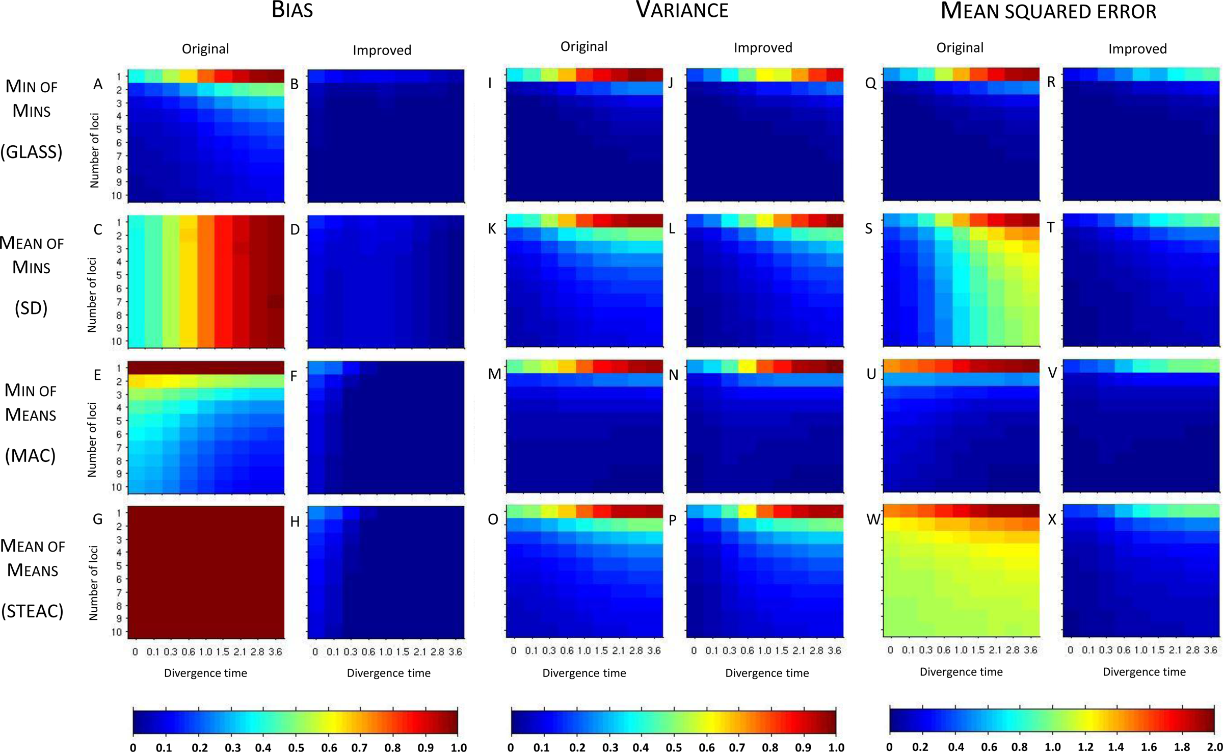
Bias, variance, and mean squared error in the estimation of divergence times for the original and improved STEAC, SD, MAC, and GLASS methods. Two taxa are considered, with two lineages sampled from each taxon at each locus. Estimates were evaluated at divergence times of 0, 0.1, 0.3, 0.6, 1.0, 1.5, 2.1, 2.8, and 3.6 coalescent units and with 1, 2, 3, 4, 5, 6, 7, 8, 9, and 10 loci. 50,000 replicates were generated separately for each scenario and each method.
Bias, variance, and mean squared error in the estimation of divergence times for the original and improved STEAC, SD, MAC, and GLASS methods, with a larger sample size than that pictured in Figure 3. Two taxa are considered, with four lineages sampled from each taxon at each locus. Estimates were evaluated at divergence times of 0, 0.1, 0.3, 0.6, 1.0, 1.5, 2.1, 2.8, and 3.6 coalescent units and with 1, 2, 3, 4, 5, 6, 7, 8, 9, and 10 loci. 50,000 replicates were generated separately for each scenario and each method.
3.1.2. Equivalences among special cases
In order to better analyze trends in the bias, variance, and MSE among the methods, we first highlight two special cases that produce equivalencies among some of our methods from shared features in the ways that the methods are constructed. First, suppose that only a single locus is sampled, as in the first rows of each heat map panel of Figure 3. Comparing the first rows of Figure 3A,C, we see that if a single locus is sampled, then GLASS and SD produce identical results. GLASS considers the minimum over loci of the locus-specific minimum coalescence times, while SD considers the mean over loci of the minimum coalescence times; for a single locus, the methods are equivalent. By the same logic, MAC, which considers the minimum over loci of locus-specific mean coalescence times, and STEAC, which considers the mean over loci of the locus-specific mean coalescence times, are also equivalent for a single locus; this result can be seen by comparing the first rows of the heat maps in Figure 3E,G. In the single-locus case, GLASS, SD, MAC, and STEAC are all identical when one lineage is sampled per taxon.
A second relationship can be seen by considering large divergence times, as shown in Figure 3 by the rightmost columns of the heat maps. As the divergence time becomes large, at any locus, the probability is high that only a single lineage will remain in each branch when the divergence time is reached. In this case, the mean and minimum interspecific coalescence at a given locus will be the same. Thus, GLASS and MAC are asymptotically equivalent at large divergence times, as are SD and STEAC. This result can be verified by comparing the rightmost columns of the heat maps in Figure 3A with those in Figure 3E, and those in Figure 3C to those in Figure 3G. At infinite divergence times in the case of a single locus, all four methods would be equivalent.
3.1.3. Bias
Considering the simulation results for the various methods individually, in Figure 3A we see that the original GLASS method has a relatively low bias compared with the other original methods (Fig. 3C,E,G). A notable improvement is still made by the approximate iGLASS method of Jewett and Rosenberg (2012), in Figure 3B, particularly when few loci are sampled and at high divergence times.
In Figure 3C, a striped pattern in the heat map for the SD method confirms that with divergence time held constant,
The bias of MAC is shown in Figure 3E. As mentioned in Section 2.4, we see that for a single locus, bias is constant at a value of one coalescent unit. For more than one locus, unlike for GLASS and SD, the bias of MAC is most pronounced for short divergence times. At short divergence times, the numbers of lineages remaining at the divergence time will be larger than when the divergence time is large, and the mean pairwise interspecific coalescence time will have a smaller variance around its expected value of one coalescent unit. With few loci, the minimum of these times across loci is still likely to be quite high. As we will see in the next section, larger divergence times or more sampled loci increase the probability that one of the mean pairwise interspecific coalescence times will be small; in such cases, the MAC estimator will be less biased. Even so, for the bias in the iMAC estimator, a considerable improvement is seen over MAC (Fig. 3F).
Figure 3G shows that the bias of STEAC is constant at one coalescent unit regardless of the divergence time or number of loci sampled, as shown in Section 2.4. A marked improvement in bias for iSTEAC compared with STEAC is shown in Figure 3H, where the bias is reduced to a maximum of about 0.26 coalescent units in the case of only one locus sampled and a divergence time of zero. Note that the bias of iSTEAC is not zero because the iSTEAC estimate is set to zero rather than a negative value whenever the unimproved STEAC estimate is smaller than its smallest expected value, leading to upwardly biased estimates.
Comparing the four improved methods in Figure 3B,D,F,H, we see that all four improved methods have bias of similar magnitude. Furthermore, for each improved method, bias decreases with increasing divergence time or number of loci, with slight exceptions in the iGLASS and iSD cases resulting from the use of the approximate correction. Some differences between methods are seen for shorter divergence times or fewer loci. For small divergence times, iGLASS has the lowest bias for all of the numbers of loci that we have considered. For intermediate and long divergence times and when only a single locus is considered, iMAC and iSTEAC provide the least-biased estimates. At intermediate and long divergence times and when more than one locus is considered, iGLASS, iMAC, and iSTEAC yield the lowest biases.
3.1.4. Variance
The variances in pairwise species divergence time estimates generated by the four original and four improved methods appear in Figures 3I–P. Each unimproved method shows a pattern of variance in which values are higher at large divergence times and small numbers of loci. For larger divergence times, it is likely that only one lineage will remain in each taxon at the divergence time, and the resulting coalescence time between these two lineages will have a higher variance than will the minimum or mean coalescence time between multiple lineages. The greater variance when fewer loci are sampled is a standard effect of sampling more data: estimates based on only a few locus-specific values will have higher variance than those based on more loci.
Little change in variance is seen between any original method and its improved analogue. This result can be explained by viewing our bias reduction process as being approximately equivalent to subtracting a constant from the original estimates, an adjustment that would leave the variance unchanged. The small changes in variance that do occur arise from two deviations between the actual bias reduction method and this simplified scenario. First, in solving Equation (3), except in the case of STEAC, the amount subtracted from an estimate
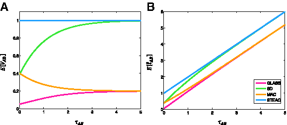
E[VAB] and
The four original methods have similar variances (Fig. 3I,K,M,O), and because variance changes little between the original and improved estimates, the improved methods also have similar variances (Fig. 3J,L,N,P). As in the case of the original methods, variances for the improved methods increase with increasing divergence times and decrease with increasing numbers of loci. Variance is lowest for iGLASS, followed by iMAC, then by iSD, and iSTEAC.
3.1.5. Mean squared error
Considered together, the bias and variance results explain the patterns seen in the mean squared error (MSE) of the divergence time estimates in Figure 3Q–X. The reduction in MSE from the original to the improved methods is mostly due to the decrease in bias. Comparing the four improved methods, in Figure 3R,T,V,X, we see that the MSE in the improved methods largely shows the same pattern as the variance, increasing with greater divergence times and decreasing with greater numbers of loci. For intermediate and large divergence times, iGLASS has the lowest MSE, followed by iMAC, iSD, and iSTEAC.
3.2. Sample size
To investigate the effect of sample size on the various estimation methods, we can compare Figure 4, which considers samples of size four from each species, with Figure 3, which considers samples of size two. The comparison shows that patterns in bias, MSE, and variance are similar between the two scenarios. For large divergence times, we expect the values to be identical because at large divergence times, the probability is high that only one lineage from each branch will survive until the divergence, regardless of the initial number of lineages sampled.
At small divergence times, a comparison of Figure 4A,C with Figure 3A,C shows that the original GLASS and SD methods have less bias as the number of sampled lineages increases. Because the minimum interspecific coalescent event is considered at each locus for these methods, and because we expect the first interspecific coalescent event to occur sooner after divergence when more lineages are available at the divergence time, this result is not surprising. For the MAC method in Figures 3E and 4E, particularly at small divergence times and when more than one locus is considered, we see an increase in the bias of the original method with increasing sample size. This increase occurs because the variance of the mean pairwise interspecific coalescence time at each locus decreases when more lineages are available at the divergence time to coalesce, reducing the probability that the mean pairwise interspecific coalescence time at a given locus will be near the divergence time. Figure 4G confirms that the bias in STEAC is constant with respect to sample size.
For the improved methods, slight decreases in bias are seen with increasing sample size. In Figure 3B,D,F,H, as noted above, the bias is greatest when divergence times are low. This result is due to the fact that in these cases, many estimates that lie below their expected value, and that would produce improved estimates that would underestimate the true divergence time, are set to zero by the procedure in Equation (3). The original estimates that exceed their expectations, however, still overestimate the true divergence time, and a positive bias is introduced. When sample size is increased, the variance of the original estimates decreases, as can be seen by comparing Figure 4I,K,M,O with Figure 3I,K,M,O; as a result of this decrease in variance, fewer estimates are set to zero at small divergence times, and the positive bias in the estimates is reduced. Thus, because SD experiences a relatively large reduction in variance with the increased sample size (comparing Fig. 4K with Fig. 3K), iSD shows a considerable decrease in bias with increased sample size at low divergence times (comparing Fig. 4D with Fig. 3D). MAC and STEAC, which have only slight reductions in variance with the increase in sample size, show correspondingly small reductions in the bias of their improved methods.
3.3. Trees with more than two taxa
Distance-matrix methods use pairwise distance estimates to construct a species tree through a hierarchical clustering procedure such as single-linkage clustering (Gordon, 1996) or UPGMA (Unweighted Pair Group Method with Arithmetic Mean) (Sokal and Michener, 1958). In cases with more than two species, we evaluate the accuracy in the original and improved methods by comparing divergence times of taxon pairs in the inferred tree with the corresponding divergence times in the true tree, and by comparing the topology of the inferred tree to the topology of the true tree. Note that Liu et al. (2009) performed a comparison of the unimproved GLASS, STEAC, and SD methods with respect to the inferred tree topology under a variety of scenarios; our interest here is in comparing the improved to the unimproved methods.
To evaluate the estimates of pairwise divergence times, we choose a five-taxon pectinate species tree with divergence times of 0.025, 0.02625, 0.0275, and 0.5275 coalescent units (Fig. 6); this tree, which lies in the anomaly zone (Degnan and Rosenberg 2006), is equivalent to a species tree used by Liu et. al (2010). Two lineages were sampled from each taxon. We first evaluate the estimation methods by disregarding the topology of the simulated tree and simply comparing divergence times of taxon pairs in the inferred tree with corresponding divergence times in the true tree. This approach allows us to obtain the bias and MSE in divergence time estimates for each pair of taxa. We performed the simulations with the coalescent simulator ms (Hudson, 2002), with 50,000 replicate sets of five gene trees representing five sampled loci. The trees generated in these 50,000 sets were used to evaluate all eight estimation methods.
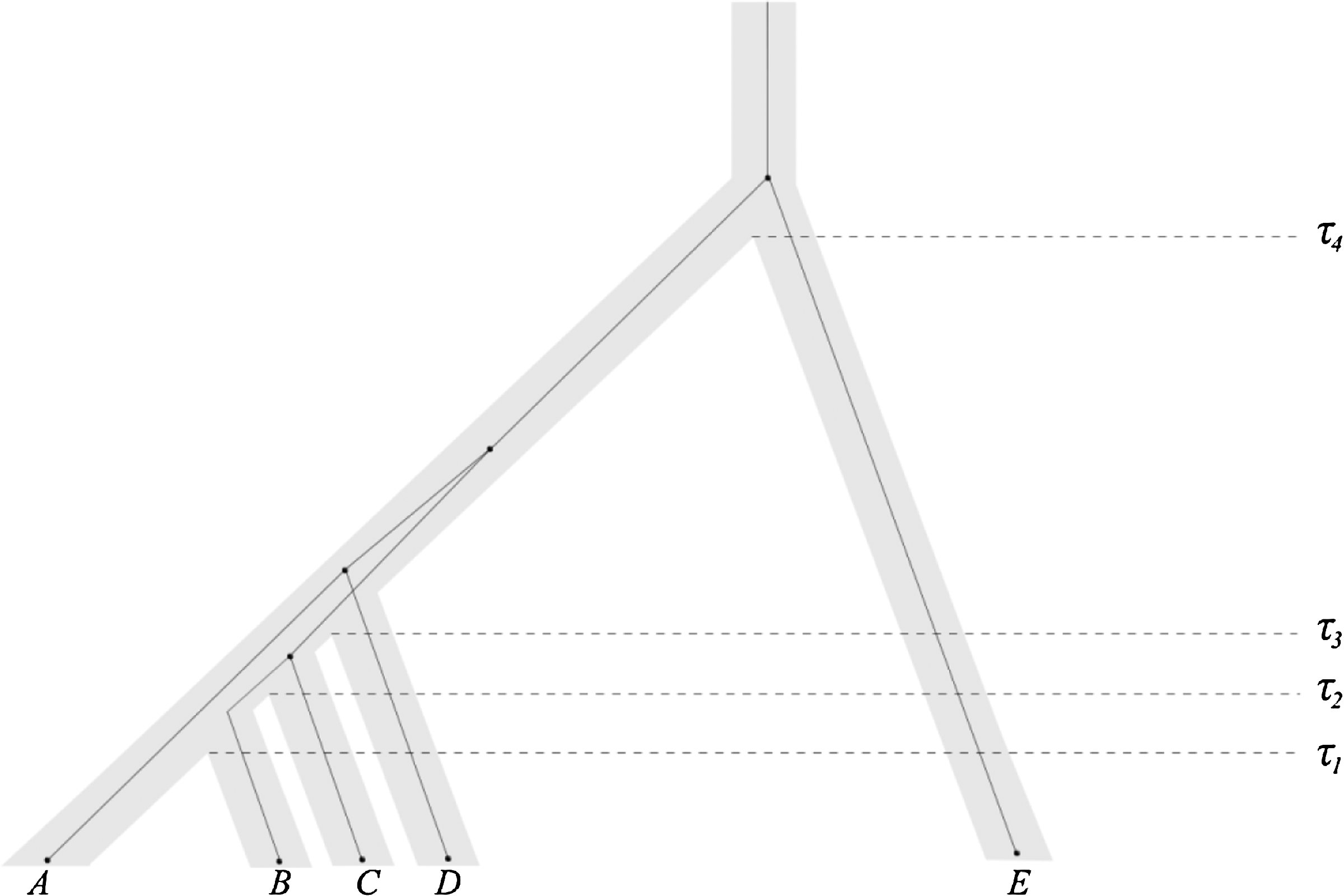
The five-taxon species tree in the anomaly zone used for assessing the accuracy of estimators of pairwise divergence times. The simulation results in Figure 7 rely on this species tree. Divergence times are given by τ1 = 0.025, τ2 = 0.02625, τ3 = 0.0275, and τ4 = 0.5275 coalescent units, and the tree is not drawn to scale. Dark lines show one anomalous gene tree, (((BC)(AD))E). Under the multispecies coalescent model, this gene tree is more likely to occur than the gene tree matching the species tree, ((((AB)C)D)E).
To evaluate the accuracy with which each method reconstructs the topology, we consider the proportion of sampled sets of gene trees that accurately predict the species tree topology. For this analysis, a set of random five-taxon species trees was generated under the Yule model (Kulkarni, 2010). Briefly, for each tree, a split into two branches is taken at the root. Subsequent bifurcations have an equal probability of occurring on each branch, and the waiting time from the (i − 1)st bifurcation to the (i)th bifurcation is exponentially distributed with mean 1/(iλ For our simulations, we take λ = 1. Bifurcations continue until the external branches of a five-taxon tree have evolved, that is, until the time of the fifth bifurcation (the moment when the sixth external branch is formed). Because sampling is not likely to occur exactly at the time of the fifth bifurcation, we truncate the last branches of the species tree, with the time of truncation chosen uniformly between the times of the fourth and fifth bifurcations.
A set of 50,000 true species trees was generated following this procedure. Using the coalescent simulator ms (Hudson, 2002), one set of five gene trees, representing five loci, was then simulated for each of the true species trees, and divergence times for each pair of taxa were estimated with each of the eight methods. The same set of true species trees, and the same set of simulated gene trees for each species tree, were used to evaluate each method. Species tree estimates were constructed using a hierarchical clustering procedure. Single-linkage was defined to be the clustering method of GLASS by Mossel and Roch (2010). In single-linkage clustering, the two taxa with the shortest distance are grouped; distances between clusters are then recalculated, where the distance between two clusters A and B is defined as the shortest distance between one taxon from cluster A and one from cluster B, considering all such possible pairs of taxa. The two clusters with the shortest distance are grouped and the process is repeated until a single cluster remains. Because MAC, like GLASS, evaluates a minimum over loci, single-linkage, with its minimization procedure for computing distances between clusters, was taken to be the appropriate choice for MAC as well. To make results comparable between improved and original methods, single-linkage clustering was also used for iGLASS and iMAC. For SD, iSD, STEAC, and iSTEAC, where the mean is taken over loci, it is natural to use a clustering method that infers each node height by taking the mean over pairs of taxa that find their common ancestor at the node; because UPGMA defines the distance between cluster A and cluster B as the mean node height of all pairs of taxa, one from cluster A and the other from cluster B, UPGMA was used for these methods.
Figure 7 shows the bias and MSE observed for estimates of pairwise divergence times on the simulated data. Both bias and MSE are reduced considerably by the four improved methods, compared with the original analogues that do not incorporate a partial bias correction. The bias and MSE values are also quite similar to those in corresponding cases from Figure 3; that is, the bias and MSE in pairwise divergence time estimates in the larger tree are similar to those that would be predicted if each pair of taxa constituted a separate two-taxon tree.
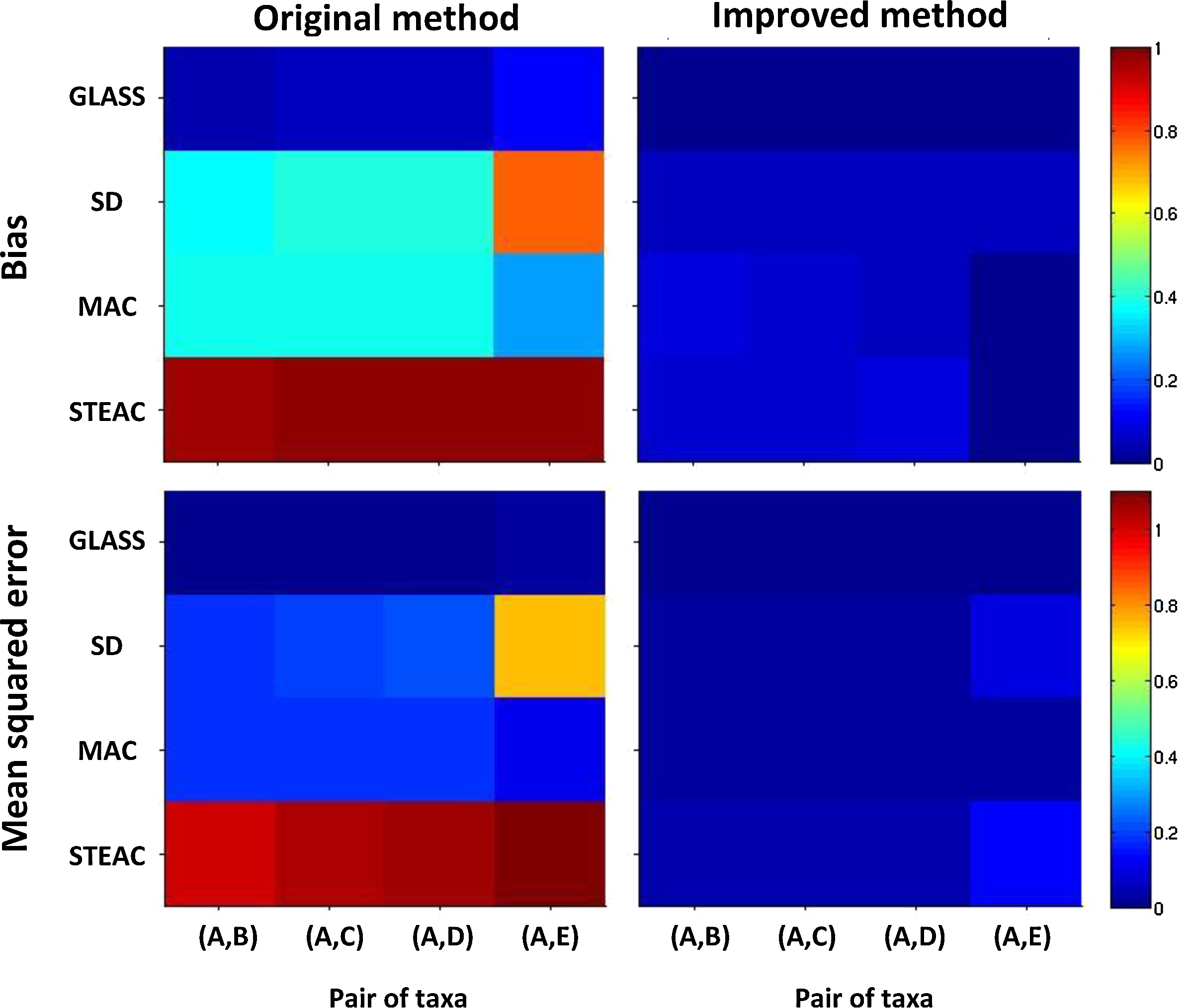
Bias and mean squared error in the estimation of pairwise divergence times for a five-taxon species tree in the anomaly zone. Two lineages were sampled from each taxon at each of five loci. Values were computed using 50,000 replicate sets of five gene trees, generated separately for each method. The species tree from which gene trees were sampled is shown in Figure 6. Results are shown only for (A,B), (A,C), (A,D), and (A,E) because pairs with the same divergence times produce similar results.
Values for our second measure of accuracy, the proportion of species trees reconstructed correctly, appear in Figure 8. Each method is seen to have an increased accuracy as more loci are sampled. The differences in accuracy among the four original methods are substantial. GLASS performs best, with >90% accuracy when ten loci are considered. MAC has >80% percent accuracy at ten loci, compared with ∼70% for SD and STEAC. Each improved method infers the correct tree topology about as often as its corresponding original method, with a slight but noticeable decrease in accuracy for iGLASS compared with GLASS and iMAC compared with MAC, and almost no difference between iSTEAC and STEAC or between iSD and SD.
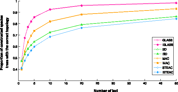
Fraction of species trees reconstructed from gene trees, sampled at a given number of loci, which had the correct species tree topology. The set of species trees considered was a collection of 50,000 randomly sampled five-taxon trees, as described in Section 3.3.
Why do the original and improved methods produce similar accuracy in estimating the tree topology? For each of the methods, g(τ
AB
) is monotonic in τ
AB
(Fig. 5B). For example, if the divergence times between taxa X and Y and between taxa Z and W were estimated to be
4. Discussion
We have shown through simulations that the iGLASS, iSD, iMAC, and iSTEAC estimators of species divergence times have lower biases and mean squared errors than do the original GLASS, SD, MAC, and STEAC estimators, and that these improvements are seen, to varying degrees, under a range of divergence times, numbers of loci, and numbers of lineages sampled. In this section, we place these results in context with respect to the literature, describe limitations of the work, and suggest some problems for future research.
As genetic studies acquire increasingly large amounts of data, computationally fast methods that reconstruct species tree topologies from gene trees while providing accurate branch length estimates are increasingly important. GLASS, SD, MAC, and STEAC provide efficient alternatives to maximum likelihood and Bayesian methods, which can be prohibitively slow on large data sets. Each of these four methods has its own distinct features. GLASS has been shown to be a consistent estimator of tree topology under the coalescent model as the number of loci increases (Mossel and Roch, 2010). SD uses the fact that minimum coalescence times between two species are consistent estimates of species divergence times as the number of sampled lineages increases (Takahata, 1989), and it is less susceptible than GLASS to erroneous inferences resulting from incorrectly inferred gene trees (Liu et al., 2009). In using means at individual loci rather than minima, MAC and STEAC are less susceptible than GLASS and SD to the possibility of divergence time estimates of zero in cases with little genetic variation; STEAC has also been shown to be consistent for the estimation of species tree topologies as the number of loci increases (Liu et al., 2009), and it is easy to compute. Our improved iSD, iMAC, and iSTEAC methods, together with the iGLASS method of Jewett and Rosenberg (2012), provide a class of estimators that can obtain more accurate branch length estimates while preserving properties that make GLASS, SD, MAC, and STEAC appealing.
Asymptotic running times for all of the original and improved methods except iMAC can be obtained by comparison to GLASS and approximate iGLASS, the complexities of which were derived by Mossel and Roch (2010) and by Jewett and Rosenberg (2012), respectively. Because taking a mean at either step in a method (either among pairwise times within a locus, or over loci, or both) instead of a minimum requires the same amount of time, GLASS, SD, MAC, and STEAC all have running time O(n2LS2 + S3) (Mossel and Roch, 2010), where n is the maximum number of lineages sampled from any taxon, L is the number of loci, and S is the number of taxa. iSTEAC also shares this running time, since the method entails calculating the STEAC estimate and subtracting one from each estimated divergence time. Approximate iGLASS has complexity O(n2LQS + LQ3S2), where Q is a tuning parameter affecting the accuracy of the computations (Jewett and Rosenberg, 2012); when the same number of lineages is sampled at each locus from each taxon, it can be shown that approximate iSD has this same precision as well. When loci differ in sample sizes, by noting that Equation C.1 of Jewett and Rosenberg (2012) must be computed L different times, it can be observed that the running time of approximate iSD becomes O(n2LQS + L2Q3S2).
The computation of the iMAC estimator requires sums over all elements of a certain set of unlabeled tree topologies and over all possible values of the numbers of lineages remaining from each taxon at divergence. As the number of lineages increases, iMAC is factorial in nA and factorial in nB; the complexity of the calculations increases so quickly due primarily to the number of tree topologies that must be considered, but also to the increasing complexity of computing the density of the mean pairwise interspecific coalescence time conditional on each topology. We have obtained exact expressions for iMAC for cases in which up to four lineages are sampled per taxon; for large sample sizes, exact computation of the iMAC estimate is not practical, and it will be desirable to develop an approximate iMAC method similar to approximate iGLASS.
Some limitations to the applicability of our results arise from the assumptions we have made. We considered the multispecies coalescent model, in which species divergences each occur at a single point in time, with no subsequent migration or horizontal gene transfer. Further, we have assumed that the effective sizes of all populations in our model are equal, and we have not considered the effects of mutation. Perhaps most importantly, we have assumed that gene trees are known with certainty; when gene trees are inferred, errors in the inference could substantially affect the methods. A particular problem that would be encountered in real data is inferred node heights that are considerably lower than their true values. For instance, if any estimated interspecific coalescence time in the data is zero, GLASS, which takes the minimum over loci of the minimum of pairwise coalescence times, will necessarily give an estimate of zero, as will iGLASS; simulations have suggested that GLASS can have poor performance in practice (Yang and Warnow, 2011). SD, which takes the mean of minimum coalescence times, and MAC, which takes the minimum of mean coalescence times, may also be susceptible to extreme values; underestimates will then be passed on to iSD and iMAC. STEAC, on the other hand, does not employ minimization, taking a mean of mean coalescence times, and it is less likely to be affected by coalescence times of zero. STEAC has performed well for estimating species tree topologies from erroneous gene trees (Liu et al. 2009), and given a gene tree estimator that produces unbiased estimates of coalescence times, STEAC produces an unbiased mean across loci of mean coalescence times, even if gene trees are not inferred correctly. Thus, iSTEAC, which improves upon STEAC, is also expected to perform reasonably well on estimated gene trees.
We note that all of the improved methods—iGLASS, iSD, iMAC, and iSTEAC—share a common drawback. To avoid negative estimates of speciation times, in all of the methods, we set the divergence time estimate to zero when the corresponding estimate from the original method is smaller than its smallest possible expected value, E0[VAB]. While this choice allows us to reduce bias without introducing unreasonable negative estimates, it can be problematic when an estimated divergence time is less than E0[VAB]. For example, because E0[VAB] for iSTEAC is one coalescent unit, regardless of the number of loci or the numbers of lineages sampled, for any observed estimate that is below one, iSTEAC will provide an estimate of zero. This property of the method limits its utility for small divergence times. For iGLASS, iSD, and iMAC, however, this drawback is less problematic, as divergence time estimates of zero are less likely for these methods. Furthermore, for iGLASS, iSD, and iMAC, the probability of obtaining zero estimates decreases as the amount of data increases. For iGLASS and iMAC, in which a minimum is taken over loci, E0[VAB] approaches zero as the number of loci increases, and for iGLASS and iSD, E0[VAB] approaches zero as the number of lineages sampled at each locus in each population increases. To avoid the problem of producing estimates of zero, for all four methods, one solution is to obtain the improved estimate allowing for negative estimates, and then add the absolute value of the most negative estimate to each of the improved estimates. All estimates will then be nonnegative, and fewer estimates of zero will be produced. We expect that this approach will augment bias by an amount comparable to the bias in the most negative estimate, a value that is likely to be small.
Though our simulations have compared these four methods for a variety of values of the model parameters, a comparison of the results obtained with each of the four methods on real data or simulations with mutation would also be informative. Future work that mathematically considers the effects of mutation on these methods could improve their utility for a wider range of practical studies. Finally, an accurate approximation of iMAC would enable use of this method when large amounts of data are available.
Footnotes
Acknowledgments
Support for this work was provided by the NSF (grants DEB-0716904 and DBI-1146722) and by the Burroughs Wellcome Fund.
Disclosure Statement
No competing financial interests exist.