Sample size is a critical component in the design of any high-throughput genetic screening approach. Sample size determination from assumptions or limited data at the planning stages, though standard practice, may at times be unreliable because of the difficulty of a priori modeling of effect sizes and variance. Methods to update the sample size estimate during the course of the study could improve statistical power. In this article, we introduce an approach to estimate the power and update it continuously during the screen. We use this estimate to decide where to sample next to achieve maximum overall statistical power. Finally, in simulations, we demonstrate significant gains in study recall over the naive strategy of equal sample sizes while maintaining the same total number of samples.
1. Introduction
Historically, genetics has assigned biological functions to genes using model organisms, such as yeast, worms, flies and mice, in so-called forward genetic screens. Genomes are randomly mutated and traits of interest measured as a function of the mutation. In this way, the function of the mutated gene in that trait can be inferred. These approaches have been very successful in identifying genes related to all aspects of organism biology, from basic cellular machinery to behavior and lifespan. For example, the function of the antennapedia gene complex, which underpins much of our knowledge of developmental genetics, was established using this method (Lewis et al., 1980). Despite this success, the recent availability of full genome sequences of many organisms, coupled with powerful new technologies to knock out gene function, has led to the development of several high-throughput genetic screening approaches. An example of such an approach is at HHMI's Janelia Farm Research Campus, where the Fly Olympiad project aims to run a high-throughput behavioral screen in fruit flies to determine the role individual neurons or groups of neurons have on various behaviors.
In the Fly Olympiad, fly lines engineered to have controllable activation and inactivation of neurons (targeted by specific genes) are assayed for a variety of behavioral traits (Pfeiffer et al., 2010; Nern et al., 2011). This will allow inference of specific neurons' involvement in specific behaviors. The massive number of lines and behavioral assays together limit the number of samples that can be run for each line if all lines are to be tested.
As a consequence, determination of minimal required sample size is a central concern in this and other high-throughput studies (Zhang and Heyse, 2009). Undersized sampling may not provide statistical significance of the effect, but measuring ever more samples can use more resources than are necessary and be practically infeasible.
When designing high-throughput screens, researchers often estimate the sample size from a limited set of data, for example as obtained in pilot studies, about the effect size and variance of the response being measured. This sample size determination at the planning stages can be difficult and unreliable, and required sample sizes vary for true positives having small, moderate or large effect sizes.
Indeed, using equal sample sizes for groups with possibly different effects is excessive (König et al., 2007; Brass et al., 2008; Ganesan et al., 2008; Crawley, 2008). In such circumstances, it would be desirable to have the ability to update the sample size estimates using the data accumulated during the course of the screen to maintain maximum overall statistical power.
In this article, we introduce an approach to use the expected power estimated continuously during the screen to decide which lines to sample next in order to achieve maximum overall statistical power. Without loss of generality, throughout the rest of the paper we use terminology from genetic screens for behavioral phenotypes, as in the Fly Olympiad and as discussed elsewhere by Crawley (2008), to demonstrate our method. Our method, however, is equally applicable for other types of high-throughput screens, such as screens for the effects of drugs, RNAi, or other bio-active compounds on biological samples, as long as the sampling is sequential.
2. Problem Formulation
In large high-throughput screens, one performs many independent hypothesis tests. For each test, there are four possible outcomes. Either the alternative hypothesis or the null hypothesis could be actually true, and for each of those two possibilities, our test can either reject the null or not. This results in the aptly-named confusion matrix (Table 1), showing the different outcomes of individual tests. This is also known as a two-way contingency table and is a staple of hypothesis testing and classification literature (see http://en.wikipedia.org/wiki/Receiver_operating_characteristic#Basic_concept).
Hypothesis Testing Outcomes Confusion Matrix
Actual value
p
n
Total
p′
True positive
False positive
P′
n′
False negative
True negative
N′
Prediction outcome
Total
P
N
For each tested line, the trait of interest can either be affected (p) or unaffected (n), and for either of those cases, our hypothesis test can either reject the null (p′) or fail to reject it (n′). The event p∩p′ is known as a True Positive, while n ∩ p′ is a False Positive, and so on. Over many tests, P′ is the number of rejections, which is equal to the number of true positives (TP) plus the number of false positives (FP). The other numbers around the table are similarly defined.
These outcomes depend on the hypotheses tested and the random samples drawn for each hypothesis test. Summing these outcomes over all tests when P and N are known allows us to define error rates and accuracy. For example, the precision of a screen is defined as TP/(TP + FP) (also known as positive predictive value, or PPV). It can alternately be defined as the expectation of that quantity. In our case, we would like to maximize the number of true positives while maintaining a fixed α, the level of the test. Fixing α results in a fixed number of true null hypotheses that end up being rejected (known as false positives). In classification terminology, we want to maximize the recall (TP/(TP + FN)) while maintaining the specificity (TN/(FP + TN)) constant. (An alternative approach, to maximize precision while maintaining the number of rejections constant, is related but rather more intractable to analysis, and is not considered here.)
We note that the power of a test and the recall over a set of tests are strongly linked. In particular, for a model parameterized by θ, testing for \documentclass{aastex}\usepackage{amsbsy}\usepackage{amsfonts}\usepackage{amssymb}\usepackage{bm}\usepackage{mathrsfs}\usepackage{pifont}\usepackage{stmaryrd}\usepackage{textcomp}\usepackage{portland, xspace}\usepackage{amsmath, amsxtra}\pagestyle{empty}\DeclareMathSizes {10} {9} {7} {6}
\begin{document}
$$ H_0: \theta \in \Theta_0 $$ \end{document} and \documentclass{aastex}\usepackage{amsbsy}\usepackage{amsfonts}\usepackage{amssymb}\usepackage{bm}\usepackage{mathrsfs}\usepackage{pifont}\usepackage{stmaryrd}\usepackage{textcomp}\usepackage{portland, xspace}\usepackage{amsmath, amsxtra}\pagestyle{empty}\DeclareMathSizes {10} {9} {7} {6}
\begin{document}
$$ H_a: \theta \,\notin\, \Theta_0 $$ \end{document}, we have:
\documentclass{aastex}\usepackage{amsbsy}\usepackage{amsfonts}\usepackage{amssymb}\usepackage{bm}\usepackage{mathrsfs}\usepackage{pifont}\usepackage{stmaryrd}\usepackage{textcomp}\usepackage{portland,xspace}\usepackage{amsmath,amsxtra}\pagestyle{empty}\DeclareMathSizes{10}{9}{7}{6}
\begin{document}
\begin{align*}
{\mathbb E} (TP \mid R) = \sum \limits_{i} {\mathbb I} (\theta_i
\,\notin\, \Theta_0) \beta (\theta_i, m_i) \tag{1}\end{align*}\end{document}
where i indexes all the tests in the screen, and β(θi, mi) is the power function of test i parameterized over the model parameters θi and the number of samples in the ith test, mi. R is a vector such that \documentclass{aastex}\usepackage{amsbsy}\usepackage{amsfonts}\usepackage{amssymb}\usepackage{bm}\usepackage{mathrsfs}\usepackage{pifont}\usepackage{stmaryrd}\usepackage{textcomp}\usepackage{portland, xspace}\usepackage{amsmath, amsxtra}\pagestyle{empty}\DeclareMathSizes {10} {9} {7} {6}
\begin{document}
$$ R_i = {\mathbb I} (\theta_i \,\notin \,\Theta_0) $$ \end{document} for all i. Each test is of a random genetic line that has some probability of affecting the measured trait.
Of course, when dealing with a real screen we don't know the value of \documentclass{aastex}\usepackage{amsbsy}\usepackage{amsfonts}\usepackage{amssymb}\usepackage{bm}\usepackage{mathrsfs}\usepackage{pifont}\usepackage{stmaryrd}\usepackage{textcomp}\usepackage{portland, xspace}\usepackage{amsmath, amsxtra}\pagestyle{empty}\DeclareMathSizes {10} {9} {7} {6}
\begin{document}
$$ {\rm I} (\theta_i \,\notin\, \Theta_0) $$ \end{document}. Therefore, we take the expectation over R:
\documentclass{aastex}\usepackage{amsbsy}\usepackage{amsfonts}\usepackage{amssymb}\usepackage{bm}\usepackage{mathrsfs}\usepackage{pifont}\usepackage{stmaryrd}\usepackage{textcomp}\usepackage{portland,xspace}\usepackage{amsmath,amsxtra}\pagestyle{empty}\DeclareMathSizes{10}{9}{7}{6}
\begin{document}
\begin{align*}
{\mathbb E} (TP) = & {\mathbb E}_{R} [{\mathbb E} (TP \mid R)] \tag{2} \\
= & \sum \limits_{i} p_{0, i}^2 \alpha + (1 - p_{0, i}^2) {\mathbb
E} (\beta_i \mid R_i = 1) \tag{3} \end{align*}\end{document}
where p0,i is the probability that the null hypothesis is true for line i (line i's mutation does not affect the trait of interest), and α is the level of the test. (See the Appendix for a derivation of Equation 3.) p0,i is of course unknown, but we can assume an uninformative prior over the hypotheses to get a decent estimate from the data. For notational convenience, we refer to the event \documentclass{aastex}\usepackage{amsbsy}\usepackage{amsfonts}\usepackage{amssymb}\usepackage{bm}\usepackage{mathrsfs}\usepackage{pifont}\usepackage{stmaryrd}\usepackage{textcomp}\usepackage{portland, xspace}\usepackage{amsmath, amsxtra}\pagestyle{empty}\DeclareMathSizes {10} {9} {7} {6}
\begin{document}
$$ \{\theta_i \in \Theta_0\} $$ \end{document} as Oi. Let X be the observed data. Then:
\documentclass{aastex}\usepackage{amsbsy}\usepackage{amsfonts}\usepackage{amssymb}\usepackage{bm}\usepackage{mathrsfs}\usepackage{pifont}\usepackage{stmaryrd}\usepackage{textcomp}\usepackage{portland,xspace}\usepackage{amsmath,amsxtra}\pagestyle{empty}\DeclareMathSizes{10}{9}{7}{6}
\begin{document}
\begin{align*}
p_{0, i} \widehat{=} & {\mathbb P} (O_i \mid X) \tag{4} \\ = &
\frac{{\mathbb P} (X \mid O_i) {\mathbb P} (O_i)}{{\mathbb P} (X)}
\tag{5} \\ = & \frac {{\mathbb P} (X \mid O_i) {\mathbb P}(O_i)}{{\mathbb P}(X \mid \overline{O}_i){\mathbb P}(\overline{O}_i) + {\mathbb P}
(X \mid O_i) {\mathbb P} (O_i)} \tag{6} \\ = & \frac {{\mathbb P} (X
\mid \overline{O}_i)}{{\mathbb P}(X \mid \overline{O}_i) + {\mathbb
P} (X \mid O_i)} \quad \hbox{as per our uninformative prior , }{\mathbb P} (O_i) = {\mathbb P}(\overline{O_i}) \tag{7} \end{align*}\end{document}
Equation 4 denotes that we are estimating the lhs quantity. Now we replace the probabilities by the likelihoods, and for the alternative hypothesis we take the maximum likelihood given the data:
\documentclass{aastex}\usepackage{amsbsy}\usepackage{amsfonts}\usepackage{amssymb}\usepackage{bm}\usepackage{mathrsfs}\usepackage{pifont}\usepackage{stmaryrd}\usepackage{textcomp}\usepackage{portland,xspace}\usepackage{amsmath,amsxtra}\pagestyle{empty}\DeclareMathSizes{10}{9}{7}{6}
\begin{document}
\begin{align*}
\widehat{p}_{0, i} \approx \frac{\sup \mathscr{L} (X \mid O_i)} {\sup
\mathscr{L} (X \mid O_i) + \sup \mathscr{L} (X \mid \overline{O}_i)}
\tag {8} \end{align*}\end{document}
(We use “sup \documentclass{aastex}\usepackage{amsbsy}\usepackage{amsfonts}\usepackage{amssymb}\usepackage{bm}\usepackage{mathrsfs}\usepackage{pifont}\usepackage{stmaryrd}\usepackage{textcomp}\usepackage{portland, xspace}\usepackage{amsmath, amsxtra}\pagestyle{empty}\DeclareMathSizes {10} {9} {7} {6}
\begin{document}
$$\mathscr{L} $$ \end{document}” as shorthand for “\documentclass{aastex}\usepackage{amsbsy}\usepackage{amsfonts}\usepackage{amssymb}\usepackage{bm}\usepackage{mathrsfs}\usepackage{pifont}\usepackage{stmaryrd}\usepackage{textcomp}\usepackage{portland, xspace}\usepackage{amsmath, amsxtra}\pagestyle{empty}\DeclareMathSizes {10} {9} {7} {6}
\begin{document}
$$ \sup \limits_{\theta_i \in \Theta_0} \mathscr{L} $$ \end{document}” (or \documentclass{aastex}\usepackage{amsbsy}\usepackage{amsfonts}\usepackage{amssymb}\usepackage{bm}\usepackage{mathrsfs}\usepackage{pifont}\usepackage{stmaryrd}\usepackage{textcomp}\usepackage{portland, xspace}\usepackage{amsmath, amsxtra}\pagestyle{empty}\DeclareMathSizes {10} {9} {7} {6}
\begin{document}
$$ \notin $$ \end{document}, as the case may be).
Having found an estimate of p0,i, and α being set by the experimenter, we now need a reasonable estimate of \documentclass{aastex}\usepackage{amsbsy}\usepackage{amsfonts}\usepackage{amssymb}\usepackage{bm}\usepackage{mathrsfs}\usepackage{pifont}\usepackage{stmaryrd}\usepackage{textcomp}\usepackage{portland, xspace}\usepackage{amsmath, amsxtra}\pagestyle{empty}\DeclareMathSizes {10} {9} {7} {6}
\begin{document}
$$ {\mathbb E} (\beta_i \mid R_i = 1) $$ \end{document}. Here, we use \documentclass{aastex}\usepackage{amsbsy}\usepackage{amsfonts}\usepackage{amssymb}\usepackage{bm}\usepackage{mathrsfs}\usepackage{pifont}\usepackage{stmaryrd}\usepackage{textcomp}\usepackage{portland, xspace}\usepackage{amsmath, amsxtra}\pagestyle{empty}\DeclareMathSizes {10} {9} {7} {6}
\begin{document}
$$ \beta(\theta_i^*, m_i) $$ \end{document}, the estimate of the test power at the maximum likelihood estimate of θi given by the data. Then:
\documentclass{aastex}\usepackage{amsbsy}\usepackage{amsfonts}\usepackage{amssymb}\usepackage{bm}\usepackage{mathrsfs}\usepackage{pifont}\usepackage{stmaryrd}\usepackage{textcomp}\usepackage{portland,xspace}\usepackage{amsmath,amsxtra}\pagestyle{empty}\DeclareMathSizes{10}{9}{7}{6}
\begin{document}
\begin{align*}
\widehat{{\mathbb E}(TP)} = \sum \limits_{i} \widehat{p}_{0, i}^2
\alpha + (1 - \widehat{p}_{0, i}^2) \ \beta(\theta_i^*, m_i)
\tag{9}\end{align*}\end{document}
We then want to formulate a sampling strategy that maximizes this quantity, to obtain the maximum number of true positives for a given test level.
\documentclass{aastex}\usepackage{amsbsy}\usepackage{amsfonts}\usepackage{amssymb}\usepackage{bm}\usepackage{mathrsfs}\usepackage{pifont}\usepackage{stmaryrd}\usepackage{textcomp}\usepackage{portland,xspace}\usepackage{amsmath,amsxtra}\pagestyle{empty}\DeclareMathSizes{10}{9}{7}{6}
\begin{document}
\begin{align*}
\beta_{\max} = \max \limits_{\bf{m}: \|\bf{m} \|_1 = M} {\sum
\limits_{i} \widehat{p}_{0, i}^2 \alpha + (1 - \widehat{p}_{0,
i}^2) \ \beta (\theta_i^*, m_i)} \tag{10}\end{align*}\end{document}
where \documentclass{aastex}\usepackage{amsbsy}\usepackage{amsfonts}\usepackage{amssymb}\usepackage{bm}\usepackage{mathrsfs}\usepackage{pifont}\usepackage{stmaryrd}\usepackage{textcomp}\usepackage{portland, xspace}\usepackage{amsmath, amsxtra}\pagestyle{empty}\DeclareMathSizes {10} {9} {7} {6}
\begin{document}
$$ {\bf m} = (m_1, m_2, \ldots , m_n), \| \cdot \|_1 $$ \end{document} denotes the L1 norm, and M is the total number of samples over all n lines. A simple strategy is to optimize the above expression directly at each timestep. We show in Section 3 that this approach is an effective way to increase statistical power while controlling the total number of samples needed.
2.1. A simple example: z-tests using normally distributed variables of unit variance
We now find an expression for \documentclass{aastex}\usepackage{amsbsy}\usepackage{amsfonts}\usepackage{amssymb}\usepackage{bm}\usepackage{mathrsfs}\usepackage{pifont}\usepackage{stmaryrd}\usepackage{textcomp}\usepackage{portland, xspace}\usepackage{amsmath, amsxtra}\pagestyle{empty}\DeclareMathSizes {10} {9} {7} {6}
\begin{document}
$$ \widehat{{\mathbb E} (TP)} $$ \end{document} assuming that the variable observed under the null is a normal random variable with mean 0 and variance 1. The null hypothesis for each test is that the mean μi is 0, with the alternative hypothesis being that μi ≠ 0. This problem formulation is motivated by the structure of many high-throughput screens, in which the number of control samples is very large, enough to accurately estimate the mean and variance of the controls. Then the test samples for each test can be normalized, and a z-test performed. (Under other assumptions of normality, of course.)
In this case, \documentclass{aastex}\usepackage{amsbsy}\usepackage{amsfonts}\usepackage{amssymb}\usepackage{bm}\usepackage{mathrsfs}\usepackage{pifont}\usepackage{stmaryrd}\usepackage{textcomp}\usepackage{portland, xspace}\usepackage{amsmath, amsxtra}\pagestyle{empty}\DeclareMathSizes {10} {9} {7} {6}
\begin{document}
$$ \widehat{p}_{0, i} = \exp(- m_i \bar{x}_i^2) / (\exp(- m_i
\bar{x}_i^2) + 1) $$ \end{document}, while
In the next section, we show the effects of using a sampling strategy, which we call Betamax, that aims directly to maximize this quantity.
3. Results
Suppose we want to screen 2,000 strains for effect on some variable, but each test is expensive and time-consuming. As a result, we can only run about 12,000 tests, or 6 per strain. This scale is very similar to that seen by the Fly Olympiad at Janelia. Samples of equal size will only allow us to detect the most obviously affected lines. In fact, it may be wasteful to use more samples on some of the lines, since their effect might be obvious after just 2 or 3 samples. In these cases, it would be better to devote extra samples to promising but as yet not statistically significant strains.
We propose to sample the line that offers the highest increase in our current estimate of \documentclass{aastex}\usepackage{amsbsy}\usepackage{amsfonts}\usepackage{amssymb}\usepackage{bm}\usepackage{mathrsfs}\usepackage{pifont}\usepackage{stmaryrd}\usepackage{textcomp}\usepackage{portland, xspace}\usepackage{amsmath, amsxtra}\pagestyle{empty}\DeclareMathSizes {10} {9} {7} {6}
\begin{document}
$$ {\mathbb E} (TP) $$ \end{document}. Thus we would be hill-climbing the total statistical power landscape using a steepest-ascent approach. At each step t, we compute the current sample means and \documentclass{aastex}\usepackage{amsbsy}\usepackage{amsfonts}\usepackage{amssymb}\usepackage{bm}\usepackage{mathrsfs}\usepackage{pifont}\usepackage{stmaryrd}\usepackage{textcomp}\usepackage{portland, xspace}\usepackage{amsmath, amsxtra}\pagestyle{empty}\DeclareMathSizes {10} {9} {7} {6}
\begin{document}
$$ {\mathbb E} (TP)_t $$ \end{document}, and \documentclass{aastex}\usepackage{amsbsy}\usepackage{amsfonts}\usepackage{amssymb}\usepackage{bm}\usepackage{mathrsfs}\usepackage{pifont}\usepackage{stmaryrd}\usepackage{textcomp}\usepackage{portland, xspace}\usepackage{amsmath, amsxtra}\pagestyle{empty}\DeclareMathSizes {10} {9} {7} {6}
\begin{document}
$$ \widehat{{\mathbb E} (TP)}_{i, t + 1} $$ \end{document}, the value of \documentclass{aastex}\usepackage{amsbsy}\usepackage{amsfonts}\usepackage{amssymb}\usepackage{bm}\usepackage{mathrsfs}\usepackage{pifont}\usepackage{stmaryrd}\usepackage{textcomp}\usepackage{portland, xspace}\usepackage{amsmath, amsxtra}\pagestyle{empty}\DeclareMathSizes {10} {9} {7} {6}
\begin{document}
$$ {\mathbb E} (TP) $$ \end{document} when mi is increased by 1, for each i. Then we sample the line that shows the highest \documentclass{aastex}\usepackage{amsbsy}\usepackage{amsfonts}\usepackage{amssymb}\usepackage{bm}\usepackage{mathrsfs}\usepackage{pifont}\usepackage{stmaryrd}\usepackage{textcomp}\usepackage{portland, xspace}\usepackage{amsmath, amsxtra}\pagestyle{empty}\DeclareMathSizes {10} {9} {7} {6}
\begin{document}
$$ \widehat{{\mathbb E} (TP)}_{i, t + 1} $$ \end{document}.
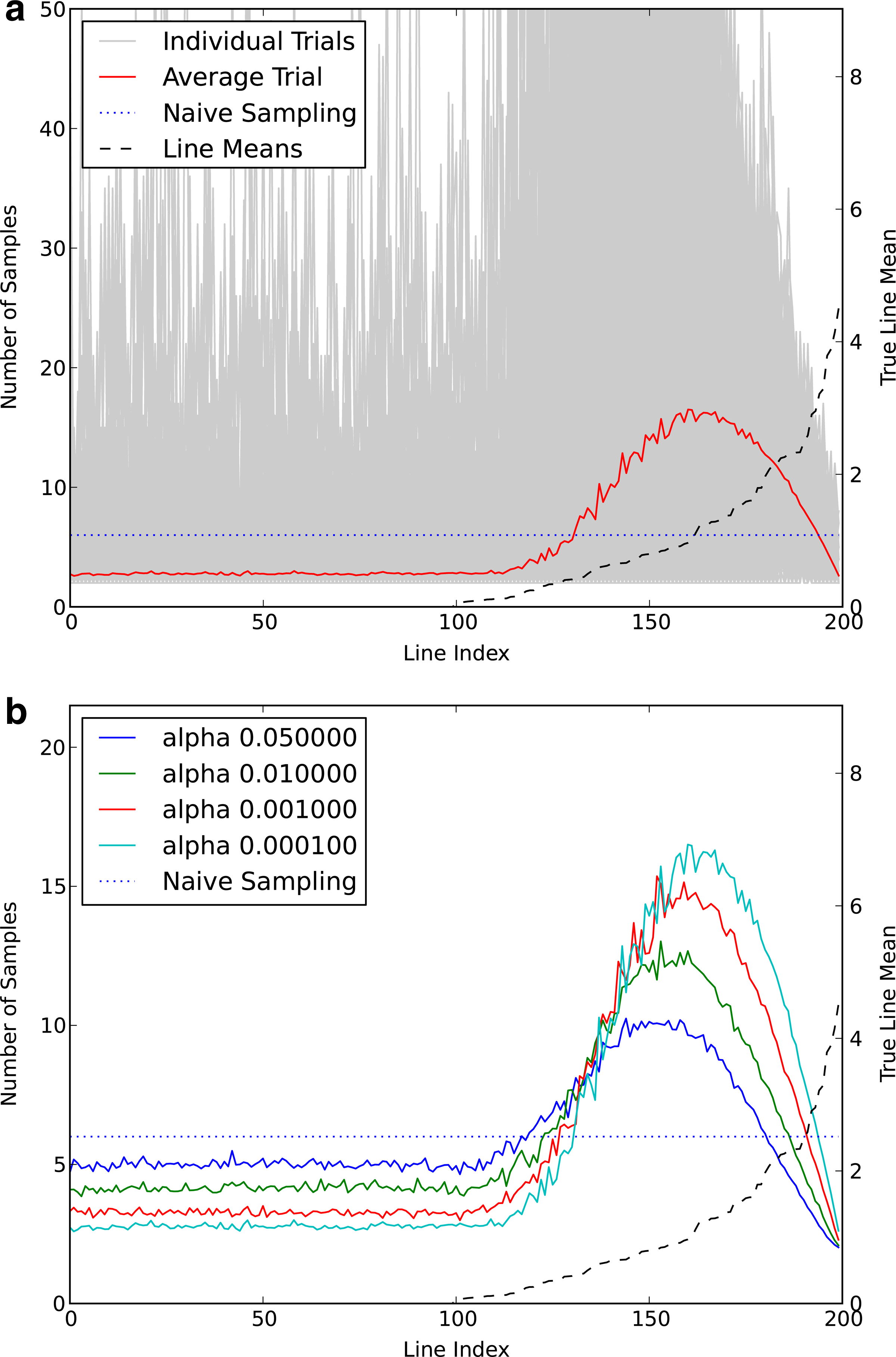
We generated a simulation of 100 null lines and 100 lines having means >0 chosen from an exponential distribution with λ = 1. We began with two samples of each line and a quota of 6 × 200 = 1200 samples. We then sampled according to the line that would maximize our expected power given the current means and m. We show in Figure 1a the resulting number of samples per line for 1,000 simulations, as well as the average across all simulations, for α = 10−4. Our sampling strategy results in fewer samples being used in true null lines or very obvious true positives, with most samples being invested in lines of moderate effect size. By computing the true power (using the actual means, not the sample means) we show that we get on average 50% more true positives than a naive sampling strategy that places an equal number of samples on each line. The smallest and largest improvements observed were 1% and 111%, respectively.
(a) The betamax procedure increases sample size for lines with moderate effect size. The average number of samples for each line from 1,000 simulations is shown in red (sample sizes from individual simulations in gray). The dotted blue line indicates the number of samples when using equal sample sizes for all lines and same total number of samples. True means of each line are shown as the black dashed line—100 null lines and 100 lines with means drawn from Exp(1) (scale on right). (b) Effect of using a different α on average sample size of each line. Note that as α decreases (becomes more stringent), less and less samples are taken from the null and small effect lines, and more are taken from moderate-to-large effect lines.
The effect shown depends on the α chosen, as demonstrated in Figure 1b. For less stringent α, more time is spent sampling null lines since these are more likely to achieve that level of significance early on. As such, the gains are smaller than for very stringent α but still positive on average. For example, for α = 0.01, the average gain is just 5%. However, for high-throughput screens, one usually wants strongly significant lines, since resources for follow-up studies are limited.
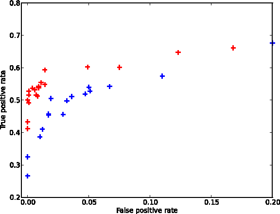
In Figure 2, we present a Receiver Operating Characteristic (ROC) curve comparing the true positive rate (TPR) and false positive rate (FPR) for our optimized sampling procedure Betamax (red) vs equal sample sizes (blue). Note that for low FPR, we obtain up to 30% more true positives than the equal sample size strategy. This demonstrates that the Betamax procedure enables the identification of additional true hits while controlling FPR using the same total number of samples.
ROC values after running Betamax for varying values of α, focused on the low false positive rate, high precision part of the curve. Blue, naive sampling; Red, Betamax sampling.
In Figure 3, we investigate further the shape of the total power \documentclass{aastex}\usepackage{amsbsy}\usepackage{amsfonts}\usepackage{amssymb}\usepackage{bm}\usepackage{mathrsfs}\usepackage{pifont}\usepackage{stmaryrd}\usepackage{textcomp}\usepackage{portland, xspace}\usepackage{amsmath, amsxtra}\pagestyle{empty}\DeclareMathSizes {10} {9} {7} {6}
\begin{document}
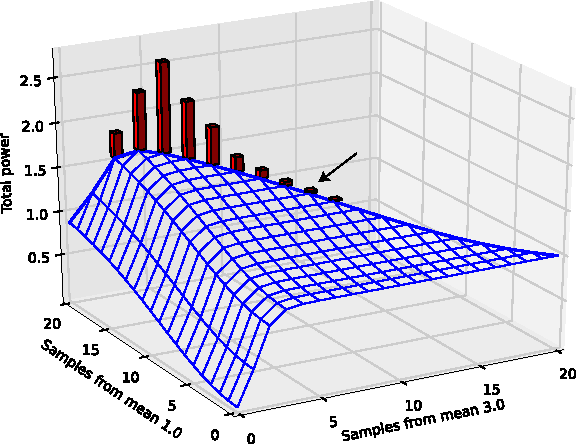
$$ {\mathbb E} (TP) $$ \end{document} as a function of sample sizes for different strains. Note that the total power is essentially flat after just 4 samples of the strain with μ = 3.0. This means that additional samples of this strain provide almost no information for the purposes of the screen. The horizon line (shown in thick blue) represents the total power for a total sample size of 20. The bars indicate the relative frequency with which Betamax arrives at that combination of sample sizes over 1,000 simulations. Although the procedure is stochastic, the vast majority of simulations obtain an improvement in total power over equal sample sizes (indicated by the arrow).
Total power for varying sample sizes with two non-null strains having means 1.0 and 3.0 with level α = 0.001. Histogram indicates relative frequency of Betamax procedure arriving at the corresponding sample sizes. Arrow shows power for equal sample sizes (1.45). The maximum total power, βmax, is 1.88, at (17,3).
Taken together, these simulation results demonstrate the advantage of dynamically adjusting sample sizes, in particular through the Betamax procedure, over simply choosing a fixed sample size for all lines. This suggests significant gains in efficiency to be made in high-throughput screens.
4. Discussion
In this article, we introduced an approach, Betamax, that uses the conditional power calculated continuously during the screen to decide which line to sample next to achieve maximum overall power for a given total number of samples. We have focused on the idea of genetic screens, in which mutant lines are tested for specific traits or behaviors. However, the procedure can be used in any sequential high-throughput screening setting.
For example, sample size adjustment is gaining popularity in pharmaceutical industry drug trials as a technique to save time, resources and money. Different approaches have been proposed in the clinical trial literature. For example, Shih (1992) and Whitehead et al. (2001) propose mid-trial sample size correction, using provisional information collected during the trial. Proschan and Hunsberger (1995), Fisher (1998), Cui et al. (1999), and Jennison and Turnbull (2003) propose a two-stage adaptive design that maintains the Type-I error rate. Extensions to the two-stage adaptive design methods were provided by Liu and Chi (2001), whose method comprises a main stage and an extension stage, where the main stage had sufficient power to reject the null under the expected effect size and the extension stage allowed for increased sample size if the true effect size was smaller than expected. Li et al. (2002) modified the procedure of Proschan and Hunsberger (1995) by relaxing the form of the linear conditional type-I error function, so that adjustments to the final stage critical value did not depend on the outcome of the first stage.
Our approach somewhat generalizes those shown above, by continuously adjusting our sampling strategy, rather than doing it at two specific stages. Of course, this can only be applied when the sampling is sequential in nature. In some cases, including the Fly Olympiad here at Janelia, sampling is sequential but requires the selection of a number of lines in advance, not just the next line. Betamax can be easily modified to accommodate such batch sampling, although we expect performance to somewhat degrade with increasing batch size.
One potential drawback of our approach is that the α level needs to be set in advance. (The ROC curves in Figure 2 are disjointed because each point is the result of a separate stochastic simulation set at a specific α, rather than varying α at the end of one run.) However, even though we explicitly optimized true positives, a side effect of our procedure is to push false positives below the level of significance, which means the false positive rate decreases as the true positive rate increases. This means that the observed level will always be smaller than the α set in advance, which should be acceptable for most applications.
Another potential pitfall is our simple optimization method. As can be seen in Figure 3, the conditional power function β is non-convex over the sample size m. In order to maximize β, we use a greedy hill climbing technique (Russell and Norvig, 2003) that is good for finding the local optimum but is not guaranteed to find the global optimum. The relative simplicity makes it a popular first choice amongst optimization techniques, but more advanced algorithms such as simulated annealing (Kirkpatrick et al., 1983) may give better results.
Further, in order to maximize β, we are essentially taking a multi-dimensional derivative and choosing the dimension with the steepest gradient to decide where to sample next (Fig. 3). Estimating derivatives, however, is highly sensitive to noise in the data. Therefore, methods to estimate derivatives that are more robust to noise would improve our estimates of E(TP)i,t+1, and thus improve performance of the procedure.
Further improvements may be found in our estimate of the total power given the data. We estimate β using the method of moments, substituting for the population mean the sample mean, which is very noisy, since we start with a very low sample size. Other methods of parameter estimation, such as maximum-likelihood estimation, might provide better estimates and therefore improve performance of our method.
The source code for Betamax is freely available under an MIT license (at https://github.com/jni/betamax). We have only provided the simple example of Gaussian simulation, but the particulars of equation 10 are general to any distribution. We leave this for future work.
5. Appendix
A. Derivation of expected number of true positives
And we estimate E(β|μ ≠ 0,X) as the power function of the Z-test at \documentclass{aastex}\usepackage{amsbsy}\usepackage{amsfonts}\usepackage{amssymb}\usepackage{bm}\usepackage{mathrsfs}\usepackage{pifont}\usepackage{stmaryrd}\usepackage{textcomp}\usepackage{portland, xspace}\usepackage{amsmath, amsxtra}\pagestyle{empty}\DeclareMathSizes {10} {9} {7} {6}
\begin{document}
$$ \mu = {\bar X} $$ \end{document}, the MLE of μ. This is the present p-value of the test, but when looking ahead it becomes the p-value if we had more samples with the same mean.
C. Derivation of the power function for a normal distribution
Derivation of power function of test i parameterized over mean μi and number of samples in the ith test mi under assumptions of normality.
\documentclass{aastex}\usepackage{amsbsy}\usepackage{amsfonts}\usepackage{amssymb}\usepackage{bm}\usepackage{mathrsfs}\usepackage{pifont}\usepackage{stmaryrd}\usepackage{textcomp}\usepackage{portland,xspace}\usepackage{amsmath,amsxtra}\pagestyle{empty}\DeclareMathSizes{10}{9}{7}{6}
\begin{document}
\begin{align*}
\beta (\mu_i, m_i) = & {\mathbb P}(\overline{Y} >
\frac{Z_{\alpha}}{\sqrt{m_i}}) + {\mathbb P} (\overline{Y} < - \frac{Z_{\alpha}}{\sqrt{m_i}}) \\ = & {\mathbb P} (\overline{Y} - \mu_i > \frac{Z_{\alpha}}{\sqrt{m_i}} - \mu_i) + {\mathbb P} (\overline{Y} - \mu_i < - \frac{Z_{\alpha}} {\sqrt{m_i}} - \mu_i)\\ = & {\mathbb P} (\sqrt{m_i} (\overline{Y} - \mu_i) > Z_{\alpha} - \sqrt{m_i} \mu_i) + {\mathbb P} (\sqrt{m_i} (\overline{Y} - \mu_i) < - Z_{\alpha} - \sqrt{m_i} \mu_i) \\ = & 1 - \Phi (Z_{\alpha} - \sqrt{m_i} \mu_i) + \Phi (- Z_{\alpha} - \sqrt{m_i} \mu_i) \\ = & \Phi (\sqrt{m_i} \mu_i - Z_{\alpha}) + \Phi (- Z_{\alpha} - \sqrt{m_i} \mu_i)
\end{align*}\end{document}
Footnotes
Acknowledgments
We thank Dr. Simon Tavaré for comments on an earlier draft of the article.
Disclosure Statement
No competing financial interests exist.
References
1.
BrassA.L., DykxhoornD.M., BenitaY.et al.2008. Identification of host proteins required for HIV infection through a functional genomic screen. Science, 319:921–926.
2.
CrawleyJ.N.2008. Behavioral phenotyping strategies for mutant mice. Neuron, 57:809–818.
3.
CuiL., HungH.M., WangS. J.1999. Modification of sample size in group sequential clinical trials. Biometrics, 55:853–857.
GanesanA. K., HoH., BodemannB.et al.2008. Genome-wide siRNA-based functional genomics of pigmentation identifies novel genes and pathways that impact melanogenesis in human cells. PLoS Genet., 4:e1000298.
6.
JennisonC., TurnbullB. W.2003. Mid-course sample size modification in clinical trials based on the observed treatment effect. Stat. Med., 22:971–993.
7.
KirkpatrickS., GelattC. D., VecchiM. P.1983. Optimization by simulated annealing. Science, 220:671–680.
8.
KönigR., ChiangC.-Y., TuB. P.et al.2007. A probability-based approach for the analysis of large-scale RNAi screens. Nat. Methods, 4:847–849.
9.
LewisR. A., KaufmanT. C., DenellR. E.et al.1980. Genetic analysis of the Antennapedia gene complex (Ant-C) and adjacent chromosomal regions of Drosophila Melanogaster. I. Polytene chromosome segments 84b-D. Genetics, 95:367–381.
10.
LiG., ShihW. J., XieT.et al.2002. A sample size adjustment procedure for clinical trials based on conditional power. Biostatistics, 3:277–287.
11.
LiuQ., ChiG. Y.2001. On sample size and inference for two-stage adaptive designs. Biometrics, 57:172–177.
12.
NernA., PfeifferB. D., SvobodaK.et al.2011. Multiple new site-specific recombinases for use in manipulating animal genomes. Proc. Natl. Acad. Sci. U.S.A., 108:14198–14203.
13.
PfeifferB. D., NgoT. T., HibbardK. L.et al.2010. Refinement of tools for targeted gene expression in Drosophila. Genetics, 186:735–755.
14.
ProschanM. A., HunsbergerS. A.1995. Designed extension of studies based on conditional power. Biometrics, 51:1315–1324.
15.
RussellS. J., NorvigP.2003. Artificial Intelligence: A Modern Approach. Pearson Education: Saddle River, NJ.
16.
ShihW. J.1992. Sample size re-estimation in clinical trials, 285–301. PeaceK.Biopharmaceutical Sequential Statistical Applications. Dekker: New York.