Dirichlet mixtures provide an elegant formalism for constructing and evaluating protein multiple sequence alignments. Their use requires the inference of Dirichlet mixture priors from curated sets of accurately aligned sequences. This article addresses two questions relevant to such inference: of how many components should a Dirichlet mixture consist, and how may a maximum-likelihood mixture be derived from a given data set. To apply the Minimum Description Length principle to the first question, we extend an analytic formula for the complexity of a Dirichlet model to Dirichlet mixtures by informal argument. We apply a Gibbs-sampling based approach to the second question. Using artificial data generated by a Dirichlet mixture, we demonstrate that our methods are able to approximate well the true theory, when it exists. We apply our methods as well to real data, and infer Dirichlet mixtures that describe the data better than does a mixture derived using previous approaches.
1. Introduction
Multiple protein sequence alignment is a central problem in computational molecular biology. A powerful and elegant formalism underpinning one approach to multiple sequence alignment is that of Dirichlet mixtures (Brown et al., 1993; Sjölander et al., 1996; Altschul et al., 2010). Intuitively, it is assumed that positions within a protein can be thought of as falling into a small number of classes. Each such class may be described by its frequency within proteins, by a set of typical amino acid probabilities for protein positions belonging to the class, and by how far the probabilities associated with a specific position tend to diverge from these typical values. A Dirichlet mixture (DM) captures these notions formally.
There is no plausible way to construct from first principles a DM appropriate for protein sequence comparison, and DMs for this purpose are therefore derived from curated sets of protein multiple alignments, generally by seeking a maximum-likelihood DM (Brown et al., 1993; Sjölander et al., 1996). An immediate problem that arises is how many classes or components such a DM should have, but no systematic guidance for answering his question has been published. As is generally the case in model selection, the more components and therefore parameters a DM is allowed to have, the better it will be able to describe a given set of data, but a DM with too many components will tend to overfit the data. The Minimum Description Length (MDL) principle (Grünwald, 2007) provides a way to deal with this problem. It implies that one should seek to minimize the description length of the data given the maximum-likelihood M-component DM, plus a measure of the complexity of the set of all M-component DMs. To apply the principle, we require both a method for finding maximum-likelihood DMs, and a formula for the complexity of a Dirichlet mixture model.
This article is organized as follows. First, we review the essentials of multinomial, Dirichlet, and Dirichlet mixture distributions, and of MDL theory. Second, we present heuristic arguments for extending to Dirichlet mixtures an analytic formula for the complexity of a single Dirichlet distribution model. Third, we present a Gibbs-sampling algorithm for seeking a maximum-likelihood DM to describe a given set of multiple alignment data. Other algorithmic approaches to this problem have been developed previously (Brown et al., 1993; Sjölander et al., 1996). Fourth, we apply our complexity formula and optimization algorithm to artificial data generated by a known DM, to study whether our method allows us to recover the DM's number of components, and to estimate its parameters accurately. Finally, we apply our method to real data from protein multiple alignments, and compare our results to earlier ones.
2. Review
2.1. Multinomial and Dirichlet distributions, and Dirichlet mixtures
Statistical approaches to protein sequence comparison analyze the probabilities \documentclass{aastex}\usepackage{amsbsy}\usepackage{amsfonts}\usepackage{amssymb}\usepackage{bm}\usepackage{mathrsfs}\usepackage{pifont}\usepackage{stmaryrd}\usepackage{textcomp}\usepackage{portland, xspace}\usepackage{amsmath, amsxtra}\pagestyle{empty}\DeclareMathSizes {10} {9} {7} {6}\begin{document}$$\boldsymbol{\vec p}$$\end{document} for the various amino acids to appear at particular protein positions. Baysian approaches require the specification of prior probabilities over the space of all possible \documentclass{aastex}\usepackage{amsbsy}\usepackage{amsfonts}\usepackage{amssymb}\usepackage{bm}\usepackage{mathrsfs}\usepackage{pifont}\usepackage{stmaryrd}\usepackage{textcomp}\usepackage{portland, xspace}\usepackage{amsmath, amsxtra}\pagestyle{empty}\DeclareMathSizes {10} {9} {7} {6}\begin{document}$$\boldsymbol{\vec p}$$\end{document}, and for mathematical convenience these priors are almost always taken to be Dirichlet distributions or Dirichlet mixtures. In this section, we review briefly the relevant mathematical concepts.
A multinomial distribution over an alphabet of L letters is described by an L-component vector of positive probabilities \documentclass{aastex}\usepackage{amsbsy}\usepackage{amsfonts}\usepackage{amssymb}\usepackage{bm}\usepackage{mathrsfs}\usepackage{pifont}\usepackage{stmaryrd}\usepackage{textcomp}\usepackage{portland, xspace}\usepackage{amsmath, amsxtra}\pagestyle{empty}\DeclareMathSizes {10} {9} {7} {6}\begin{document}$$\boldsymbol{\vec p}$$\end{document}, with \documentclass{aastex}\usepackage{amsbsy}\usepackage{amsfonts}\usepackage{amssymb}\usepackage{bm}\usepackage{mathrsfs}\usepackage{pifont}\usepackage{stmaryrd}\usepackage{textcomp}\usepackage{portland, xspace}\usepackage{amsmath, amsxtra}\pagestyle{empty}\DeclareMathSizes {10} {9} {7} {6}\begin{document}$$\sum\nolimits_{j = 1}^L p_j = 1$$\end{document}. Because of the constraint, the space Ω of all possible multinomials is L − 1 dimensional. One may imagine the probabilities for the various amino acids appearing at a particular protein position as described by a particular multinomial.
Bayesian statistics require the specification of a prior probability density over the multinomial space Ω. Such a prior should capture as well as possible one's general knowledge concerning proteins. For example, multinomials may be favored, among others, in which all and only the hydrophobic residues have high probabilities, whereas multinomials may be disfavored in which both hydrophobic and charged residues have high probabilities. Although a prior distribution θ may take any form one wishes, for analytic and computational convenience it is best to require that θ be a Dirichlet distribution or a Dirichlet mixture.
A Dirichlet distribution is a probability density over Ω. A particular Dirichlet distribution may be specified by an L-dimensional parameter vector \documentclass{aastex}\usepackage{amsbsy}\usepackage{amsfonts}\usepackage{amssymb}\usepackage{bm}\usepackage{mathrsfs}\usepackage{pifont}\usepackage{stmaryrd}\usepackage{textcomp}\usepackage{portland, xspace}\usepackage{amsmath, amsxtra}\pagestyle{empty}\DeclareMathSizes {10} {9} {7} {6}\begin{document}$$\boldsymbol{\vec \alpha}$$\end{document}, with all αj positive, and it is convenient to define \documentclass{aastex}\usepackage{amsbsy}\usepackage{amsfonts}\usepackage{amssymb}\usepackage{bm}\usepackage{mathrsfs}\usepackage{pifont}\usepackage{stmaryrd}\usepackage{textcomp}\usepackage{portland, xspace}\usepackage{amsmath, amsxtra}\pagestyle{empty}\DeclareMathSizes {10} {9} {7} {6}\begin{document}$$\alpha^* \equiv \sum\nolimits_{j = 1}^L \alpha_j$$\end{document}. The density of this distribution at \documentclass{aastex}\usepackage{amsbsy}\usepackage{amsfonts}\usepackage{amssymb}\usepackage{bm}\usepackage{mathrsfs}\usepackage{pifont}\usepackage{stmaryrd}\usepackage{textcomp}\usepackage{portland, xspace}\usepackage{amsmath, amsxtra}\pagestyle{empty}\DeclareMathSizes {10} {9} {7} {6}\begin{document}$$\boldsymbol{\vec x}$$\end{document} is defined as
\documentclass{aastex}\usepackage{amsbsy}\usepackage{amsfonts}\usepackage{amssymb}\usepackage{bm}\usepackage{mathrsfs}\usepackage{pifont}\usepackage{stmaryrd}\usepackage{textcomp}\usepackage{portland, xspace}\usepackage{amsmath, amsxtra}\pagestyle{empty}\DeclareMathSizes {10} {9} {7} {6}\begin{document}\begin{align*}
f (\boldsymbol{\vec x}) = Z \prod_{j = 1}^L x_j^{\alpha_j - 1}, \tag{1}
\end{align*}\end{document}
where the normalizing scalar \documentclass{aastex}\usepackage{amsbsy}\usepackage{amsfonts}\usepackage{amssymb}\usepackage{bm}\usepackage{mathrsfs}\usepackage{pifont}\usepackage{stmaryrd}\usepackage{textcomp}\usepackage{portland, xspace}\usepackage{amsmath, amsxtra}\pagestyle{empty}\DeclareMathSizes {10} {9} {7} {6}\begin{document}$$Z = \Gamma (\alpha^*) / \prod\nolimits_{j = 1}^L \Gamma (\alpha_j)$$\end{document} ensures that integrating f over its domain Ω yields 1. The special case of all αj = 1 corresponds to the uniform density.
One may show that the expected value of \documentclass{aastex}\usepackage{amsbsy}\usepackage{amsfonts}\usepackage{amssymb}\usepackage{bm}\usepackage{mathrsfs}\usepackage{pifont}\usepackage{stmaryrd}\usepackage{textcomp}\usepackage{portland, xspace}\usepackage{amsmath, amsxtra}\pagestyle{empty}\DeclareMathSizes {10} {9} {7} {6}\begin{document}$$\boldsymbol{\vec x}$$\end{document} is \documentclass{aastex}\usepackage{amsbsy}\usepackage{amsfonts}\usepackage{amssymb}\usepackage{bm}\usepackage{mathrsfs}\usepackage{pifont}\usepackage{stmaryrd}\usepackage{textcomp}\usepackage{portland, xspace}\usepackage{amsmath, amsxtra}\pagestyle{empty}\DeclareMathSizes {10} {9} {7} {6}\begin{document}$$\boldsymbol{\vec q} = \boldsymbol{\vec \alpha} / \alpha^*$$\end{document}, and it is sometimes convenient to specify a Dirichlet distribution using the alternative parametrization (\documentclass{aastex}\usepackage{amsbsy}\usepackage{amsfonts}\usepackage{amssymb}\usepackage{bm}\usepackage{mathrsfs}\usepackage{pifont}\usepackage{stmaryrd}\usepackage{textcomp}\usepackage{portland, xspace}\usepackage{amsmath, amsxtra}\pagestyle{empty}\DeclareMathSizes {10} {9} {7} {6}\begin{document}$$\boldsymbol{\vec q}$$\end{document}, α*). Because only L − 1 of the components of \documentclass{aastex}\usepackage{amsbsy}\usepackage{amsfonts}\usepackage{amssymb}\usepackage{bm}\usepackage{mathrsfs}\usepackage{pifont}\usepackage{stmaryrd}\usepackage{textcomp}\usepackage{portland, xspace}\usepackage{amsmath, amsxtra}\pagestyle{empty}\DeclareMathSizes {10} {9} {7} {6}\begin{document}$$\boldsymbol{\vec q}$$\end{document} are independent, there are still L free parameters. The “location parameters” \documentclass{aastex}\usepackage{amsbsy}\usepackage{amsfonts}\usepackage{amssymb}\usepackage{bm}\usepackage{mathrsfs}\usepackage{pifont}\usepackage{stmaryrd}\usepackage{textcomp}\usepackage{portland, xspace}\usepackage{amsmath, amsxtra}\pagestyle{empty}\DeclareMathSizes {10} {9} {7} {6}\begin{document}$$\boldsymbol{\vec q}$$\end{document} specify the center of mass of the distribution, while the “concentration parameter” α* specifies how tightly the probability density is concentrated near \documentclass{aastex}\usepackage{amsbsy}\usepackage{amsfonts}\usepackage{amssymb}\usepackage{bm}\usepackage{mathrsfs}\usepackage{pifont}\usepackage{stmaryrd}\usepackage{textcomp}\usepackage{portland, xspace}\usepackage{amsmath, amsxtra}\pagestyle{empty}\DeclareMathSizes {10} {9} {7} {6}\begin{document}$$\boldsymbol{\vec q}$$\end{document}. Large values of α* correspond to densities very concentrated near \documentclass{aastex}\usepackage{amsbsy}\usepackage{amsfonts}\usepackage{amssymb}\usepackage{bm}\usepackage{mathrsfs}\usepackage{pifont}\usepackage{stmaryrd}\usepackage{textcomp}\usepackage{portland, xspace}\usepackage{amsmath, amsxtra}\pagestyle{empty}\DeclareMathSizes {10} {9} {7} {6}\begin{document}$$\boldsymbol{\vec q}$$\end{document}, whereas values of α* near 0 correspond to densities concentrated near the boundaries of Ω.
Different protein positions are under different physical constraints and selective pressures, but it may be imagined that most positions fall into one of several broad categories, each with its own amino acid preferences. This implies that multiple distinct regions of multinomial space should have high prior probabilities. A single Dirichlet distribution in general cannot model such a density, but a Dirichlet mixture (DM) can. A DM is a probability density over Ω that is a simple linear combination of a finite number M of Dirichlet distributions, each called a Dirichlet component. Formally, it is defined by M Dirichlet distributions with respective parameters \documentclass{aastex}\usepackage{amsbsy}\usepackage{amsfonts}\usepackage{amssymb}\usepackage{bm}\usepackage{mathrsfs}\usepackage{pifont}\usepackage{stmaryrd}\usepackage{textcomp}\usepackage{portland, xspace}\usepackage{amsmath, amsxtra}\pagestyle{empty}\DeclareMathSizes {10} {9} {7} {6}\begin{document}$$\boldsymbol{\vec \alpha}_i$$\end{document}, and a set of M positive “mixture parameters” \documentclass{aastex}\usepackage{amsbsy}\usepackage{amsfonts}\usepackage{amssymb}\usepackage{bm}\usepackage{mathrsfs}\usepackage{pifont}\usepackage{stmaryrd}\usepackage{textcomp}\usepackage{portland, xspace}\usepackage{amsmath, amsxtra}\pagestyle{empty}\DeclareMathSizes {10} {9} {7} {6}\begin{document}$$\boldsymbol{\vec m}$$\end{document} that sum to 1. Because of this last constraint, a DM has ML + M − 1 free parameters. Defining \documentclass{aastex}\usepackage{amsbsy}\usepackage{amsfonts}\usepackage{amssymb}\usepackage{bm}\usepackage{mathrsfs}\usepackage{pifont}\usepackage{stmaryrd}\usepackage{textcomp}\usepackage{portland, xspace}\usepackage{amsmath, amsxtra}\pagestyle{empty}\DeclareMathSizes {10} {9} {7} {6}\begin{document}$$\alpha^*_i \equiv \sum\nolimits_{j = 1}^L \alpha_{i, j}$$\end{document}, the center of mass of a DM is simply \documentclass{aastex}\usepackage{amsbsy}\usepackage{amsfonts}\usepackage{amssymb}\usepackage{bm}\usepackage{mathrsfs}\usepackage{pifont}\usepackage{stmaryrd}\usepackage{textcomp}\usepackage{portland, xspace}\usepackage{amsmath, amsxtra}\pagestyle{empty}\DeclareMathSizes {10} {9} {7} {6}\begin{document}$$\sum\nolimits_ {i = 1} ^M m_i \frac \boldsymbol{\vec \alpha}_i {\alpha^*_i} = \sum\nolimits_ {i = 1} ^M m_i \boldsymbol{\vec q}_i$$\end{document}.
For Bayesian analysis, the signal advantage of using a Dirichlet prior θ over Ω is that after the observation of a single letter a, the posterior is also a Dirichlet distribution θ′, with parameters identical to θ, except that \documentclass{aastex}\usepackage{amsbsy}\usepackage{amsfonts}\usepackage{amssymb}\usepackage{bm}\usepackage{mathrsfs}\usepackage{pifont}\usepackage{stmaryrd}\usepackage{textcomp}\usepackage{portland, xspace}\usepackage{amsmath, amsxtra}\pagestyle{empty}\DeclareMathSizes {10} {9} {7} {6}\begin{document}$$\alpha^{\prime}_a = \alpha_a + 1$$\end{document}. Similarly, if the prior is a DM, the posterior is also a DM, with parameters that are easy to calculate (Brown et al., 1993; Sjölander et al., 1996; Altschul et al., 2010). The class of DMs is rich enough to model well a broad range of prior beliefs.
2.2. Issues in inferring Dirichlet mixture priors
Because there is no plausible way to infer a DM appropriate for protein sequence comparison from theory alone, DMs for this purpose are derived from curated sets of protein multiple alignments. Intuitively, by examining a “gold standard” set of multiple alignment data, constructed using structural or other considerations, one may develop general knowledge about which multinomials tend best to describe protein alignment columns. Formally, after selecting the number M of components comprising the DM, one seeks the maximum-likelihood DM, i.e., that which assigns the multiple alignment data the greatest probability (Brown et al., 1993; Sjölander et al., 1996). Neither step of this procedure is trivial, and the two may be seen as interrelated. This article studies ways in which each of these two steps may be accomplished.
In general, given a variety of related models with which to describe a set of data, the model with the greatest number of parameters will fit the data best. Too many parameters, however, can result in overfitting—modeling the noise within the data rather than the regularities—which can lead to poor predictions on new data. To avoid this problem, a useful criterion for model selection is the MDL principle. Below, we will describe in detail how the MDL principle may be applied to selecting the number of Dirichlet components.
Given a specific number M of components, the question of how to find a maximum-likelihood DM remains. Taking the likelihood of the data as an objective function, the central problem is that the space of M-component DMs has many local maxima. This classic optimization problem has no known rigorous solution, but there are a variety of fruitful heuristic approaches. Among these is Gibbs sampling, whose application to DM optimization we describe below.
2.3. The minimum description length principle
The MDL principle (Grünwald, 2007) addresses the question of which among several models to choose for describing a set of data. It proposes that the model is best which minimizes the description length of the data given the model, plus the description length of the model. Formalizing these concepts is not trivial (Grünwald, 2007), and for brevity we will confine our review of the MDL approach to those elements relevant to the problem at hand.
We take a theory θ to specify a probability distribution Pθ over the space of all possible sets of data. The description length (in bits) of a set of data D given θ is then defined as DL(D|θ) = −log2[Pθ(D)]. (Throughout this article, we assume logs to be base 2; when natural logarithms are needed, we use the notation ln.) A model \documentclass{aastex}\usepackage{amsbsy}\usepackage{amsfonts}\usepackage{amssymb}\usepackage{bm}\usepackage{mathrsfs}\usepackage{pifont}\usepackage{stmaryrd}\usepackage{textcomp}\usepackage{portland, xspace}\usepackage{amsmath, amsxtra}\pagestyle{empty}\DeclareMathSizes {10} {9} {7} {6}\begin{document}$$\mathfrak {M}$$\end{document} is a parametrized set of theories, and the description length of D given \documentclass{aastex}\usepackage{amsbsy}\usepackage{amsfonts}\usepackage{amssymb}\usepackage{bm}\usepackage{mathrsfs}\usepackage{pifont}\usepackage{stmaryrd}\usepackage{textcomp}\usepackage{portland, xspace}\usepackage{amsmath, amsxtra}\pagestyle{empty}\DeclareMathSizes {10} {9} {7} {6}\begin{document}$$\mathfrak {M}$$\end{document} is defined as \documentclass{aastex}\usepackage{amsbsy}\usepackage{amsfonts}\usepackage{amssymb}\usepackage{bm}\usepackage{mathrsfs}\usepackage{pifont}\usepackage{stmaryrd}\usepackage{textcomp}\usepackage{portland, xspace}\usepackage{amsmath, amsxtra}\pagestyle{empty}\DeclareMathSizes {10} {9} {7} {6}\begin{document}$${\rm DL} (D \mid {\mathfrak M}) = \inf_{\theta \in {\mathfrak M}} {\rm DL} (D \mid \theta)$$\end{document}. For a nested set of models \documentclass{aastex}\usepackage{amsbsy}\usepackage{amsfonts}\usepackage{amssymb}\usepackage{bm}\usepackage{mathrsfs}\usepackage{pifont}\usepackage{stmaryrd}\usepackage{textcomp}\usepackage{portland, xspace}\usepackage{amsmath, amsxtra}\pagestyle{empty}\DeclareMathSizes {10} {9} {7} {6}\begin{document}$${\mathfrak M}_1, {\mathfrak M}_2, \ldots$$\end{document} such as all DMs with 1, 2, etc. components, it is evident that a more comprehensive model will never imply a longer description length for a set of data.
The most challenging aspect of MDL theory is the definition and calculation of the description length, also called the complexity, of a model. The complexity of a parametrized model may be thought of as the log of the effective number of “independent” theories it contains (Grünwald, 2007), and this number is dependent on the quantity of data that the model is asked to describe. In brief, assume our data consist of n independent samples drawn from a probability distribution parametrized by θ, where θ lies in the k-dimensional space Θ. Then, given certain reasonable assumptions, we have that, for large n, the complexity of \documentclass{aastex}\usepackage{amsbsy}\usepackage{amsfonts}\usepackage{amssymb}\usepackage{bm}\usepackage{mathrsfs}\usepackage{pifont}\usepackage{stmaryrd}\usepackage{textcomp}\usepackage{portland, xspace}\usepackage{amsmath, amsxtra}\pagestyle{empty}\DeclareMathSizes {10} {9} {7} {6}\begin{document}$${\mathfrak M}$$\end{document} is given by
\documentclass{aastex}\usepackage{amsbsy}\usepackage{amsfonts}\usepackage{amssymb}\usepackage{bm}\usepackage{mathrsfs}\usepackage{pifont}\usepackage{stmaryrd}\usepackage{textcomp}\usepackage{portland, xspace}\usepackage{amsmath, amsxtra}\pagestyle{empty}\DeclareMathSizes {10} {9} {7} {6}\begin{document}\begin{align*}
{\rm COMP} ({\mathfrak M}, n) = \frac {k} {2} \log n + A + o (1),
\tag {2}
\end{align*}\end{document}
where A is a constant dependent on \documentclass{aastex}\usepackage{amsbsy}\usepackage{amsfonts}\usepackage{amssymb}\usepackage{bm}\usepackage{mathrsfs}\usepackage{pifont}\usepackage{stmaryrd}\usepackage{textcomp}\usepackage{portland, xspace}\usepackage{amsmath, amsxtra}\pagestyle{empty}\DeclareMathSizes {10} {9} {7} {6}\begin{document}$${\mathfrak M}$$\end{document} (Grünwald, 2007).
The mathematics are too complex to compute A in eq. (2) for Dirichlet mixtures. However, as described by Yu and Altschul (2011), the simpler case of a single Dirichlet distribution is tractable. Heuristic arguments then allow us to derive a plausible formula for the complexity of Dirichlet mixtures from this simpler case, and that of the multinomial distribution. This formula is the tool we require to specify the optimal number of DM components for describing a set of multiple alignment data.
3. Model Complexity
3.1. The single Dirichlet model
A set of observed data is not drawn directly from a Dirichlet distribution, but is mediated through a multinomial. Specifically, to say that the data in a multiple alignment is described by a Dirichlet distribution is shorthand to say that, for each column of the alignment, a multinomial \documentclass{aastex}\usepackage{amsbsy}\usepackage{amsfonts}\usepackage{amssymb}\usepackage{bm}\usepackage{mathrsfs}\usepackage{pifont}\usepackage{stmaryrd}\usepackage{textcomp}\usepackage{portland, xspace}\usepackage{amsmath, amsxtra}\pagestyle{empty}\DeclareMathSizes {10} {9} {7} {6}\begin{document}$$\boldsymbol{\vec p}$$\end{document} is sampled from the Dirichlet distribution, and the data in the column are then sampled according to \documentclass{aastex}\usepackage{amsbsy}\usepackage{amsfonts}\usepackage{amssymb}\usepackage{bm}\usepackage{mathrsfs}\usepackage{pifont}\usepackage{stmaryrd}\usepackage{textcomp}\usepackage{portland, xspace}\usepackage{amsmath, amsxtra}\pagestyle{empty}\DeclareMathSizes {10} {9} {7} {6}\begin{document}$$\boldsymbol{\vec p}$$\end{document}.
The model \documentclass{aastex}\usepackage{amsbsy}\usepackage{amsfonts}\usepackage{amssymb}\usepackage{bm}\usepackage{mathrsfs}\usepackage{pifont}\usepackage{stmaryrd}\usepackage{textcomp}\usepackage{portland, xspace}\usepackage{amsmath, amsxtra}\pagestyle{empty}\DeclareMathSizes {10} {9} {7} {6}\begin{document}$${\cal D}_L$$\end{document} in question is the set of all Dirichlet distributions over the alphabet of L letters, applied to the description of multiple alignment data consisting of n independent columns, with each column containing c letters. This model is L-dimensional, and the constant A in eq. (2) depends on L and c. As described by Yu and Altschul (2011), the complexity of \documentclass{aastex}\usepackage{amsbsy}\usepackage{amsfonts}\usepackage{amssymb}\usepackage{bm}\usepackage{mathrsfs}\usepackage{pifont}\usepackage{stmaryrd}\usepackage{textcomp}\usepackage{portland, xspace}\usepackage{amsmath, amsxtra}\pagestyle{empty}\DeclareMathSizes {10} {9} {7} {6}\begin{document}$${\cal D}_L$$\end{document} is given by
\documentclass{aastex}\usepackage{amsbsy}\usepackage{amsfonts}\usepackage{amssymb}\usepackage{bm}\usepackage{mathrsfs}\usepackage{pifont}\usepackage{stmaryrd}\usepackage{textcomp}\usepackage{portland, xspace}\usepackage{amsmath, amsxtra}\pagestyle{empty}\DeclareMathSizes {10} {9} {7} {6}\begin{document}\begin{align*}
{\rm COMP} ({\cal D} _ {L}, n, c) = \frac {L} {2} \log n + \frac
{L - 1} {2} \log \frac {c} {2} - \log \Gamma (L / 2) - \frac {1}
{2} \log (L - 1) + \Delta_ {L, c} + o (1), \tag {3}
\end{align*}\end{document}
where ΔL,c is a small calculable constant which approaches 0 for c large. For proteins, Δ20,c is always less than 0.3 bits, and its values for c ranging from 2 to 500 are given in Table 1.
Δ20,c for the Single Dirichlet Model
c
Δ20,c (bits)
c
Δ20,c (bits)
2
0.294
25
0.104
3
0.222
30
0.096
4
0.196
35
0.091
5
0.181
40
0.086
6
0.171
50
0.078
7
0.163
60
0.072
8
0.155
80
0.063
9
0.150
100
0.057
10
0.145
150
0.048
12
0.136
200
0.041
14
0.129
250
0.037
16
0.123
300
0.034
18
0.118
400
0.030
20
0.113
500
0.027
Values are calculated as described in Yu and Altschul (2011) and have a standard error of about 0.0003 bits.
In practice, one's data frequently consists of n columns in which c varies by column. In this case, it is appropriate to extend eq. (3) by using \documentclass{aastex}\usepackage{amsbsy}\usepackage{amsfonts}\usepackage{amssymb}\usepackage{bm}\usepackage{mathrsfs}\usepackage{pifont}\usepackage{stmaryrd}\usepackage{textcomp}\usepackage{portland, xspace}\usepackage{amsmath, amsxtra}\pagestyle{empty}\DeclareMathSizes {10} {9} {7} {6}\begin{document}$$\bar{c}$$\end{document}, the mean number of observations per column, in place of c (Yu and Altschul, 2011).
3.2. The Dirichlet mixture model
It is challenging to analyze the complexity of a single Dirichlet distribution (Yu and Altschul, 2011), and we see no feasible way to analyze rigorously the complexity of a Dirichlet mixture. However, it is possible to use informal arguments to plausibly approximate this complexity.
We consider \documentclass{aastex}\usepackage{amsbsy}\usepackage{amsfonts}\usepackage{amssymb}\usepackage{bm}\usepackage{mathrsfs}\usepackage{pifont}\usepackage{stmaryrd}\usepackage{textcomp}\usepackage{portland, xspace}\usepackage{amsmath, amsxtra}\pagestyle{empty}\DeclareMathSizes {10} {9} {7} {6}\begin{document}$${\cal DM}_{M, L}$$\end{document}, the Dirichlet mixture model with M components, on an alphabet of L letters. The data \documentclass{aastex}\usepackage{amsbsy}\usepackage{amsfonts}\usepackage{amssymb}\usepackage{bm}\usepackage{mathrsfs}\usepackage{pifont}\usepackage{stmaryrd}\usepackage{textcomp}\usepackage{portland, xspace}\usepackage{amsmath, amsxtra}\pagestyle{empty}\DeclareMathSizes {10} {9} {7} {6}\begin{document}$${\cal DM}_{M, L}$$\end{document} describes is the same as that considered above, namely a multiple alignment with n columns, and c observations in each column. A DM can be viewed as using all its components to describe a particular column of data, but with varying component probabilities which reflect how well the various components respectively fit the data. Given a DM that describes a set of data well, for most columns the component probabilities are concentrated on a single component. In order to gain a handle on the complexity of a DM model, we therefore make the approximation that each column can be assigned to a single component. This allows us to separate the complexity of a DM model into the complexity of its mixture parameters and the complexity of each of its Dirichlet components. Our approximation necessarily counts some theories as distinct that might not be distinguishable by the data, and therefore should overestimate the complexity of a DM model.
To start, the M − 1 mixture parameters of \documentclass{aastex}\usepackage{amsbsy}\usepackage{amsfonts}\usepackage{amssymb}\usepackage{bm}\usepackage{mathrsfs}\usepackage{pifont}\usepackage{stmaryrd}\usepackage{textcomp}\usepackage{portland, xspace}\usepackage{amsmath, amsxtra}\pagestyle{empty}\DeclareMathSizes {10} {9} {7} {6}\begin{document}$${\cal DM}_{M, L}$$\end{document} can be viewed as describing a multinomial distribution over an alphabet of M “letters,” where each letter represents a particular Dirichlet component. Thus, by our approximation, the complexity of the mixture parameters can be seen as equivalent to that of a multinomial model on M letters (\documentclass{aastex}\usepackage{amsbsy}\usepackage{amsfonts}\usepackage{amssymb}\usepackage{bm}\usepackage{mathrsfs}\usepackage{pifont}\usepackage{stmaryrd}\usepackage{textcomp}\usepackage{portland, xspace}\usepackage{amsmath, amsxtra}\pagestyle{empty}\DeclareMathSizes {10} {9} {7} {6}\begin{document}$${\cal M}_M$$\end{document}), applied to n pieces of data. As described, for example, in the supplementary material of Altschul et al. (2009), for large n the complexity of such a multinomial model is given by
\documentclass{aastex}\usepackage{amsbsy}\usepackage{amsfonts}\usepackage{amssymb}\usepackage{bm}\usepackage{mathrsfs}\usepackage{pifont}\usepackage{stmaryrd}\usepackage{textcomp}\usepackage{portland, xspace}\usepackage{amsmath, amsxtra}\pagestyle{empty}\DeclareMathSizes {10} {9} {7} {6}\begin{document}\begin{align*}
{\rm COMP} ({\cal M} _M, n) = \frac {M - 1} {2} \log \frac {n} {2}
+ \frac {1} {2} \log \pi - \log \Gamma (M / 2) + o (1). \tag {4}
\end{align*}\end{document}
Second, we calculate the complexity of each of the M Dirichlet components using the theory reviewed above, but modified so that each component is assumed to describe only a subset of the columns. Because the logarithm is a concave function, the aggregate complexity of the Dirichlet components is maximized by assuming the columns are divided evenly among them. Finally, we note that the labels attached to the M Dirichlet components are purely arbitrary, and that a permutation of the labels results in an identical DM. To compensate for this overcounting of distinct theories, we need to subtract log(M!) from our assessment of the complexity of a DM model. Putting the various pieces together, we approximate this complexity with the formula
\documentclass{aastex}\usepackage{amsbsy}\usepackage{amsfonts}\usepackage{amssymb}\usepackage{bm}\usepackage{mathrsfs}\usepackage{pifont}\usepackage{stmaryrd}\usepackage{textcomp}\usepackage{portland, xspace}\usepackage{amsmath, amsxtra}\pagestyle{empty}\DeclareMathSizes {10} {9} {7} {6}\begin{document}\begin{align*}
{\rm COMP} ({\cal DM} _ {M, L}, n, {\bar c}) \approx {\rm COMP}
({\cal M} _M, n) + M \ {\rm COMP} \left({\cal D} _L, \frac {n}
{M}, {\bar c} \right) - \log (M!). \tag {5}
\end{align*}\end{document}
Given a set of multiple alignment data, Dirichlet mixture models with increasing numbers of components will lead to shorter data description lengths. Eq. (5) and the MDL principle allows us to calculate at what point these decreasing description lengths no longer compensate sufficiently for the increasing complexity of the models.
As important as calculating the complexity of a Dirichlet mixture model is finding the specific mixture θ contained by the model that minimizes the description length of a given set of data. Formally, assume the M-component DM θ has mixture parameters \documentclass{aastex}\usepackage{amsbsy}\usepackage{amsfonts}\usepackage{amssymb}\usepackage{bm}\usepackage{mathrsfs}\usepackage{pifont}\usepackage{stmaryrd}\usepackage{textcomp}\usepackage{portland, xspace}\usepackage{amsmath, amsxtra}\pagestyle{empty}\DeclareMathSizes {10} {9} {7} {6}\begin{document}$$\boldsymbol{\vec m}$$\end{document} and Dirichlet parameters \documentclass{aastex}\usepackage{amsbsy}\usepackage{amsfonts}\usepackage{amssymb}\usepackage{bm}\usepackage{mathrsfs}\usepackage{pifont}\usepackage{stmaryrd}\usepackage{textcomp}\usepackage{portland, xspace}\usepackage{amsmath, amsxtra}\pagestyle{empty}\DeclareMathSizes {10} {9} {7} {6}\begin{document}$$\boldsymbol{\vec \alpha}_i$$\end{document}, which are alternatively expressed, as described above, by (\documentclass{aastex}\usepackage{amsbsy}\usepackage{amsfonts}\usepackage{amssymb}\usepackage{bm}\usepackage{mathrsfs}\usepackage{pifont}\usepackage{stmaryrd}\usepackage{textcomp}\usepackage{portland, xspace}\usepackage{amsmath, amsxtra}\pagestyle{empty}\DeclareMathSizes {10} {9} {7} {6}\begin{document}$$\boldsymbol{\vec q}_i, \alpha^*_i$$\end{document}). Assume further that the data D consist of n independent columns, with letter counts \documentclass{aastex}\usepackage{amsbsy}\usepackage{amsfonts}\usepackage{amssymb}\usepackage{bm}\usepackage{mathrsfs}\usepackage{pifont}\usepackage{stmaryrd}\usepackage{textcomp}\usepackage{portland, xspace}\usepackage{amsmath, amsxtra}\pagestyle{empty}\DeclareMathSizes {10} {9} {7} {6}\begin{document}$$c^{* (1)}, c^{* (2)}, \ldots, c^{* (n)}$$\end{document}, and with letter count vectors \documentclass{aastex}\usepackage{amsbsy}\usepackage{amsfonts}\usepackage{amssymb}\usepackage{bm}\usepackage{mathrsfs}\usepackage{pifont}\usepackage{stmaryrd}\usepackage{textcomp}\usepackage{portland, xspace}\usepackage{amsmath, amsxtra}\pagestyle{empty}\DeclareMathSizes {10} {9} {7} {6}\begin{document}$$\boldsymbol{\vec c}^{\, (1)}, \boldsymbol{\vec c}^{\, (2)}, \ldots, \boldsymbol{\vec c}^{\, (n)}$$\end{document}. Then the description length of D given θ is
\documentclass{aastex}\usepackage{amsbsy}\usepackage{amsfonts}\usepackage{amssymb}\usepackage{bm}\usepackage{mathrsfs}\usepackage{pifont}\usepackage{stmaryrd}\usepackage{textcomp}\usepackage{portland, xspace}\usepackage{amsmath, amsxtra}\pagestyle{empty}\DeclareMathSizes {10} {9} {7} {6}\begin{document}\begin{align*}
{\rm DL} (D \mid \theta) = - \sum_{k = 1}^n \log \sum_{i = 1}^M
m_i p^{(k)}_i \tag{6}
\end{align*}\end{document}
where \documentclass{aastex}\usepackage{amsbsy}\usepackage{amsfonts}\usepackage{amssymb}\usepackage{bm}\usepackage{mathrsfs}\usepackage{pifont}\usepackage{stmaryrd}\usepackage{textcomp}\usepackage{portland, xspace}\usepackage{amsmath, amsxtra}\pagestyle{empty}\DeclareMathSizes {10} {9} {7} {6}\begin{document}$$p^{(k)}_i$$\end{document} is the probability of a specific column with count vector \documentclass{aastex}\usepackage{amsbsy}\usepackage{amsfonts}\usepackage{amssymb}\usepackage{bm}\usepackage{mathrsfs}\usepackage{pifont}\usepackage{stmaryrd}\usepackage{textcomp}\usepackage{portland, xspace}\usepackage{amsmath, amsxtra}\pagestyle{empty}\DeclareMathSizes {10} {9} {7} {6}\begin{document}$$\boldsymbol{\vec c}^{\, (k)}$$\end{document} given the ith Dirichlet component, and can be written as
\documentclass{aastex}\usepackage{amsbsy}\usepackage{amsfonts}\usepackage{amssymb}\usepackage{bm}\usepackage{mathrsfs}\usepackage{pifont}\usepackage{stmaryrd}\usepackage{textcomp}\usepackage{portland, xspace}\usepackage{amsmath, amsxtra}\pagestyle{empty}\DeclareMathSizes {10} {9} {7} {6}\begin{document}\begin{align*}
p_i^ {(k)} = \frac {\Gamma (\alpha_i^*)} {\Gamma (\alpha_i^* + c^
{* (k)})} \prod_ {j = 1} ^L \frac {\Gamma (\alpha_ {i, j} + c_j^
{(k)})} {\Gamma (\alpha_ {i, j})} \tag {7}
\end{align*}\end{document}
(Sjölander et al., 1996; Altschul et al., 2010). We seek the M-component DM θ that minimizes DL(D|θ), i.e. the maximum likelihood DM. Unfortunately, this optimization problem is both high-dimensional and non-concave, and its rigorous solution is therefore likely to be intractable. Nevertheless, heuristic optimization procedures are available, and an expectation-maximization (EM) approach has been described by Sjölander et al. (1996). We here propose an alternative optimization procedure that we will argue has certain advantages to the earlier one.
Our basic approach is to use Gibbs sampling (Geman and Geman, 1984; Lawrence et al., 1993) to reduce the hard problem of simultaneously optimizing the parameters of a Dirichlet mixture to the much simpler one of separately optimizing the parameters of its constituent Dirichlet components. Specifically, we proceed as follows:
a. Start with an M-component DM θ. Calculate DLbest: = DL(D|θ) using eqs. (6) and (7), and let θbest: = θ.
b. Create M empty bins, and then for each column k:
i. Use \documentclass{aastex}\usepackage{amsbsy}\usepackage{amsfonts}\usepackage{amssymb}\usepackage{bm}\usepackage{mathrsfs}\usepackage{pifont}\usepackage{stmaryrd}\usepackage{textcomp}\usepackage{portland, xspace}\usepackage{amsmath, amsxtra}\pagestyle{empty}\DeclareMathSizes {10} {9} {7} {6}\begin{document}$$\boldsymbol{\vec m}$$\end{document} and eq. (7) to calculate a likelihood \documentclass{aastex}\usepackage{amsbsy}\usepackage{amsfonts}\usepackage{amssymb}\usepackage{bm}\usepackage{mathrsfs}\usepackage{pifont}\usepackage{stmaryrd}\usepackage{textcomp}\usepackage{portland, xspace}\usepackage{amsmath, amsxtra}\pagestyle{empty}\DeclareMathSizes {10} {9} {7} {6}\begin{document}$$m_i p_i^{(k)}$$\end{document} for each constituent component of θ.
ii. Normalize these likelihoods, and use them to randomly sample column k into one of the M bins.
c. For each bin i, corresponding to an individual Dirichlet component, calculate parameters for a new DM θ′ as follows:
i. Calculate a new mixture parameter as \documentclass{aastex}\usepackage{amsbsy}\usepackage{amsfonts}\usepackage{amssymb}\usepackage{bm}\usepackage{mathrsfs}\usepackage{pifont}\usepackage{stmaryrd}\usepackage{textcomp}\usepackage{portland, xspace}\usepackage{amsmath, amsxtra}\pagestyle{empty}\DeclareMathSizes {10} {9} {7} {6}\begin{document}$$m_i^{\prime} : = n_i / n$$\end{document}, where ni is the number of columns that have been sampled into bin i.
ii. Calculate new location parameters as \documentclass{aastex}\usepackage{amsbsy}\usepackage{amsfonts}\usepackage{amssymb}\usepackage{bm}\usepackage{mathrsfs}\usepackage{pifont}\usepackage{stmaryrd}\usepackage{textcomp}\usepackage{portland, xspace}\usepackage{amsmath, amsxtra}\pagestyle{empty}\DeclareMathSizes {10} {9} {7} {6}\begin{document}$$q^{\prime}_{i, j} : = C_{i, j} / C_i$$\end{document}, where Ci,j is the aggregate count of letter j among all columns assigned to bin i, and Ci is the aggregate count of all letters in all columns assigned to bin i.
iii. Calculate a new concentration parameter \documentclass{aastex}\usepackage{amsbsy}\usepackage{amsfonts}\usepackage{amssymb}\usepackage{bm}\usepackage{mathrsfs}\usepackage{pifont}\usepackage{stmaryrd}\usepackage{textcomp}\usepackage{portland, xspace}\usepackage{amsmath, amsxtra}\pagestyle{empty}\DeclareMathSizes {10} {9} {7} {6}\begin{document}$$\alpha_i^{\prime *}$$\end{document} using the maximum-likelihood procedure described in the Appendix.
d. Calculate DL′: = DL(D|θ′). If DL′ < DLbest, let DLbest : = DL′, and θbest : = θ′.
e. If more than R iterations have passed since θbest was changed, stop. Otherwise, let θ : = θ′, and return to step b).
A notable feature of this Gibbs-sampling algorithm is that, after the assignment of columns to individual bins, the mixture and location parameters \documentclass{aastex}\usepackage{amsbsy}\usepackage{amsfonts}\usepackage{amssymb}\usepackage{bm}\usepackage{mathrsfs}\usepackage{pifont}\usepackage{stmaryrd}\usepackage{textcomp}\usepackage{portland, xspace}\usepackage{amsmath, amsxtra}\pagestyle{empty}\DeclareMathSizes {10} {9} {7} {6}\begin{document}$$\boldsymbol{\vec m}$$\end{document} and \documentclass{aastex}\usepackage{amsbsy}\usepackage{amsfonts}\usepackage{amssymb}\usepackage{bm}\usepackage{mathrsfs}\usepackage{pifont}\usepackage{stmaryrd}\usepackage{textcomp}\usepackage{portland, xspace}\usepackage{amsmath, amsxtra}\pagestyle{empty}\DeclareMathSizes {10} {9} {7} {6}\begin{document}$$\boldsymbol{\vec q}_i$$\end{document} are trivial to estimate. For each component, the estimation of the concentration parameter \documentclass{aastex}\usepackage{amsbsy}\usepackage{amsfonts}\usepackage{amssymb}\usepackage{bm}\usepackage{mathrsfs}\usepackage{pifont}\usepackage{stmaryrd}\usepackage{textcomp}\usepackage{portland, xspace}\usepackage{amsmath, amsxtra}\pagestyle{empty}\DeclareMathSizes {10} {9} {7} {6}\begin{document}$$\alpha_i^*$$\end{document} reduces to the simple one-dimensional optimization of a smooth function, as described in the Appendix. This stands in contrast to the multi-dimensional optimization required by each step of the EM algorithm described by Sjölander et al. (1996).
4.2. Refinements
This basic optimization procedure can be refined in several ways. It may be iterated multiple times using different random number seeds, and the best result from the multiple runs retained. When a relatively small number of columns are sampled into a given bin, it is possible that one or more letters may be completely missing from the sample. For this case, it is useful to employ pseudocounts, or some positive lower bound on the \documentclass{aastex}\usepackage{amsbsy}\usepackage{amsfonts}\usepackage{amssymb}\usepackage{bm}\usepackage{mathrsfs}\usepackage{pifont}\usepackage{stmaryrd}\usepackage{textcomp}\usepackage{portland, xspace}\usepackage{amsmath, amsxtra}\pagestyle{empty}\DeclareMathSizes {10} {9} {7} {6}\begin{document}$$q_{i, j}^{\prime}$$\end{document}, so that the Dirichlet parameters remain valid, and so that the component in question retains the ability to describe columns that contain the missing letters. Also, if fewer than two columns are sampled into a bin, it is impossible to calculate \documentclass{aastex}\usepackage{amsbsy}\usepackage{amsfonts}\usepackage{amssymb}\usepackage{bm}\usepackage{mathrsfs}\usepackage{pifont}\usepackage{stmaryrd}\usepackage{textcomp}\usepackage{portland, xspace}\usepackage{amsmath, amsxtra}\pagestyle{empty}\DeclareMathSizes {10} {9} {7} {6}\begin{document}$$\alpha_i^{\prime *}$$\end{document} in the final part of step c. It can thus be useful to impose a minimum number of columns per bin, which if not achieved causes the program to halt, or else to remove the bin completely and proceed henceforth with a smaller number of Dirichlet components. Finally, as we discuss below, various strategies may be used to choose a promising θ with which to initialize the procedure.
The Gibbs-sampling algorithm above can be modified to produce a non-stochastic descent procedure. In place of sampling each column into a random bin in step b ii, each column can be assigned fractional membership in each bin proportional to calculated likelihoods. Step c may then be generalized to calculate the parameters of θ′ from non-unitary column counts. The procedure terminates when DLbest improves by less than a small, set value ε. In our implementation, we use Gibbs simpling as a first stage, and once it terminates move into a second, descent stage. We have found that this second stage produces negligible improvement when the data consist of a large number of columns, but can yield noticeably improved results for small data sets. Omitting the initial Gibbs-sampling stage, however, is not advisable, as the descent stage alone is liable to get trapped by local optima.
4.3. Initialization strategies
Gibbs sampling and related stochastic approaches such as simulated annealing (Metropolis et al., 1953; Kirkpatrick et al., 1983) are widely used in attempts to find the global optimum of objective functions that have many local optima. They have the virtue of frequently being able to escape local optima that may trap deterministic procedures. By default, our Gibbs-sampling routine begins with an essentially “flat” θ, i.e., one in which all mi = 1/M and all αi,j = 1. Remarkably, as we will see below, excellent results can be obtained using even this completely agnostic strategy.
It is often useful to initiate a Gibbs-sampling routine at a point one believes may be near the global optimum. Especially when one is exploring DMs with varying numbers of components, such initialization strategies can be of significant utility. For example, one can use a good M-component DM θM to seek an optimal (M + 1)-component DM by initiating the algorithm above with the \documentclass{aastex}\usepackage{amsbsy}\usepackage{amsfonts}\usepackage{amssymb}\usepackage{bm}\usepackage{mathrsfs}\usepackage{pifont}\usepackage{stmaryrd}\usepackage{textcomp}\usepackage{portland, xspace}\usepackage{amsmath, amsxtra}\pagestyle{empty}\DeclareMathSizes {10} {9} {7} {6}\begin{document}$$\boldsymbol{\vec \alpha}_i$$\end{document} of θM plus a flat component, with trivial adjustments to the mixture parameters \documentclass{aastex}\usepackage{amsbsy}\usepackage{amsfonts}\usepackage{amssymb}\usepackage{bm}\usepackage{mathrsfs}\usepackage{pifont}\usepackage{stmaryrd}\usepackage{textcomp}\usepackage{portland, xspace}\usepackage{amsmath, amsxtra}\pagestyle{empty}\DeclareMathSizes {10} {9} {7} {6}\begin{document}$$\boldsymbol{\vec m}$$\end{document}. Conversely, given an (M + 1)-component DM θM + 1, one can partition one's data into M + 1 bins as above, and then determine which two bins, when combined, yields the M-component θM that best describes the data. θM can then be used to initiate the search for an optimal M-component DM.
Even when using stochastic approaches, a cohort of related columns can become “stuck” in one bin when it would better be assigned to another, because the pull of the cohort will prevent individual members from migrating. In this situation, moving back and forth between dimensions as described above can be useful. In brief, when seeking an optimal (M + 1)-component DM, it is possible that the misplaced cohort will break away to populate the new bin. Then, using the new θM + 1 to create a θM with which to seed a new search for an optimal M-component DM, it may become apparent that the cohort belongs better with a set of columns other than that from which it broke away.
5. Results
5.1. Simulated data
The research group at UCSC that originally proposed the DM formalism for multiple sequence analysis currently provides a variety of multiple alignment data sets and Dirichlet mixtures derived therefrom at their website: http://compbio.soe.ucsc.edu/dirichlets/index.html. In order to test both the MDL principle and our Gibbs-sampling algorithm on protein-like data for which the true solution is known, we used the 9-component DM “byst-4.5-0-3.39comp” from this website (here called \documentclass{aastex}\usepackage{amsbsy}\usepackage{amsfonts}\usepackage{amssymb}\usepackage{bm}\usepackage{mathrsfs}\usepackage{pifont}\usepackage{stmaryrd}\usepackage{textcomp}\usepackage{portland, xspace}\usepackage{amsmath, amsxtra}\pagestyle{empty}\DeclareMathSizes {10} {9} {7} {6}\begin{document}$${\tilde \theta}$$\end{document}) to generate artificial data. Specifically, we constructed four artificial data sets of 10,000 or more columns, each with a different average column size \documentclass{aastex}\usepackage{amsbsy}\usepackage{amsfonts}\usepackage{amssymb}\usepackage{bm}\usepackage{mathrsfs}\usepackage{pifont}\usepackage{stmaryrd}\usepackage{textcomp}\usepackage{portland, xspace}\usepackage{amsmath, amsxtra}\pagestyle{empty}\DeclareMathSizes {10} {9} {7} {6}\begin{document}$${\bar c}$$\end{document}, equal to 10, 20, 40 and 80. For a column k in a given data set, we first randomly selected c*(k) > 1, the number of observations in that column, from the Poisson distribution with mean \documentclass{aastex}\usepackage{amsbsy}\usepackage{amsfonts}\usepackage{amssymb}\usepackage{bm}\usepackage{mathrsfs}\usepackage{pifont}\usepackage{stmaryrd}\usepackage{textcomp}\usepackage{portland, xspace}\usepackage{amsmath, amsxtra}\pagestyle{empty}\DeclareMathSizes {10} {9} {7} {6}\begin{document}$${\bar c}$$\end{document}. We then used \documentclass{aastex}\usepackage{amsbsy}\usepackage{amsfonts}\usepackage{amssymb}\usepackage{bm}\usepackage{mathrsfs}\usepackage{pifont}\usepackage{stmaryrd}\usepackage{textcomp}\usepackage{portland, xspace}\usepackage{amsmath, amsxtra}\pagestyle{empty}\DeclareMathSizes {10} {9} {7} {6}\begin{document}$${\tilde \theta}$$\end{document} to select a random multinomial distribution over 20 letters, and generated c*(k) independent observations from this multinomial.
For the first n columns of a given data set, we used the Gibbs-sampling algorithm described above, with flat initial θs, to seek maximum-likelihood DMs θM from models with M = 1 to M = 15 components. (We let R = 3 in step e, and retained the best result from ten runs using different random number seeds.) We then calculated the complexity of each model (eq. (5)), and the description length of the data (eqs. (6) and (7)) given θM. Finally, using the MDL principle, we chose \documentclass{aastex}\usepackage{amsbsy}\usepackage{amsfonts}\usepackage{amssymb}\usepackage{bm}\usepackage{mathrsfs}\usepackage{pifont}\usepackage{stmaryrd}\usepackage{textcomp}\usepackage{portland, xspace}\usepackage{amsmath, amsxtra}\pagestyle{empty}\DeclareMathSizes {10} {9} {7} {6}\begin{document}$$\boldsymbol{\hat M}$$\end{document} to be the number of components for which the sum of these numbers was minimized.
The calculation of \documentclass{aastex}\usepackage{amsbsy}\usepackage{amsfonts}\usepackage{amssymb}\usepackage{bm}\usepackage{mathrsfs}\usepackage{pifont}\usepackage{stmaryrd}\usepackage{textcomp}\usepackage{portland, xspace}\usepackage{amsmath, amsxtra}\pagestyle{empty}\DeclareMathSizes {10} {9} {7} {6}\begin{document}$$\boldsymbol{\hat M}$$\end{document} for a specific example, with \documentclass{aastex}\usepackage{amsbsy}\usepackage{amsfonts}\usepackage{amssymb}\usepackage{bm}\usepackage{mathrsfs}\usepackage{pifont}\usepackage{stmaryrd}\usepackage{textcomp}\usepackage{portland, xspace}\usepackage{amsmath, amsxtra}\pagestyle{empty}\DeclareMathSizes {10} {9} {7} {6}\begin{document}$${\bar c} = 20$$\end{document} and n = 2000, is illustrated in Table 2. As can be seen, the description length of the data decreases as the number of components grows, but this improvement eventually is outweighed by increases in the complexity of the models. In this case, the MDL principle yields \documentclass{aastex}\usepackage{amsbsy}\usepackage{amsfonts}\usepackage{amssymb}\usepackage{bm}\usepackage{mathrsfs}\usepackage{pifont}\usepackage{stmaryrd}\usepackage{textcomp}\usepackage{portland, xspace}\usepackage{amsmath, amsxtra}\pagestyle{empty}\DeclareMathSizes {10} {9} {7} {6}\begin{document}$$\boldsymbol{\hat M} = 9$$\end{document}, but this result prevails only barely over M = 8.
Calculation of \documentclass{aastex}\usepackage{amsbsy}\usepackage{amsfonts}\usepackage{amssymb}\usepackage{bm}\usepackage{mathrsfs}\usepackage{pifont}\usepackage{stmaryrd}\usepackage{textcomp}\usepackage{portland, xspace}\usepackage{amsmath, amsxtra}\pagestyle{empty}\DeclareMathSizes {10} {9} {7} {6}\begin{document}$$\boldsymbol{\hat M}$$\end{document} Using the MDL Principle
Model complexities are estimated using eq. (5) for DM models with M components, applied to a data set with 2000 columns and a mean of 20 observations per column. Data description lengths are for a particular data set, generated as described in the text, using a putative maximum-likelihood DM θM, estimated using the Gibbs-sampling algorithm described in the text. The MDL principle yields \documentclass{aastex}\usepackage{amsbsy}\usepackage{amsfonts}\usepackage{amssymb}\usepackage{bm}\usepackage{mathrsfs}\usepackage{pifont}\usepackage{stmaryrd}\usepackage{textcomp}\usepackage{portland, xspace}\usepackage{amsmath, amsxtra}\pagestyle{empty}\DeclareMathSizes {10} {9} {7} {6}\begin{document}$$\boldsymbol{\hat M} = 9$$\end{document}, at which the total description length \documentclass{aastex}\usepackage{amsbsy}\usepackage{amsfonts}\usepackage{amssymb}\usepackage{bm}\usepackage{mathrsfs}\usepackage{pifont}\usepackage{stmaryrd}\usepackage{textcomp}\usepackage{portland, xspace}\usepackage{amsmath, amsxtra}\pagestyle{empty}\DeclareMathSizes {10} {9} {7} {6}\begin{document}$${\rm COMP} ({\cal DM}_{M, 20}, 2000, 20) + {\rm DL} (D \mid \theta_M)$$\end{document} is minimized. All description lengths are rounded to the nearest bit.
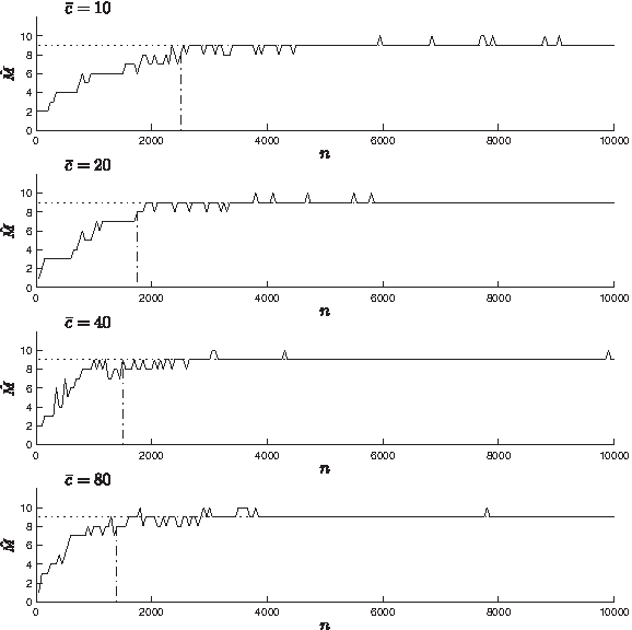
For each data set, with n ranging from 50 to 10,000 in increments of 50, we calculated \documentclass{aastex}\usepackage{amsbsy}\usepackage{amsfonts}\usepackage{amssymb}\usepackage{bm}\usepackage{mathrsfs}\usepackage{pifont}\usepackage{stmaryrd}\usepackage{textcomp}\usepackage{portland, xspace}\usepackage{amsmath, amsxtra}\pagestyle{empty}\DeclareMathSizes {10} {9} {7} {6}\begin{document}$$\boldsymbol{\hat M}$$\end{document} using the procedure described above; the results are shown in Figure 1. When there are very few columns, the best model is a simple one, with only one or two Dirichlet components. However, as the number of columns grows so, on average, does \documentclass{aastex}\usepackage{amsbsy}\usepackage{amsfonts}\usepackage{amssymb}\usepackage{bm}\usepackage{mathrsfs}\usepackage{pifont}\usepackage{stmaryrd}\usepackage{textcomp}\usepackage{portland, xspace}\usepackage{amsmath, amsxtra}\pagestyle{empty}\DeclareMathSizes {10} {9} {7} {6}\begin{document}$$\boldsymbol{\hat M}$$\end{document}, until it settles first into the range 9 ± 1, and eventually becomes nearly certain to equal 9, the number of components actually used to generate the data. For each data set, we indicate in Figure 1 the lowest value n′ for which \documentclass{aastex}\usepackage{amsbsy}\usepackage{amsfonts}\usepackage{amssymb}\usepackage{bm}\usepackage{mathrsfs}\usepackage{pifont}\usepackage{stmaryrd}\usepackage{textcomp}\usepackage{portland, xspace}\usepackage{amsmath, amsxtra}\pagestyle{empty}\DeclareMathSizes {10} {9} {7} {6}\begin{document}$$\boldsymbol{\hat M} = 9 \pm 1$$\end{document} for all tested n ≥ n′. The larger the average number of observations per column, the earlier this convergence tends to occur.
The estimated number of Dirichlet components as a function of data size. The 9-component DM \documentclass{aastex}\usepackage{amsbsy}\usepackage{amsfonts}\usepackage{amssymb}\usepackage{bm}\usepackage{mathrsfs}\usepackage{pifont}\usepackage{stmaryrd}\usepackage{textcomp}\usepackage{portland, xspace}\usepackage{amsmath, amsxtra}\pagestyle{empty}\DeclareMathSizes {10} {9} {7} {6}\begin{document}$${\tilde \theta}$$\end{document} was used to generate four data sets, with an average of \documentclass{aastex}\usepackage{amsbsy}\usepackage{amsfonts}\usepackage{amssymb}\usepackage{bm}\usepackage{mathrsfs}\usepackage{pifont}\usepackage{stmaryrd}\usepackage{textcomp}\usepackage{portland, xspace}\usepackage{amsmath, amsxtra}\pagestyle{empty}\DeclareMathSizes {10} {9} {7} {6}\begin{document}$${\bar c}$$\end{document} observations per column, with \documentclass{aastex}\usepackage{amsbsy}\usepackage{amsfonts}\usepackage{amssymb}\usepackage{bm}\usepackage{mathrsfs}\usepackage{pifont}\usepackage{stmaryrd}\usepackage{textcomp}\usepackage{portland, xspace}\usepackage{amsmath, amsxtra}\pagestyle{empty}\DeclareMathSizes {10} {9} {7} {6}\begin{document}$${\bar c} = 10, 20, 40$$\end{document}, and 80. Using our Gibbs-sampling algorithm applied to the first n columns of each data set (with n divisible by 50), and the MDL principle, we calculated \documentclass{aastex}\usepackage{amsbsy}\usepackage{amsfonts}\usepackage{amssymb}\usepackage{bm}\usepackage{mathrsfs}\usepackage{pifont}\usepackage{stmaryrd}\usepackage{textcomp}\usepackage{portland, xspace}\usepackage{amsmath, amsxtra}\pagestyle{empty}\DeclareMathSizes {10} {9} {7} {6}\begin{document}$$\boldsymbol{\hat M}$$\end{document}, the number of components in the optimal Dirichlet mixture model. For each data set, a vertical line indicates the the smallest n′ for which \documentclass{aastex}\usepackage{amsbsy}\usepackage{amsfonts}\usepackage{amssymb}\usepackage{bm}\usepackage{mathrsfs}\usepackage{pifont}\usepackage{stmaryrd}\usepackage{textcomp}\usepackage{portland, xspace}\usepackage{amsmath, amsxtra}\pagestyle{empty}\DeclareMathSizes {10} {9} {7} {6}\begin{document}$$\boldsymbol{\hat M} = 9 \pm 1$$\end{document} for all tested value of n ≥ n′.
Although the correct number of Dirichlet components can be recovered to good precision with even a relatively small number of columns, the recovery of accurate values for the parameters of the generating DM requires substantially more data. In Table 3, we compare the parameters recovered by the example considered in Table 2 to those of \documentclass{aastex}\usepackage{amsbsy}\usepackage{amsfonts}\usepackage{amssymb}\usepackage{bm}\usepackage{mathrsfs}\usepackage{pifont}\usepackage{stmaryrd}\usepackage{textcomp}\usepackage{portland, xspace}\usepackage{amsmath, amsxtra}\pagestyle{empty}\DeclareMathSizes {10} {9} {7} {6}\begin{document}$${\tilde \theta}$$\end{document}, used to generate the data. We also consider the parameters recovered using a much larger data set with n = 100,000 and \documentclass{aastex}\usepackage{amsbsy}\usepackage{amsfonts}\usepackage{amssymb}\usepackage{bm}\usepackage{mathrsfs}\usepackage{pifont}\usepackage{stmaryrd}\usepackage{textcomp}\usepackage{portland, xspace}\usepackage{amsmath, amsxtra}\pagestyle{empty}\DeclareMathSizes {10} {9} {7} {6}\begin{document}$${\bar c} = 80$$\end{document}, values which are comparable to those for real protein data sets used to derive DMs, such as that studied below. Given the larger data set, we are able to estimate both the mixture parameters \documentclass{aastex}\usepackage{amsbsy}\usepackage{amsfonts}\usepackage{amssymb}\usepackage{bm}\usepackage{mathrsfs}\usepackage{pifont}\usepackage{stmaryrd}\usepackage{textcomp}\usepackage{portland, xspace}\usepackage{amsmath, amsxtra}\pagestyle{empty}\DeclareMathSizes {10} {9} {7} {6}\begin{document}$${\tilde m}_i$$\end{document} and the concentration parameters \documentclass{aastex}\usepackage{amsbsy}\usepackage{amsfonts}\usepackage{amssymb}\usepackage{bm}\usepackage{mathrsfs}\usepackage{pifont}\usepackage{stmaryrd}\usepackage{textcomp}\usepackage{portland, xspace}\usepackage{amsmath, amsxtra}\pagestyle{empty}\DeclareMathSizes {10} {9} {7} {6}\begin{document}$$\alpha_i^*$$\end{document} on average to within 0.6%, and in no case to err by more than 1.5%. The smaller data set yields much larger errors, erring in the estimation of these parameters by over 15% more than half the time.
Comparison of Recovered to Generating DM Parameters
Using a nine-component DM \documentclass{aastex}\usepackage{amsbsy}\usepackage{amsfonts}\usepackage{amssymb}\usepackage{bm}\usepackage{mathrsfs}\usepackage{pifont}\usepackage{stmaryrd}\usepackage{textcomp}\usepackage{portland, xspace}\usepackage{amsmath, amsxtra}\pagestyle{empty}\DeclareMathSizes {10} {9} {7} {6}\begin{document}$${\tilde \theta}$$\end{document}, artificial data sets with (n = 2000, \documentclass{aastex}\usepackage{amsbsy}\usepackage{amsfonts}\usepackage{amssymb}\usepackage{bm}\usepackage{mathrsfs}\usepackage{pifont}\usepackage{stmaryrd}\usepackage{textcomp}\usepackage{portland, xspace}\usepackage{amsmath, amsxtra}\pagestyle{empty}\DeclareMathSizes {10} {9} {7} {6}\begin{document}$${\bar c} = 20$$\end{document}) and (n = 100, 000, \documentclass{aastex}\usepackage{amsbsy}\usepackage{amsfonts}\usepackage{amssymb}\usepackage{bm}\usepackage{mathrsfs}\usepackage{pifont}\usepackage{stmaryrd}\usepackage{textcomp}\usepackage{portland, xspace}\usepackage{amsmath, amsxtra}\pagestyle{empty}\DeclareMathSizes {10} {9} {7} {6}\begin{document}$${\bar c} = 80$$\end{document}) were generated. For each data set, a maximum-likelihood 9-component DM \documentclass{aastex}\usepackage{amsbsy}\usepackage{amsfonts}\usepackage{amssymb}\usepackage{bm}\usepackage{mathrsfs}\usepackage{pifont}\usepackage{stmaryrd}\usepackage{textcomp}\usepackage{portland, xspace}\usepackage{amsmath, amsxtra}\pagestyle{empty}\DeclareMathSizes {10} {9} {7} {6}\begin{document}$$\boldsymbol{\hat \theta}$$\end{document} was estimated. The parameters of each component i of \documentclass{aastex}\usepackage{amsbsy}\usepackage{amsfonts}\usepackage{amssymb}\usepackage{bm}\usepackage{mathrsfs}\usepackage{pifont}\usepackage{stmaryrd}\usepackage{textcomp}\usepackage{portland, xspace}\usepackage{amsmath, amsxtra}\pagestyle{empty}\DeclareMathSizes {10} {9} {7} {6}\begin{document}$${\tilde \theta}$$\end{document} are compared to the corresponding parameters in the nearest component of \documentclass{aastex}\usepackage{amsbsy}\usepackage{amsfonts}\usepackage{amssymb}\usepackage{bm}\usepackage{mathrsfs}\usepackage{pifont}\usepackage{stmaryrd}\usepackage{textcomp}\usepackage{portland, xspace}\usepackage{amsmath, amsxtra}\pagestyle{empty}\DeclareMathSizes {10} {9} {7} {6}\begin{document}$$\boldsymbol{\hat \theta}$$\end{document}. \documentclass{aastex}\usepackage{amsbsy}\usepackage{amsfonts}\usepackage{amssymb}\usepackage{bm}\usepackage{mathrsfs}\usepackage{pifont}\usepackage{stmaryrd}\usepackage{textcomp}\usepackage{portland, xspace}\usepackage{amsmath, amsxtra}\pagestyle{empty}\DeclareMathSizes {10} {9} {7} {6}\begin{document}$$JS (\boldsymbol{\tilde{\vec q}}_i, \boldsymbol{\hat{\vec q}}_i)$$\end{document} is the Jensen-Shannon divergence of the location parameter vectors \documentclass{aastex}\usepackage{amsbsy}\usepackage{amsfonts}\usepackage{amssymb}\usepackage{bm}\usepackage{mathrsfs}\usepackage{pifont}\usepackage{stmaryrd}\usepackage{textcomp}\usepackage{portland, xspace}\usepackage{amsmath, amsxtra}\pagestyle{empty}\DeclareMathSizes {10} {9} {7} {6}\begin{document}$$\boldsymbol{\tilde{\vec q}}_i$$\end{document} and \documentclass{aastex}\usepackage{amsbsy}\usepackage{amsfonts}\usepackage{amssymb}\usepackage{bm}\usepackage{mathrsfs}\usepackage{pifont}\usepackage{stmaryrd}\usepackage{textcomp}\usepackage{portland, xspace}\usepackage{amsmath, amsxtra}\pagestyle{empty}\DeclareMathSizes {10} {9} {7} {6}\begin{document}$$\boldsymbol{\hat {\vec q}}_i$$\end{document}, where \documentclass{aastex}\usepackage{amsbsy}\usepackage{amsfonts}\usepackage{amssymb}\usepackage{bm}\usepackage{mathrsfs}\usepackage{pifont}\usepackage{stmaryrd}\usepackage{textcomp}\usepackage{portland, xspace}\usepackage{amsmath, amsxtra}\pagestyle{empty}\DeclareMathSizes {10} {9} {7} {6}\begin{document}$$JS (\boldsymbol{\vec r}, \boldsymbol{\vec s})$$\end{document} is given by \documentclass{aastex}\usepackage{amsbsy}\usepackage{amsfonts}\usepackage{amssymb}\usepackage{bm}\usepackage{mathrsfs}\usepackage{pifont}\usepackage{stmaryrd}\usepackage{textcomp}\usepackage{portland, xspace}\usepackage{amsmath, amsxtra}\pagestyle{empty}\DeclareMathSizes {10} {9} {7} {6}\begin{document}$$\frac {1} {2} \sum\nolimits_{j} \left(r_j \ln \frac {2r_j} {r_j + s_j} + s_j \ln \frac {2s_j} {r_j + s_j} \right)$$\end{document}.
In general, the smaller \documentclass{aastex}\usepackage{amsbsy}\usepackage{amsfonts}\usepackage{amssymb}\usepackage{bm}\usepackage{mathrsfs}\usepackage{pifont}\usepackage{stmaryrd}\usepackage{textcomp}\usepackage{portland, xspace}\usepackage{amsmath, amsxtra}\pagestyle{empty}\DeclareMathSizes {10} {9} {7} {6}\begin{document}$$\boldsymbol{\tilde \alpha}_{i, j}$$\end{document}, the smaller the absolute but the greater the relative error in estimating its value, a fact related to the development in Ye et al. (2010). Thus, rather than recording data for individual \documentclass{aastex}\usepackage{amsbsy}\usepackage{amsfonts}\usepackage{amssymb}\usepackage{bm}\usepackage{mathrsfs}\usepackage{pifont}\usepackage{stmaryrd}\usepackage{textcomp}\usepackage{portland, xspace}\usepackage{amsmath, amsxtra}\pagestyle{empty}\DeclareMathSizes {10} {9} {7} {6}\begin{document}$$\boldsymbol{\tilde \alpha}_{i, j}$$\end{document}, Table 3 summarizes the accuracy with which each component's location parameters \documentclass{aastex}\usepackage{amsbsy}\usepackage{amsfonts}\usepackage{amssymb}\usepackage{bm}\usepackage{mathrsfs}\usepackage{pifont}\usepackage{stmaryrd}\usepackage{textcomp}\usepackage{portland, xspace}\usepackage{amsmath, amsxtra}\pagestyle{empty}\DeclareMathSizes {10} {9} {7} {6}\begin{document}$$\boldsymbol{\tilde{\vec q}}_i$$\end{document} are estimated, using the measure of Jensen-Shannon divergence. For the smaller data set, three of the components yield a divergence of over 0.025 bits, but for the larger data set the divergence in under 0.00025 bits for all but one component.
For the artificial data studied in this section, we made no attempt to improve the result for one value of M by using the best result for a neighboring value to select an initial θ. Averaged over 10 runs on an Intel Xeon 2.4-GHz E7440 CPU, using different random number seeds, our program took 1.7 seconds per run to converge for the (\documentclass{aastex}\usepackage{amsbsy}\usepackage{amsfonts}\usepackage{amssymb}\usepackage{bm}\usepackage{mathrsfs}\usepackage{pifont}\usepackage{stmaryrd}\usepackage{textcomp}\usepackage{portland, xspace}\usepackage{amsmath, amsxtra}\pagestyle{empty}\DeclareMathSizes {10} {9} {7} {6}\begin{document}$$n = 2000, {\bar c} = 20$$\end{document}) data set with M = 9, and 84 seconds for the (\documentclass{aastex}\usepackage{amsbsy}\usepackage{amsfonts}\usepackage{amssymb}\usepackage{bm}\usepackage{mathrsfs}\usepackage{pifont}\usepackage{stmaryrd}\usepackage{textcomp}\usepackage{portland, xspace}\usepackage{amsmath, amsxtra}\pagestyle{empty}\DeclareMathSizes {10} {9} {7} {6}\begin{document}$$n = 100000, {\bar c} = 80$$\end{document}) data set with M = 9.
A 9-component DM model provides 188 free parameters, and optimizing a function that yields local optima over a space of this size provides a significant challenge. Nevertheless, Table 3 suggests that when the observations are in fact generated by a DM contained in this model, our Gibbs-sampling algorithm is able to converge on the true solution given sufficient data.
5.2. Real data
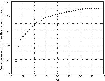
To analyze real data, we consider the “diverse-1216-uw” data set, from the website cited above, here called DUCSC, containing n = 314585 columns, with an average of \documentclass{aastex}\usepackage{amsbsy}\usepackage{amsfonts}\usepackage{amssymb}\usepackage{bm}\usepackage{mathrsfs}\usepackage{pifont}\usepackage{stmaryrd}\usepackage{textcomp}\usepackage{portland, xspace}\usepackage{amsmath, amsxtra}\pagestyle{empty}\DeclareMathSizes {10} {9} {7} {6}\begin{document}$${\bar c} = 75.99$$\end{document} amino acids per column, and the 20-component DM “dist.20comp,” here called θUCSC, that was previously derived from this data set. Letting θ0 be a multinomial distribution fit to the amino acid frequencies of DUCSC, a baseline description of the data has total description length \documentclass{aastex}\usepackage{amsbsy}\usepackage{amsfonts}\usepackage{amssymb}\usepackage{bm}\usepackage{mathrsfs}\usepackage{pifont}\usepackage{stmaryrd}\usepackage{textcomp}\usepackage{portland, xspace}\usepackage{amsmath, amsxtra}\pagestyle{empty}\DeclareMathSizes {10} {9} {7} {6}\begin{document}$${\rm DL} (D_{\rm UCSC} \mid \theta_0) + {\rm COMP} ({\cal M}_{20}, 314585 \times 75.99) = 99604971 + 206 = 99605177$$\end{document} bits, or 4.1667 bits per amino acid. Using θUCSC instead to describe the data, the total description length is reduced to \documentclass{aastex}\usepackage{amsbsy}\usepackage{amsfonts}\usepackage{amssymb}\usepackage{bm}\usepackage{mathrsfs}\usepackage{pifont}\usepackage{stmaryrd}\usepackage{textcomp}\usepackage{portland, xspace}\usepackage{amsmath, amsxtra}\pagestyle{empty}\DeclareMathSizes {10} {9} {7} {6}\begin{document}$${\rm DL} (D_{\rm UCSC} \mid \theta_{\rm UCSC}) + {\rm COMP} ({\cal DM}_{20, 20}, 314585, 75.99) = 74277770 + 3461 = 74281231$$\end{document} bits, or 3.1073 bits/a.a. The improvement with respect to the baseline multinomial model is 1.0594 bits/a.a., and is represented by a triangle in Figure 2.
Decrease in total description length as a function of the number of Dirichlet components. Given the data set DUCSC (with n = 314, 585 and \documentclass{aastex}\usepackage{amsbsy}\usepackage{amsfonts}\usepackage{amssymb}\usepackage{bm}\usepackage{mathrsfs}\usepackage{pifont}\usepackage{stmaryrd}\usepackage{textcomp}\usepackage{portland, xspace}\usepackage{amsmath, amsxtra}\pagestyle{empty}\DeclareMathSizes {10} {9} {7} {6}\begin{document}$${\bar c} = 75.99$$\end{document}), we used our Gibbs-sampling algorithm to estimate with θM the maximum-likelihood M-component DM, for M from 2 to 38. The total description length was calculated as \documentclass{aastex}\usepackage{amsbsy}\usepackage{amsfonts}\usepackage{amssymb}\usepackage{bm}\usepackage{mathrsfs}\usepackage{pifont}\usepackage{stmaryrd}\usepackage{textcomp}\usepackage{portland, xspace}\usepackage{amsmath, amsxtra}\pagestyle{empty}\DeclareMathSizes {10} {9} {7} {6}\begin{document}$${\rm DL} (D_{\rm UCSC} \mid \theta_M) + {\rm COMP} ({\cal DM}_{M, 20}, n, {\bar c})$$\end{document}, and compared to the total description length given the multinomial model on 20 letters, \documentclass{aastex}\usepackage{amsbsy}\usepackage{amsfonts}\usepackage{amssymb}\usepackage{bm}\usepackage{mathrsfs}\usepackage{pifont}\usepackage{stmaryrd}\usepackage{textcomp}\usepackage{portland, xspace}\usepackage{amsmath, amsxtra}\pagestyle{empty}\DeclareMathSizes {10} {9} {7} {6}\begin{document}$${\cal M}_20$$\end{document}. The decrease in description length per amino acid of the data is plotted, and reaches its maximum at \documentclass{aastex}\usepackage{amsbsy}\usepackage{amsfonts}\usepackage{amssymb}\usepackage{bm}\usepackage{mathrsfs}\usepackage{pifont}\usepackage{stmaryrd}\usepackage{textcomp}\usepackage{portland, xspace}\usepackage{amsmath, amsxtra}\pagestyle{empty}\DeclareMathSizes {10} {9} {7} {6}\begin{document}$$\boldsymbol{\hat M} = 35$$\end{document}. The triangle represents the decrease in description length yielded by the 20-component θUCSC, which was derived from DUCSC.
We applied the optimization methods described above to approximate maximum-likelihood θM for these data. In contrast to our artificial data, real data are not produced by a true underlying DM, even though they can perhaps be well modeled by one. This means that as the quantity of available data grows, the complexity of the best model is likely to grow as well, albeit slowly, never converging to a “true” number of components.
Because there is likely no true DM describing the data, the objective function tends to be much flatter over parameter space than it is for artificial data, making the search for a globally optimal DM correspondingly harder. Perhaps as a result, we found that for a given M, flat initial θs often were outperformed by initial θs derived from the best “current” solution for adjacent values of M. Thus, our optimization strategy consisted first of finding a set of provisional solutions θM for the range of M explored, and then of improving these solutions through further runs in which initial θs were derived from neighboring provisional θM.
We graph in Figure 2 the improvement in total description length our best θM yield with respect to the baseline, for M from 2 to 38. θ35 produced the greatest improvement, of 1.0654 bits/a.a. (On DUCSC, an average single run for M = 35 took 512 seconds until convergence.) θ16 yielded an improvement of 1.0595 bits/a.a., essentially equivalent to that of the 20-component θUCSC, and θ20 yielded the somewhat greater improvement of 1.0612 bits/a.a. Using the “fssp-3-5-98-select-0.8-3.cols” data set from the website above, we achieved comparable results and improvements with respect to the corresponding DM “fournier-fssp.20comp” (data not shown).
As is evident from Figure 2, until M = 35, increasing the number of components yields a steady but generally diminishing improvement in total description length. Programs that employ DMs generally run more slowly the larger the number of components, which provides an independent reason for preferring smaller M. There are no points in Figure 2 where the implicit slope changes abruptly, but examination suggests that for this data set, θ10, θ14, θ23, and θ29, which yield improvements that are, respectively, 99.0%, 99.3%, 99.7%, and 99.9% of the optimal, may provide good tradeoffs between simplicity and accurate description of the data.
6. Discussion
Although for real data, no optimal solution is known with certainty, it is instructive to examine the Dirichlet components recovered, and to compare θM for different values of M. In Table 4, we summarize the components of our θ10 and θ14, ordered by the magnitude of their mixture parameters mi. Similarly to the results of Brown et al. (1993) and Sjölander et al. (1996), most components can be seen to correspond to natural classes of amino acids. For example, component 9 of θ10 and component 13 of θ14 both favor the aromatic amino acids. Other components favor hydrophobic, positively charged, and negatively charged residues, and the special amino acids glycine and proline. It is also worth noting two other types of components. First, components 1 of θ10 and θ14 both have very low values of α*, indicating high probability density near the boundaries of multinomial space; the columns these components describe therefore consist heavily of single amino acids. As M grows further, a component of this type may break into multiple components, each with large α* and corresponding to a single amino acid, similar in this way to components 8 and 10 of θ10. Second, components 4 of θ10 and θ14 both have fairly high values of α*, but do not strongly favor or disfavor any amino acid. These components describe protein positions that are probably not under strong evolutionary pressure, and accept all amino acids at roughly their background frequencies.
The components of θ10 and θ14 are ordered by decreasing value of their mixture parameters \documentclass{aastex}\usepackage{amsbsy}\usepackage{amsfonts}\usepackage{amssymb}\usepackage{bm}\usepackage{mathrsfs}\usepackage{pifont}\usepackage{stmaryrd}\usepackage{textcomp}\usepackage{portland, xspace}\usepackage{amsmath, amsxtra}\pagestyle{empty}\DeclareMathSizes {10} {9} {7} {6}\begin{document}$$\boldsymbol{\vec m}$$\end{document}. For each component, the log ratio of each amino acid's location parameter to its background frequency is calculated, and listed in decreasing order of log ratio if this ratio is > 1, > 0.5 or < −1.
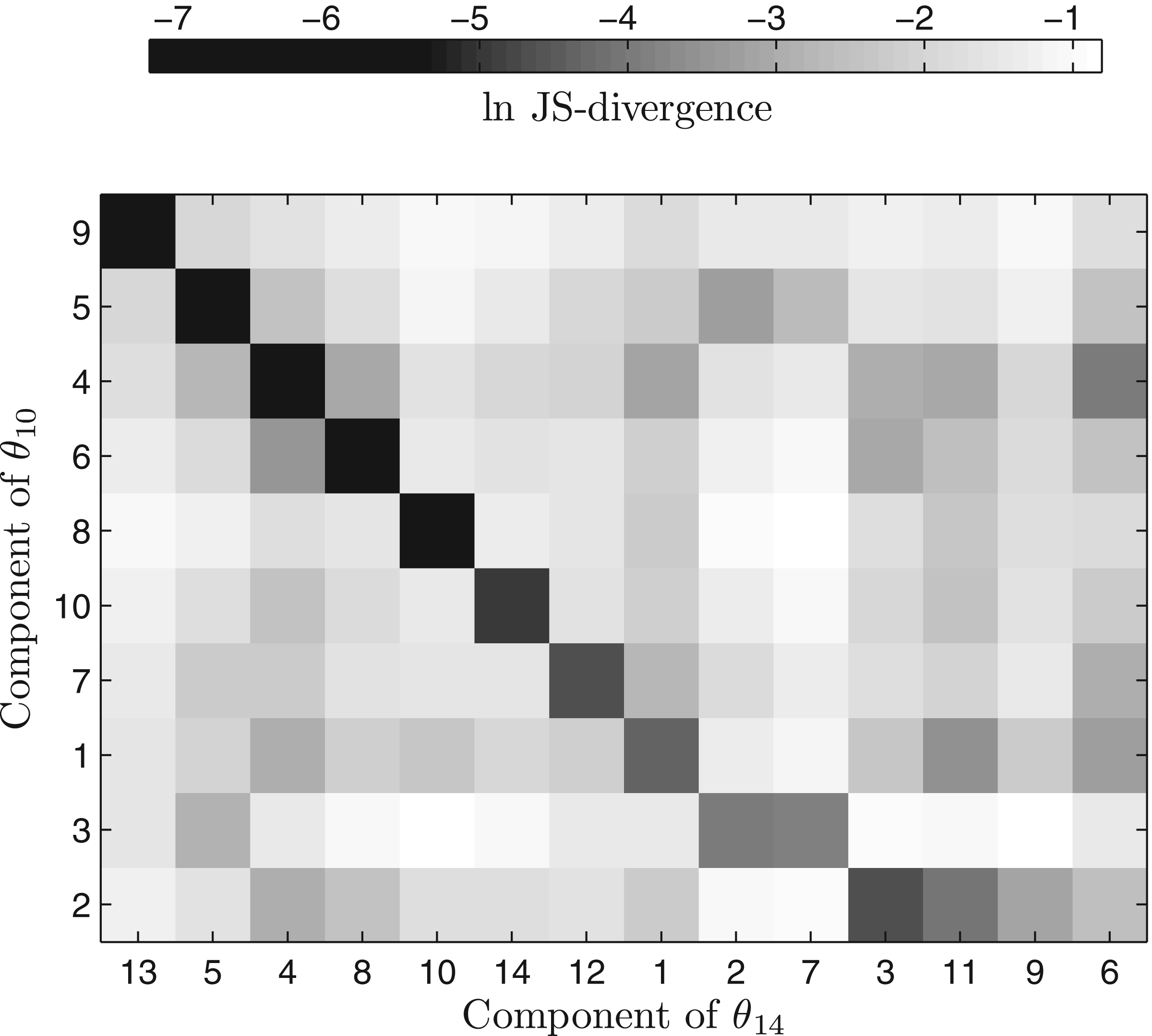
In Figure 3, we compare θ10's to θ14's location parameters. Qualitatively, it is evident that as M grows, many Dirichlet components retain their essential character, as represented by the corresponding components in the first eight rows and columns of the figure. Other Dirichlet components split apart, as seen in the last two rows, which correspond to components 3 and 2 of θ10 Finally, components of an almost completely new character can be born, as seen in the last two columns, which correspond to components 9 and 6 of θ14.
Comparison of location parameters for the Dirichlet mixtures θ10 and θ14. The location parameters \documentclass{aastex}\usepackage{amsbsy}\usepackage{amsfonts}\usepackage{amssymb}\usepackage{bm}\usepackage{mathrsfs}\usepackage{pifont}\usepackage{stmaryrd}\usepackage{textcomp}\usepackage{portland, xspace}\usepackage{amsmath, amsxtra}\pagestyle{empty}\DeclareMathSizes {10} {9} {7} {6}\begin{document}$$\boldsymbol{\vec q}_i$$\end{document} for each component of θ10 are compared to those for each component of θ14 using the measure of Jensen-Shannon divergence, described in the legend to Table 3. The indices of the components are those given in Table 4, and are reordered to make the relationships among components easier to read.
7. Conclusion
In this article, we have studied several questions relevant to the inference of a Dirichlet mixture model from a “gold standard” set of protein alignment data. We sought to apply the MDL principle to the question of how many components a Dirichlet mixture should have. This required an evaluation of the complexity of DM models, and we accordingly developed heuristic arguments for extending to Dirichlet mixtures an analytic formula for the complexity of a single Dirichlet model. A second element needed for the application of the MDL principle is a method for approximating maximum-likelihood DMs from a given set of data. Although this problem has been addressed previously, we have described a new Gibbs-sampling approach that reduces the high-dimensional optimization problem to several tractable one-dimensional optimization problems.
To test the efficacy of our methods, we have applied them to artificial data generated by a known Dirichlet mixture, and shown that they are able both to recover the correct number of Dirichlet components, and to converge effectively on the “true” DM parameters. Finally, we have applied our methods to real data, where they are able to recover DMs that describe the data more concisely than do DMs constructed using an earlier approach. It is hoped that the methods presented here will aid in the construction of improved DMs for the comparison of multiple protein sequences.
8. Appendix: Maximum-Likelihood Estimation of the Concentration Parameter
Our Gibbs sampling approach provides us with a way to estimate the values of the mixture parameters \documentclass{aastex}\usepackage{amsbsy}\usepackage{amsfonts}\usepackage{amssymb}\usepackage{bm}\usepackage{mathrsfs}\usepackage{pifont}\usepackage{stmaryrd}\usepackage{textcomp}\usepackage{portland, xspace}\usepackage{amsmath, amsxtra}\pagestyle{empty}\DeclareMathSizes {10} {9} {7} {6}\begin{document}$$\boldsymbol{\vec m}$$\end{document}, and thereby to reduce the problem of finding a maximum-likelihood (m.l.) Dirichlet mixture to that of finding a m.l. Dirichlet distribution. Because of this reduction, we simplify the notation in this section by dropping the component subscript i from all relevant parameters.
Let \documentclass{aastex}\usepackage{amsbsy}\usepackage{amsfonts}\usepackage{amssymb}\usepackage{bm}\usepackage{mathrsfs}\usepackage{pifont}\usepackage{stmaryrd}\usepackage{textcomp}\usepackage{portland, xspace}\usepackage{amsmath, amsxtra}\pagestyle{empty}\DeclareMathSizes {10} {9} {7} {6}\begin{document}$$\boldsymbol{\vec c}^{\, (k)}$$\end{document} be the letter count vectors associated with the n columns assigned to the bin in question, and let c*(k) be the total letter count for column k. Applying eq. (7), the log-likelihood \documentclass{aastex}\usepackage{amsbsy}\usepackage{amsfonts}\usepackage{amssymb}\usepackage{bm}\usepackage{mathrsfs}\usepackage{pifont}\usepackage{stmaryrd}\usepackage{textcomp}\usepackage{portland, xspace}\usepackage{amsmath, amsxtra}\pagestyle{empty}\DeclareMathSizes {10} {9} {7} {6}\begin{document}$${\cal L}$$\end{document} of the data is then given by
\documentclass{aastex}\usepackage{amsbsy}\usepackage{amsfonts}\usepackage{amssymb}\usepackage{bm}\usepackage{mathrsfs}\usepackage{pifont}\usepackage{stmaryrd}\usepackage{textcomp}\usepackage{portland, xspace}\usepackage{amsmath, amsxtra}\pagestyle{empty}\DeclareMathSizes {10} {9} {7} {6}\begin{document}\begin{align*}
{\cal L} & = \sum_ {k = 1} ^ {n} \ln \left[\frac {\Gamma
(\alpha^*)} {\Gamma (\alpha^* + c^ {* (k)})} \prod_ {j = 1} ^L
\frac {\Gamma (\alpha^* q_ {j} + c_j^ {(k)})} {\Gamma (\alpha^* q_
{j})} \right] \\ & = \sum_ {k = 1} ^ {n} \left\{\ln \Gamma
(\alpha^*) - \ln \Gamma (\alpha^* + c^ {* (k)}) + \sum_ {j = 1} ^L
\left[\ln \Gamma (\alpha^* q_ {j} + c_j^ {(k)}) - \ln \Gamma
(\alpha^* q_ {j}) \right] \right\}. \tag {8}
\end{align*}\end{document}
If the columns associated with a bin are assigned non-unitary weights wk, one may generalize this formula by simply including the factor wk before ln in the first summation.
Although it is possible to find the α* and \documentclass{aastex}\usepackage{amsbsy}\usepackage{amsfonts}\usepackage{amssymb}\usepackage{bm}\usepackage{mathrsfs}\usepackage{pifont}\usepackage{stmaryrd}\usepackage{textcomp}\usepackage{portland, xspace}\usepackage{amsmath, amsxtra}\pagestyle{empty}\DeclareMathSizes {10} {9} {7} {6}\begin{document}$$\boldsymbol{\vec q}$$\end{document} that maximize eq. (8) by Newton's method in L-dimensional space, the computation of the gradient and the Hessian matrix is time-consuming, especially when n is large. Thus, our second heuristic idea is to reduce the maximization problem to one dimension using first moment information from the \documentclass{aastex}\usepackage{amsbsy}\usepackage{amsfonts}\usepackage{amssymb}\usepackage{bm}\usepackage{mathrsfs}\usepackage{pifont}\usepackage{stmaryrd}\usepackage{textcomp}\usepackage{portland, xspace}\usepackage{amsmath, amsxtra}\pagestyle{empty}\DeclareMathSizes {10} {9} {7} {6}\begin{document}$$\boldsymbol{\vec c}^{\, (k)}$$\end{document}. In short, if \documentclass{aastex}\usepackage{amsbsy}\usepackage{amsfonts}\usepackage{amssymb}\usepackage{bm}\usepackage{mathrsfs}\usepackage{pifont}\usepackage{stmaryrd}\usepackage{textcomp}\usepackage{portland, xspace}\usepackage{amsmath, amsxtra}\pagestyle{empty}\DeclareMathSizes {10} {9} {7} {6}\begin{document}$$\boldsymbol{\vec p}$$\end{document} is sampled from a Dirichlet distribution with parameters \documentclass{aastex}\usepackage{amsbsy}\usepackage{amsfonts}\usepackage{amssymb}\usepackage{bm}\usepackage{mathrsfs}\usepackage{pifont}\usepackage{stmaryrd}\usepackage{textcomp}\usepackage{portland, xspace}\usepackage{amsmath, amsxtra}\pagestyle{empty}\DeclareMathSizes {10} {9} {7} {6}\begin{document}$$\boldsymbol{\vec \alpha}$$\end{document}, pj follows a beta distribution with parameters (αj, α* − αj). Furthermore, conditioning on c*(k) and pj, \documentclass{aastex}\usepackage{amsbsy}\usepackage{amsfonts}\usepackage{amssymb}\usepackage{bm}\usepackage{mathrsfs}\usepackage{pifont}\usepackage{stmaryrd}\usepackage{textcomp}\usepackage{portland, xspace}\usepackage{amsmath, amsxtra}\pagestyle{empty}\DeclareMathSizes {10} {9} {7} {6}\begin{document}$$c_j^{(k)}$$\end{document} follows a binomial distribution with parameters (c*(k), pj). This implies we can estimate qj by
\documentclass{aastex}\usepackage{amsbsy}\usepackage{amsfonts}\usepackage{amssymb}\usepackage{bm}\usepackage{mathrsfs}\usepackage{pifont}\usepackage{stmaryrd}\usepackage{textcomp}\usepackage{portland, xspace}\usepackage{amsmath, amsxtra}\pagestyle{empty}\DeclareMathSizes {10} {9} {7} {6}\begin{document}\begin{align*}
\boldsymbol{\hat q} _j = \frac {\sum_ {k = 1} ^n c_j^ {(k)}} {\sum_ {k = 1}
^n c^ {* (k)}}, \tag {9}
\end{align*}\end{document}
and replace qj in eq. (8) by \documentclass{aastex}\usepackage{amsbsy}\usepackage{amsfonts}\usepackage{amssymb}\usepackage{bm}\usepackage{mathrsfs}\usepackage{pifont}\usepackage{stmaryrd}\usepackage{textcomp}\usepackage{portland, xspace}\usepackage{amsmath, amsxtra}\pagestyle{empty}\DeclareMathSizes {10} {9} {7} {6}\begin{document}$$\boldsymbol{\hat q}_j$$\end{document}. This leaves the single parameter α* still to estimate.
where ψ and ψ′ are the digamma and trigamma functions. Given an initial α* near the m.l. \documentclass{aastex}\usepackage{amsbsy}\usepackage{amsfonts}\usepackage{amssymb}\usepackage{bm}\usepackage{mathrsfs}\usepackage{pifont}\usepackage{stmaryrd}\usepackage{textcomp}\usepackage{portland, xspace}\usepackage{amsmath, amsxtra}\pagestyle{empty}\DeclareMathSizes {10} {9} {7} {6}\begin{document}$$\boldsymbol{\tilde \alpha}^*$$\end{document} that optimizes \documentclass{aastex}\usepackage{amsbsy}\usepackage{amsfonts}\usepackage{amssymb}\usepackage{bm}\usepackage{mathrsfs}\usepackage{pifont}\usepackage{stmaryrd}\usepackage{textcomp}\usepackage{portland, xspace}\usepackage{amsmath, amsxtra}\pagestyle{empty}\DeclareMathSizes {10} {9} {7} {6}\begin{document}$${\cal L}$$\end{document}, it is then simple to estimate \documentclass{aastex}\usepackage{amsbsy}\usepackage{amsfonts}\usepackage{amssymb}\usepackage{bm}\usepackage{mathrsfs}\usepackage{pifont}\usepackage{stmaryrd}\usepackage{textcomp}\usepackage{portland, xspace}\usepackage{amsmath, amsxtra}\pagestyle{empty}\DeclareMathSizes {10} {9} {7} {6}\begin{document}$$\boldsymbol{\tilde \alpha}^*$$\end{document} to great precision in a small number of iterations using Newton's method. There are rapid algorithms for calculating ψ and ψ′ (Bernardo, 1976; Schneider, 1978; Spouge, 1994). Note as well that because ψ and ψ′ appear in eqs. (10) and (11) only as differences, they can be replaced by rational functions when all letter counts \documentclass{aastex}\usepackage{amsbsy}\usepackage{amsfonts}\usepackage{amssymb}\usepackage{bm}\usepackage{mathrsfs}\usepackage{pifont}\usepackage{stmaryrd}\usepackage{textcomp}\usepackage{portland, xspace}\usepackage{amsmath, amsxtra}\pagestyle{empty}\DeclareMathSizes {10} {9} {7} {6}\begin{document}$$c_j^{(k)}$$\end{document} are integral.
Several problem may arise with this approach. First, \documentclass{aastex}\usepackage{amsbsy}\usepackage{amsfonts}\usepackage{amssymb}\usepackage{bm}\usepackage{mathrsfs}\usepackage{pifont}\usepackage{stmaryrd}\usepackage{textcomp}\usepackage{portland, xspace}\usepackage{amsmath, amsxtra}\pagestyle{empty}\DeclareMathSizes {10} {9} {7} {6}\begin{document}$${\cal L}$$\end{document} may be maximized in the limit only at the boundaries of (0, ∞). One may show that \documentclass{aastex}\usepackage{amsbsy}\usepackage{amsfonts}\usepackage{amssymb}\usepackage{bm}\usepackage{mathrsfs}\usepackage{pifont}\usepackage{stmaryrd}\usepackage{textcomp}\usepackage{portland, xspace}\usepackage{amsmath, amsxtra}\pagestyle{empty}\DeclareMathSizes {10} {9} {7} {6}\begin{document}$${\cal L}$$\end{document} is optimal as α* approaches 0 only if each column of the data consists of a single type of letter, although this letter may vary from column to column (proof omitted). Furthermore, one may show that \documentclass{aastex}\usepackage{amsbsy}\usepackage{amsfonts}\usepackage{amssymb}\usepackage{bm}\usepackage{mathrsfs}\usepackage{pifont}\usepackage{stmaryrd}\usepackage{textcomp}\usepackage{portland, xspace}\usepackage{amsmath, amsxtra}\pagestyle{empty}\DeclareMathSizes {10} {9} {7} {6}\begin{document}$${\cal L}$$\end{document} is optimal as α* approaches ∞ only if the observed letter frequencies are identical from column to column (proof omitted). It is easy to detect and allow for these special cases, but when there are more than a very small number of columns associated with a bin they essentially never arise in practice. Second, it is possible that \documentclass{aastex}\usepackage{amsbsy}\usepackage{amsfonts}\usepackage{amssymb}\usepackage{bm}\usepackage{mathrsfs}\usepackage{pifont}\usepackage{stmaryrd}\usepackage{textcomp}\usepackage{portland, xspace}\usepackage{amsmath, amsxtra}\pagestyle{empty}\DeclareMathSizes {10} {9} {7} {6}\begin{document}$${\cal L}$$\end{document} has multiple local maxima over (0, ∞). We conjecture that this can not be the case, but have not been able to prove it. As shown by representative examples in Figure 4, \documentclass{aastex}\usepackage{amsbsy}\usepackage{amsfonts}\usepackage{amssymb}\usepackage{bm}\usepackage{mathrsfs}\usepackage{pifont}\usepackage{stmaryrd}\usepackage{textcomp}\usepackage{portland, xspace}\usepackage{amsmath, amsxtra}\pagestyle{empty}\DeclareMathSizes {10} {9} {7} {6}\begin{document}$${\cal L}$$\end{document} is very simply behaved in all cases we have observed. Third, it is possible that \documentclass{aastex}\usepackage{amsbsy}\usepackage{amsfonts}\usepackage{amssymb}\usepackage{bm}\usepackage{mathrsfs}\usepackage{pifont}\usepackage{stmaryrd}\usepackage{textcomp}\usepackage{portland, xspace}\usepackage{amsmath, amsxtra}\pagestyle{empty}\DeclareMathSizes {10} {9} {7} {6}\begin{document}$$d^2{\cal L} / d \alpha^{*2}$$\end{document} may be positive for an initial value of α*, for example if α* were chosen greater that 5.3 in panel B of Figure 4. It is trivial to detect such cases, and replace α* by a smaller value, for which \documentclass{aastex}\usepackage{amsbsy}\usepackage{amsfonts}\usepackage{amssymb}\usepackage{bm}\usepackage{mathrsfs}\usepackage{pifont}\usepackage{stmaryrd}\usepackage{textcomp}\usepackage{portland, xspace}\usepackage{amsmath, amsxtra}\pagestyle{empty}\DeclareMathSizes {10} {9} {7} {6}\begin{document}$$d^2{\cal L} / d \alpha^{*2}$$\end{document} is negative. In practice, as illustrated in Figure 4, we use the method of moments, detailed below, to initialize Newton's method. This approach yields initial α* that tend to be near to but somewhat smaller than the m.l. \documentclass{aastex}\usepackage{amsbsy}\usepackage{amsfonts}\usepackage{amssymb}\usepackage{bm}\usepackage{mathrsfs}\usepackage{pifont}\usepackage{stmaryrd}\usepackage{textcomp}\usepackage{portland, xspace}\usepackage{amsmath, amsxtra}\pagestyle{empty}\DeclareMathSizes {10} {9} {7} {6}\begin{document}$$\boldsymbol{\tilde \alpha}^*$$\end{document}.
The log-likelihood \documentclass{aastex}\usepackage{amsbsy}\usepackage{amsfonts}\usepackage{amssymb}\usepackage{bm}\usepackage{mathrsfs}\usepackage{pifont}\usepackage{stmaryrd}\usepackage{textcomp}\usepackage{portland, xspace}\usepackage{amsmath, amsxtra}\pagestyle{empty}\DeclareMathSizes {10} {9} {7} {6}\begin{document}$${\cal L}$$\end{document} of the data as a function of α*. The graphs give \documentclass{aastex}\usepackage{amsbsy}\usepackage{amsfonts}\usepackage{amssymb}\usepackage{bm}\usepackage{mathrsfs}\usepackage{pifont}\usepackage{stmaryrd}\usepackage{textcomp}\usepackage{portland, xspace}\usepackage{amsmath, amsxtra}\pagestyle{empty}\DeclareMathSizes {10} {9} {7} {6}\begin{document}$${\cal L}$$\end{document} in units of 106. Examples are shown for four bins generated using the data set DUCSC described in the text, with M = 10 components. (A) A bin generated after the first round of Gibbs sampling beginning from a flat initial θ; all 10 bins in this first round yield very similar results. (B) The bin corresponding to component 1 of Table 4, after convergence. (C) The bin corresponding to component 3 of Table 4, after convergence. (D) The bin corresponding to component 8 of Table 4, after convergence. Solid vertical lines indicate the maximum-likelihood values \documentclass{aastex}\usepackage{amsbsy}\usepackage{amsfonts}\usepackage{amssymb}\usepackage{bm}\usepackage{mathrsfs}\usepackage{pifont}\usepackage{stmaryrd}\usepackage{textcomp}\usepackage{portland, xspace}\usepackage{amsmath, amsxtra}\pagestyle{empty}\DeclareMathSizes {10} {9} {7} {6}\begin{document}$$\boldsymbol{\tilde \alpha}^*$$\end{document}. Dashed vertical lines indicate the \documentclass{aastex}\usepackage{amsbsy}\usepackage{amsfonts}\usepackage{amssymb}\usepackage{bm}\usepackage{mathrsfs}\usepackage{pifont}\usepackage{stmaryrd}\usepackage{textcomp}\usepackage{portland, xspace}\usepackage{amsmath, amsxtra}\pagestyle{empty}\DeclareMathSizes {10} {9} {7} {6}\begin{document}$$\boldsymbol{\hat \alpha}^*$$\end{document} calculated using the method of moments, and used to initiate Newton's method.
Just as we use first moment information for \documentclass{aastex}\usepackage{amsbsy}\usepackage{amsfonts}\usepackage{amssymb}\usepackage{bm}\usepackage{mathrsfs}\usepackage{pifont}\usepackage{stmaryrd}\usepackage{textcomp}\usepackage{portland, xspace}\usepackage{amsmath, amsxtra}\pagestyle{empty}\DeclareMathSizes {10} {9} {7} {6}\begin{document}$$\boldsymbol{\vec c}^{\, (k)}$$\end{document} to reduce the dimension of our problem, so we can use second moment information to obtain a starting point for Newton's method. Specifically, for an individual letter j, some algebra allows us to write a method-of-moments estimate of α* as
\documentclass{aastex}\usepackage{amsbsy}\usepackage{amsfonts}\usepackage{amssymb}\usepackage{bm}\usepackage{mathrsfs}\usepackage{pifont}\usepackage{stmaryrd}\usepackage{textcomp}\usepackage{portland, xspace}\usepackage{amsmath, amsxtra}\pagestyle{empty}\DeclareMathSizes {10} {9} {7} {6}\begin{document}
\begin{align*}
{\hat{\boldsymbol{\alpha}}}^* (j) = [\hat{\textbf{\textit q}}_j(1-\hat{\textbf{\textit q}}_j)
\frac{\hat{\textbf{E}}(c^{*2})}{\hat{\textbf{E}}^2(c^*)} - v_j] \ / \ [v_j -
\frac{\hat{\textbf{\textit q}}_j(1-\hat{\textbf{\textit
q}}_j)}{\hat{\textbf{E}}(c^*)}], \tag{12}
\end{align*}
\end{document}
This work was supported by the Intramural Research Program of the National Library of Medicine at the National Institutes of Health.
Disclosure Statement
No competing financial interests exist.
References
1.
AltschulS.F., GertzE.M., AgarwalaR.et al.2009. PSI-BLAST pseudocounts and the minimum description length principle. Nucleic Acids Res., 37:815–824.
2.
AltschulS.F., WoottonJ.C., ZaslavskyE.et al.2010. The construction and use of log-odds substitution scores for multiple sequence alignment. PLoS Comp. Biol., 6:e1000852.
3.
BernardoJ.M.1976. Algorithm AS 103: psi (digamma) function. J. R. Stat. Soc. Ser. C Appl. Stat., 25:315–317.
4.
BrownM., HugheyR., KroghA.et al.1993. Using Dirichlet mixture priors to derive hidden Markov models for protein families, 47–55. HunterL., SearlsD., ShavlikJ.Proc. First Int. Conf. Intell. Sys. Mol. Biol.AAAI Press: Menlo Park, CA.
5.
GemanS., GemanD.1984. Stochastic relaxation, Gibbs distributions, and the Bayesian restoration of images. IEEE Trans. Patt. Anal. Mach. Intell., 6:721–741.
6.
GrünwaldP.D.2007. The Minimum Description Length Principle. MIT Press: Cambridge, MA.
7.
KirkpatrickS., GelattC.D., VecchiM.P.1983. Optimization by simulated annealing. Science, 220:671–680.
8.
LawrenceC.E., AltschulS.F., BoguskiM.S.et al.1993. Detecting subtle sequence signals: a Gibbs sampling strategy for multiple alignment. Science, 262:208–214.
9.
MetropolisN., RosenbluthA.W., RosenbluthM. N.et al.1953. Equation of state calculations by fast computing machines. J. Chem. Phys., 21:1087–1092.
10.
SchneiderB. E.1978. Algorithm AS 121: trigamma function. J. R. Stat. Soc. Ser. C Appl. Stat., 27:97–99.
11.
SjölanderK., KarplusK., BrownM.et al.1996. Dirichlet mixtures: a method for improved detection of weak but significant protein sequence homology. Comput. Appl. Biosci., 12:327–345.
12.
SpougeJ.L.1994. Computation of the gamma, digamma, and trigamma functions. SIAM J. Numer. Anal., 31:931–944.
13.
YeX., YuY.-K., AltschulS. F.2010. Compositional adjustment of Dirichlet mixture priors. J. Comput. Biol., 17:1607–1620.
14.
YuY.-K., AltschulS. F.2011. The complexity of the Dirichlet model for multiple alignment data. J. Comput. Biol., 18(this issue).