
Abstract
Brain function is thought to emerge from the interactions among neuronal populations. Apart from traditional efforts to reproduce brain dynamics from the micro- to macroscopic scales, complementary approaches develop phenomenological models of lower complexity. Such macroscopic models typically generate only a few selected—ideally functionally relevant—aspects of the brain dynamics. Importantly, they often allow an understanding of the underlying mechanisms beyond computational reproduction. Adding detail to these models will widen their ability to reproduce a broader range of dynamic features of the brain. For instance, such models allow for the exploration of consequences of focal and distributed pathological changes in the system, enabling us to identify and develop approaches to counteract those unfavorable processes. Toward this end, The Virtual Brain (TVB) (
Introduction
C
In this article, we describe a newly developed neuroinformatics platform—The Virtual Brain (TVB;
Model-based multimodal data integration approaches have many advantages over conventional approaches such as direct data fusion or converging evidence (Horwitz and Poeppel, 2002; Valdes-Sosa et al., 2009). Direct data fusion aims for the direct comparison of data sets from different imaging modalities using mathematical or statistical assessment criteria. However, these approaches often rest on the assumption of identical neuronal signal generators or that signals from different modalities have compatible features. The signals of the spatiotemporal source activity patterns do not necessarily need to overlap in different modalities nor do high statistical correlations between activation levels need to point to the true site of the signal source (Schulz et al., 2004). Model-based approaches, on the other hand, are able to integrate information from different modalities in a complementary manner, while avoiding limitations arising from pure statistical comparisons that do not incorporate structural and dynamical knowledge about the distinct underlying neurophysiological sources that generate the respective signals. Thus, in our view, the most reasonable way to integrate multimodal neuroimaging data together with existing knowledge about brain functioning and physiology is by means of a computational model that describes the emergence of high-level phenomena on the basis of basic bottom-up interaction between the elementary brain-processing units.
Large-scale neural network models can be built to incorporate prior knowledge about brain physiology and can be combined with forward models that allow the simulation of neuroimaging modalities (e.g., fMRI and EEG). This approach promotes the direct formulation and evaluation of hypotheses on how cognitive processes are generated by neuronal interaction. This can take the form of specific features of the model network structure, that is, interaction strength and delay between neural elements, or biophysical properties such as resting potentials, membrane permeability, plasticity effects, and so on. The data generated by these models can be directly compared to the signals from the respective imaging modality, and model parameters can be adjusted to the observed data. In an iterative manner, the fit between model output and empirical data is evaluated and used to improve the unobservable model components such as parameter settings or the model structure itself. The careful selection of local mesoscopic models and the iterative refinement of model network structure and parameter optimization lead to systematic improvements in model validity and thereby in knowledge about brain physiology and mechanisms underlying cognitive processing. Cognitive and behavioral experiments can then be interpreted in the light of model behavior that directly points to the underlying neuronal processes. For example, analyzing the variation of parameter settings in response to experimental conditions can deliver insights on the role of the associated structural or dynamical aspects in a certain cognitive function. Further, the relevance of neurobiological features for the emergence of self-organized criticality and neuronal information processing can be tested.
In summary, the model-based nexus of experimental and theoretical evidence allows the systematic inference of determinants of the generation of neuronal dynamics. Model-based integration of different neuroimaging modalities enables the exploration of consequences of biophysically relevant parameter changes in the system as they occur in changing brain states or during pathology. Hence, TVB helps us to uncover (1) the fundamental neuronal mechanisms that give rise to typical features of brain dynamics and (2) how intersubject variability in the brain structure results in differential brain dynamics.
The purpose of this article was to describe the main concept and to provide the proof of principle based on empirical data and example simulations. The article is structured as follows:
In the first section Modeling Large-Scale Brain Dynamics, we describe the principles governing the construction of large-scale brain models in TVB. This includes a description of the neuronal source model and the forward models used to translate the signals from individual sources into brain imaging signals. We describe the local mesoscopic models representing the local dynamics of the brain regions as well as the anatomical connectivity constraints coming from tract length, capacity, and directionality. Finally, we describe how the mean field activity is translated into signals that are comparable to the brain-imaging methods such as EEG and fMRI.
Next, in the section Identification of Spatiotemporal Motifs, we describe the proposed steps for the integration of functional empirical and simulated data. This includes deriving spatial register between data sets and reducing the parameter space to minimize the computation time. We detail our employed parameter estimation algorithm and discuss the possibilities provided by Building a dictionary of dynamical regimes, which lists the collection of parameter settings that produce different large-scale dynamics.
Finally, in the section Benefits of TVB Platform, we discuss examples how TVB can be used to obtain insights into brain function that could not be obtained by either empirical or theoretical approaches alone and help formulating new testable hypotheses.
Modeling Large-Scale Brain Dynamics
A choice of local mesoscopic dynamics
The brain contains ∼1011 neurons linked by ∼1015 connections, with each neuron having inputs in the order of 105. The complex and highly nonlinear neuronal interaction patterns are only poorly understood, and the number of degrees of freedom of a microscopic model attempting to describe every neuron, every connection, and every interaction is astronomically large and therefore far too high for fitting it directly with the recorded macroscopic data. The gap between the microscopic sources of scalp potentials at the cell membranes and the recorded macroscopic potentials can be bridged by an intermediate mesoscopic description (Nunez and Silberstein, 2000). Mesoscopic dynamics describe the activity of populations of neurons organized as cortical columns or subcortical nuclei. Several features of mesoscopic and macroscopic electric behavior, for example, dynamic patterns such as synchrony of oscillations or evoked potentials, show good correspondence to certain cognitive functions, for example, resting-state activity, sleep patterns, or event-related activity.
Common assumptions in the neural mass or mean-field modeling are that explicit structural features or temporal details of neuronal networks (e.g., spiking dynamics of single neurons) are irrelevant for the analysis of complex mesoscopic dynamics, and the emergent collective behavior is only weakly sensitive to the details of individual neuron behavior (Breakspear and Jirsa, 2007). Basic mean field models capture changes of the mean firing rate (Brunel and Wang, 2003), whereas more sophisticated mean field models account for parameter dispersion in the neurons and the subsequent richer behavioral repertoire of the mean field dynamics (Assisi et al., 2005; Jirsa and Stefanescu, 2011; Stefanescu and Jirsa, 2008, 2011). These approaches demonstrate a relatively new concept from statistical physics that macroscopic physical systems obey laws that are independent of the details of the microscopic constituents they are built of (Haken, 1975). These and related ideas have been exploited in neurosciences (Buzsaki, 2006; Kelso, 1995). Thus, our main interest lies in deriving the mesoscopic laws that drive the observed dynamical processes at the macroscopic scale in a systematic manner.
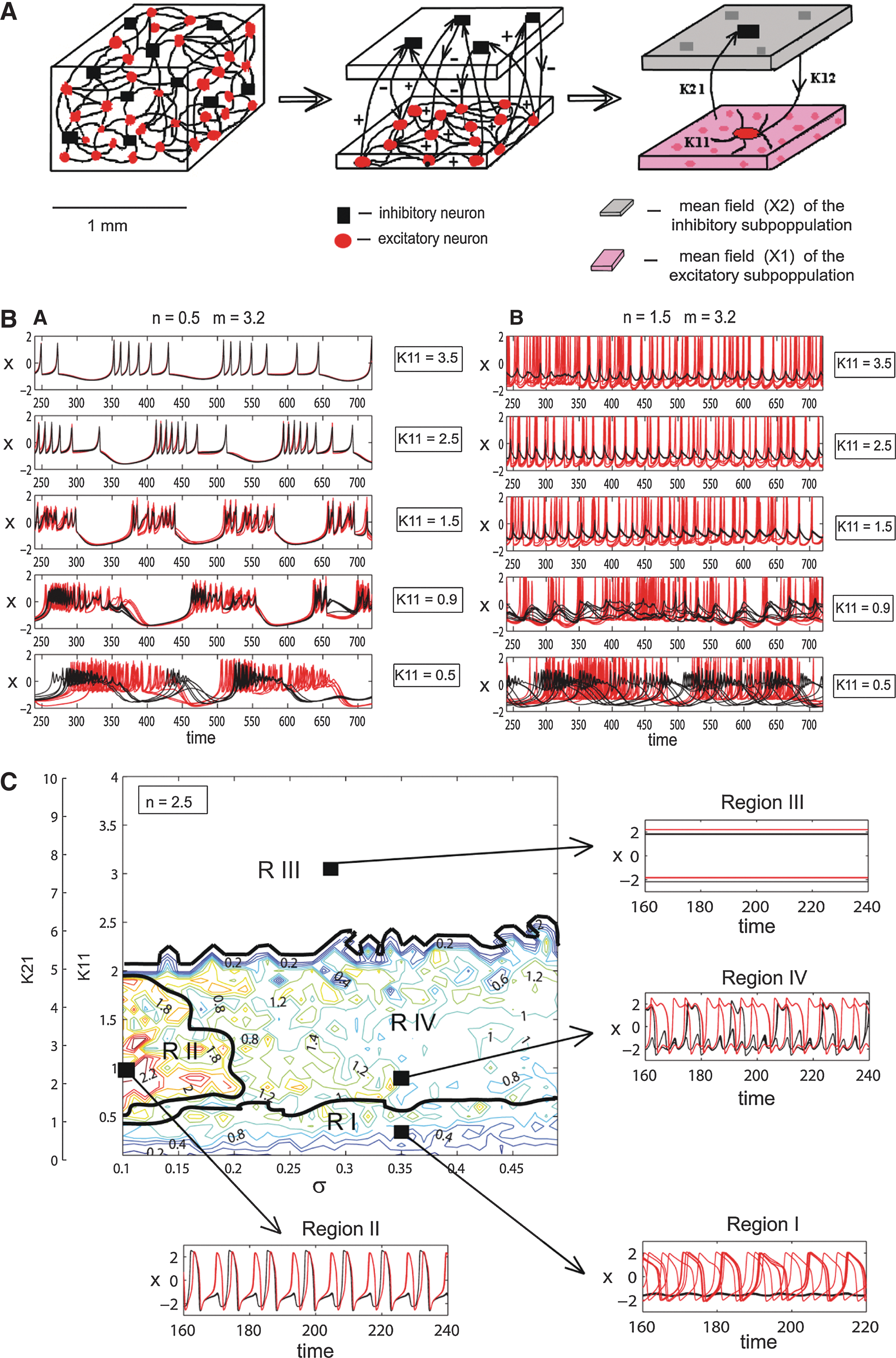
In the framework of TVB, we incorporate biologically realistic large-scale coupling of neural populations at salient brain regions that is mediated by long-range neural fiber tracts as identified with diffusion tensor imaging (DTI)-based tractography together with mean-field models as local node models. Various mean-field models are available in TVB, reproducing typical features of the mesoscopic population dynamics. For the simulations in present work, we use the Stefanescu–Jirsa model (2008) that is based on mean-field dynamics of a heterogeneous network of Hindmarsh–Rose neurons capable of displaying various spiking and bursting behaviors.
The Stefanescu–Jirsa neural population model provides a low-dimensional description of complex neural population dynamics, including synchronization and random firings of neurons, multiclustered behaviors, bursting, and oscillator death. The conditions under which these behaviors occur are shaped by specific parameter settings, including, for example, connectivity strengths and neuronal membrane excitability. A characteristic feature of the Stefanescu–Jirsa model is that it takes into account the parameter dispersion (i.e., nonidentical neurons in the population), giving rise to a rich repertoire of behaviors.
A neural population model
Since the reduced system is composed of three components or modes, each variable and parameter is either a column vector with three rows or a 3×3 square matrix:
This dynamical system describes the state evolution of two coupled populations of excitatory (variables x, y, and z) and inhibitory neurons (variables w, v, and u). In its original single-neuron formulation—that is known for its good reproduction of burst and spike activity and other empirically observed patterns—the variable x(t) encodes the neuron membrane potential at time t, while y(t) and z(t) account for the transport of ions across the membrane through ion channels. The spiking variable y(t) accounts for the flux of sodium and potassium through fast channels, while z(t), called bursting variable, accounts for the inward current through slow-ion channels (Hindmarsh and Rose, 1984). Even if it is not justified to directly expand this interpretation of variables and parameters from the single-neuron formulation to an analogous comprehension of their mean-field counterparts, the mean-field terms are nevertheless related to some of the underlying biophysical properties of the system [see Stefanescu and Jirsa (2008)]. Several biophysical parameters are permanently subject to ongoing fluctuations that are directly related to qualitative changes in the dynamics of the network. It is noteworthy that the mathematical structure of the single-neuron model is reflected in the mathematical structure of the population model. The population parameters comprise the contributions of the couplings and the distribution of the parameters.
Each of the three modes of the Stefanescu–Jirsa model (Eq. 1) reflects distinct dynamical behaviors depending on the range of membrane excitabilities of the neuron cluster (Stefanescu and Jirsa, 2008).
Full-brain model: coupling mesoscopic models with individual connectivity features
When traversing the scale to the large-scale network, population dynamics described by Equation 1 are connected using DTI tractography-derived coupling parameters. Each node of the large-scale network is now governed by its own intrinsic dynamics generated by the six equations and the dynamics of the coupled nodes that is summed to the local mean-field potential xi
. This yields the following evolution equation for the time course
The equation describes the numerical integration of a network of N connected neural populations
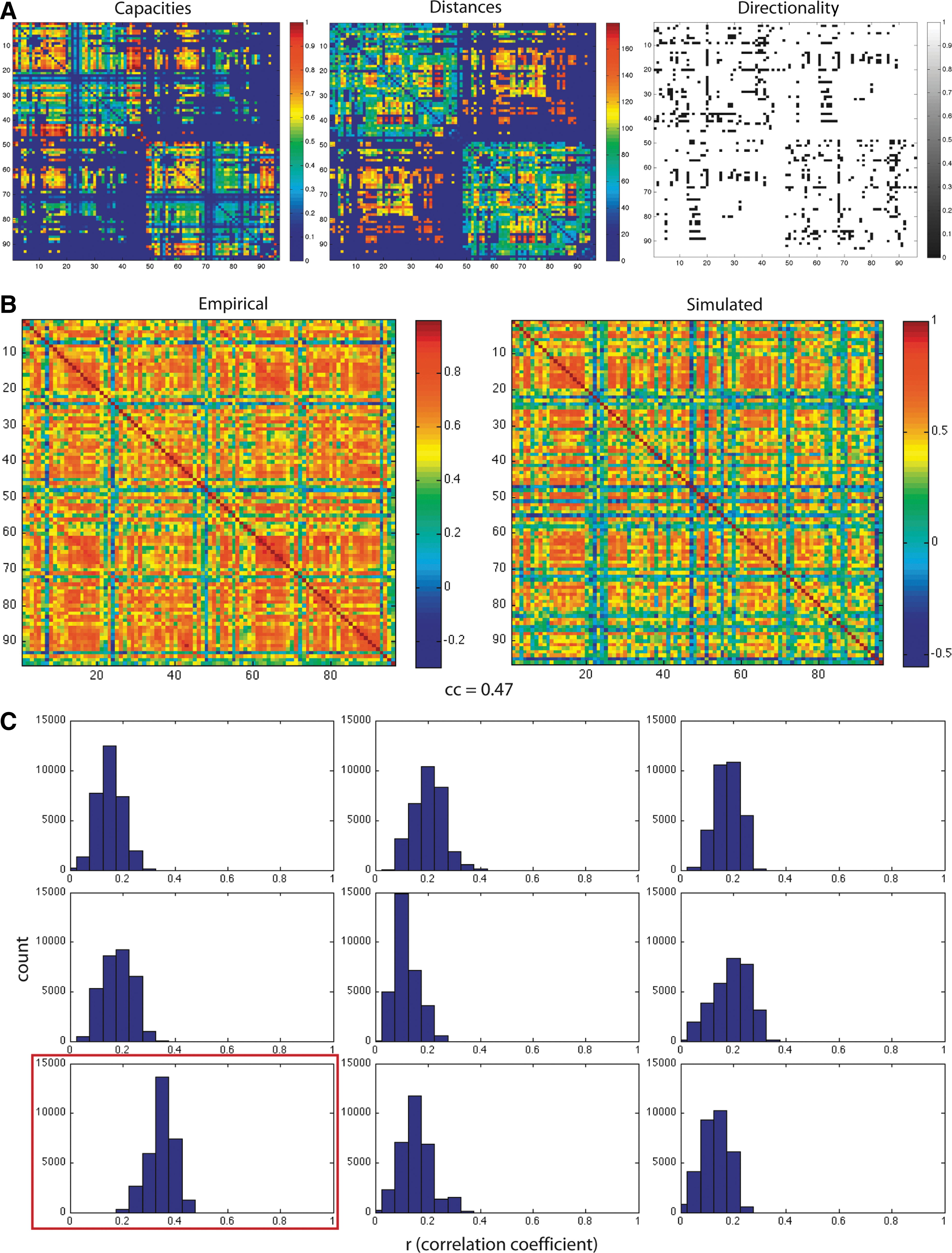
The order of names represents the order of nodes in the connectivity matrices depicted throughout the article.
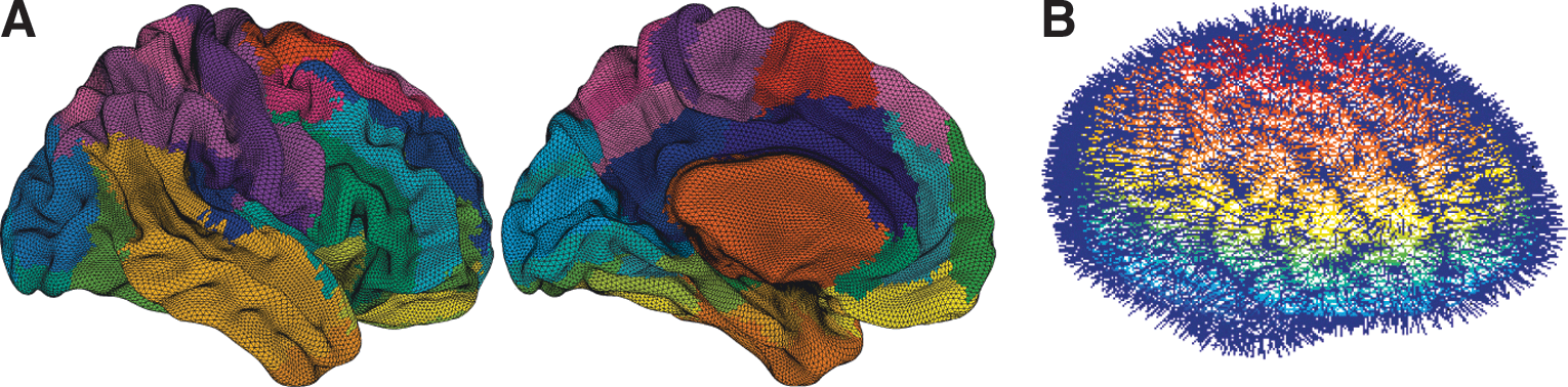
The brain connectivity of TVB distinguishes region-based and surface-based connectivity. In the former case, the networks comprise discrete nodes and connectivity, in which each node models the neural population activity of a brain region, and the connectivity is composed of inter-regional fibers. Region-based networks contain typically 30–200 network nodes. In the latter case, the cortical and subcortical areas are modeled on a finer scale by 5000–150,000 points, in which each point represents a neural population model. This approach allows a detailed spatial sampling, in particular, of the cortical surface, resulting in a spatially continuous approximation of the neural activity known as neural field modeling (Amari, 1977; Jirsa and Haken, 1996; Nunez, 1974; Robinson, 1997; Wilson-Cowan, 1972). Here, the connectivity is composed of local intracortical and global intercortical fibers.
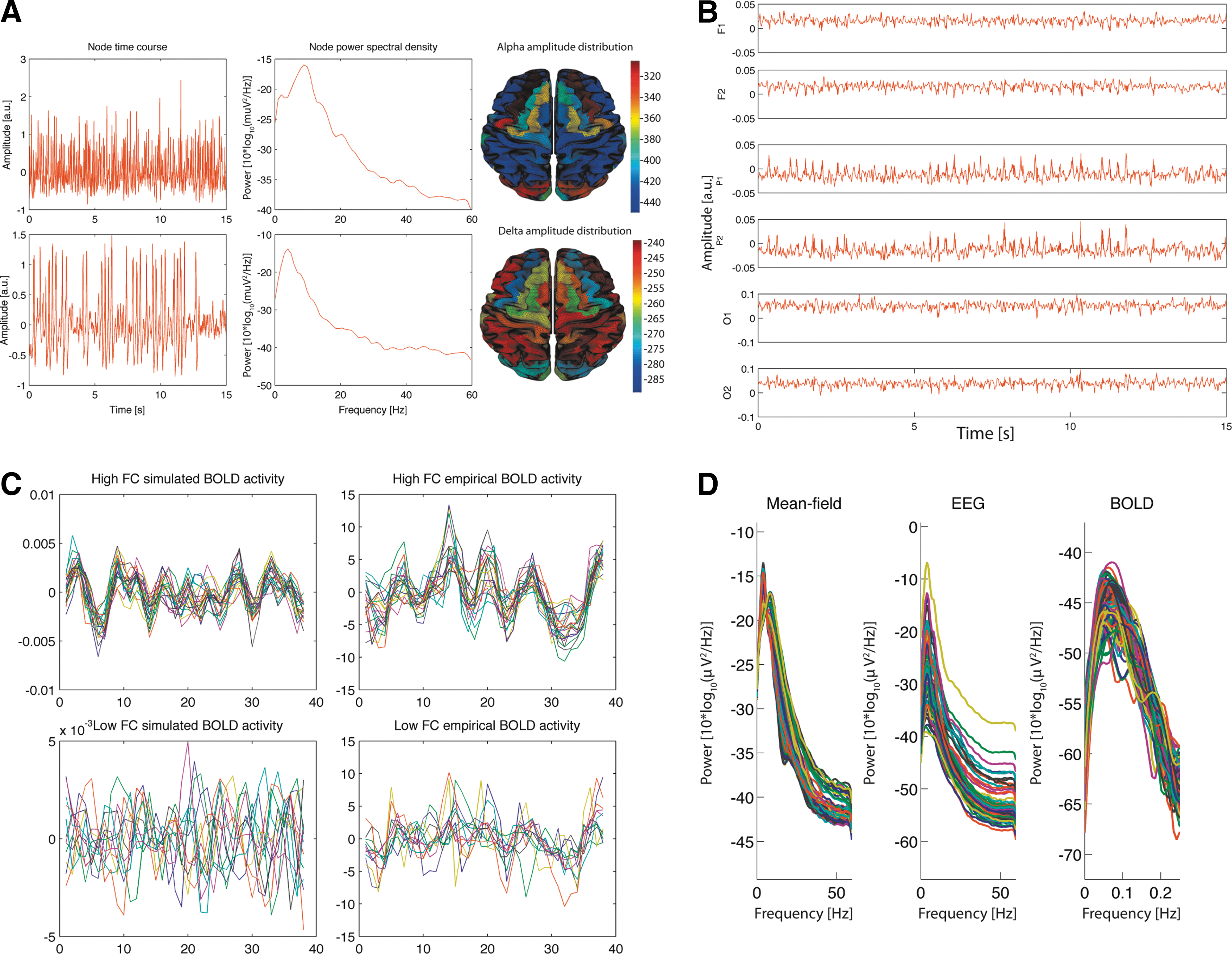
An example of the mean-field potential of two different brain areas as generated by the Stefanescu-Jirsa model is given in Figure 3A. As visible in the power spectral densities (PSD) next to the traces the upper mean-field potential has a spectral peak in the alpha band, while the lower one is dominated by delta activity. Figure 3B shows 15 seconds of simulated EEG activity for a selection of six channels. In Figure 3C a comparison of simulated and empirical BOLD activity (average over region-voxels) for low and high functional connectivity is shown. Figure 3D compares PSD of simulated mean-field source, EEG and BOLD activity.
Forward model
Upon simulating brain activity in the simulator core of TVB, the generated neural source activity time courses from both region- and surface-based approaches are projected into EEG, MEG, and blood oxygen level-dependent (BOLD) contrast space using a forward model (Bojak et al., 2010). The first neuroinformatic integration of these elements has been performed by Jirsa and colleagues (2002) demonstrating neural field modeling in an event-related paradigm. Homogeneous connectivity along the lines of Jirsa and Haken (1996) was implemented. Neural field activity was simulated on a spherical surface for computational efficiency and then mapped upon the convoluted cortical surface with its gyri and sulci. The forward solutions of EEG and MEG signals showed that a surprisingly rich complexity is observable in the EEG and MEG space, despite simplicity in the neural field dynamics. In particular, neural field models (Amari, 1978; Jirsa and Haken, 1996; Nunez, 1974 Robinson, 1997; Wilson-Cowan, 1974) have a spatial symmetry in their connectivity, which is always reflected in the symmetry of the resulting neural source activations, even though it may be significantly less apparent (if at all) in the EEG and MEG space. This led to the conclusion that the integration of tractographic data is imperative for future large-scale brain modeling attempts (Jirsa et al., 2002), since the symmetry of the connectivity will constrain the solutions of the neural sources.
Computing EEG/MEG signals
The forward problem of the EEG and MEG is the calculation of the electric potential V(x) on the skull and the magnetic field B(x) outside the head from a given primary current distribution D(x,t) as described by Jirsa and colleagues (2002) which we summarize in the following. The sources of the electric and magnetic fields are both primary and return currents. The situation is complicated by the fact that the present conductivities such as the brain tissue and the skull differ by the order of 100. Three-compartment volume conductor models are constructed from structural MRI data; the surfaces for the interfaces between the gray matter, cerebrospinal fluid, and white matter are approximated with triangular meshes (see Fig. 4). For EEG predictions, volume conduction models for the skull and scalp surfaces are incorporated. Here it is assumed that the electric source activity can be well approximated by the fluctuation of equivalent current dipoles generated by excitatory neurons that have dendritic trees oriented roughly perpendicular to the cortical surface and that constitute the majority of neuronal cells (∼85% of all neurons). We neglect dipole contributions from inhibitory neurons, since they are only present in a low number (∼15%), and their dendrites fan out spherically. Therefore, dipole strength can be assumed to be roughly proportional to the average membrane potential of the excitatory population (Bojak et al., 2010).
EEG forward modeling—calculating the EEG channel signals yielded by the neuronal source activity at the cortical nodes.
Dipole locations are assumed to be identical to source locations used for DTI tractography, while orientations are inferred as the normal of the triangulations of the segmented anatomical MR images (Fig. 4). Besides amplitude, every dipole has six additional degrees of freedom necessary for describing its position and orientation within the cortical tissue. At this stage, we have a representation of the current distribution in the three-dimensional physical space
The current density
where
Following the lines of Hamalainen et al. (1989, 1993) and using the Ampere–Laplace law, the forward MEG solution is obtained by the volume integral
where dν′ is the volume element,
The forward EEG solution is given by the boundary problem
which is to be solved numerically for an arbitrary head shape, typically using boundary element techniques as presented by Hamalainen (1992) and Nunez and Srinivasan (2006). In particular, these authors showed that for the computation of neuromagnetic and neuroelectric fields arising from cortical sources, it is sufficient to replace the skull by a perfect insulator, and, therefore, to model the head as a bounded brain-shaped homogeneous conductor. Three surfaces S 1 S 2 S 3 have to be considered at the scalp–air, the skull–scalp, and the skull–brain interface, respectively, whereas the latter provides the major contribution to the return currents. The three-dimensional geometry of these surfaces is obtained from MRI scans. There are various methods to solve the boundary problem above [see for instance, Hamalainen (1992) and Oostendorp et al. (2000)], but all of them compute some form of a transfer matrix acting upon the distributed neural sources and providing the forward EEG at electrode locations. The boundary-element (BEM) models are based on meshes that form a closed triangulation of the compartment surfaces from segmented T1-weighed MRI surfaces. Finite element method models consist of multiple tetrahedra, allowing to model tissue anisotropy that is physiologically more realistic at the cost of computational resources.
In the current study, we used the software packages spm8 (
EEG signals can now be calculated by applying the resulting LFM to the mean field source activity generated by the Stefanescu–Jirsa model (example shown in Fig. 3B). The corresponding frequency spectrum of the thus generated EEG is shown in Figure 3D.
Computing fMRI BOLD signals
Subsequent to the fitting of electric activity with the model, we want to compare model predictions of BOLD contrast with actual recorded fMRI timeseries data to deduce and integrate further constrains from and into the model and to perform analyses on the coupling between neural activity and BOLD contrast fluctuation.
Yet, the relation between neuronal activity and the BOLD signal is far from being elucidated (Bojak et al., 2010). Some major questions are not yet sufficiently answered, such as which neuronal and glial processes contribute to the BOLD signal? Via which molecular mechanisms do they influence the BOLD signal? What are the precise space–time properties of such a neurohemodynamic coupling?
Empirical and theoretical evidence indicates that different types of neuronal processes, such as action potentials, synaptic transmission, neurotransmitter cycling, and cytoskeletal turnover, have differential effects on the BOLD signal. For example, synaptic transmission and transmitter cycling are associated with higher metabolic demands than the conduction of action potentials (Attwell and Laughlin, 2001; Creutzfeldt et al., 1975; Dunning and Wolff, 1937). This is in line with a study showing a tighter relation of the BOLD signal to local field potentials that mainly represent postsynaptic potentials than to single- and multiunit activity, which represents action potentials (Logothetis et al., 2001). With respect to the molecular mechanism, the excitatory neurotransmitter glutamate has been shown to be a major modulator of the BOLD signal (Giaume et al., 2010; Petzold et al., 2008). Due to conflicting findings, there is a longstanding debate whether and if so how inhibitory neuronal activity can be detected by fMRI (Ritter et al., 2002). The issue gets complicated since likely multiple effects contribute at varying degrees in different brain regions and under different conditions (Iadecola, 2004).
The temporal properties of blood oxygenation/BOLD signal changes are modeled by either convolution of the approximated neuronal activity with the canonical hemodynamic response function assuming neurohemodynamic coupling to be linear and time invariant (Wobst et al., 2001), using a parametric set of response functions to account for variations in coupling and for nonlinearities (Friston et al., 1998), or by using the more elaborated biophysical hemodynamic model referred to as the Ballon–Windkessel model (Buxton et al., 1998; Friston et al., 2000, 2003; Mandeville et al., 1999). The latter approach is a state model with four state variables: synaptic activity, flow, volume, and deoxygenated hemoglobin. It assumes a three-stage coupling cascade: (1) a linear coupling between synaptic activity and blood flow; (2) a nonlinear coupling between blood flow and blood oxygenation and blood volume due the elastic properties of the venous vessels—hence, the name Ballon–Windkessel model; and (3) a nonlinear transformation of the variable flow and volume into the BOLD signal (Friston et al., 2003).
In a full-brain model comprising oscillators that in contrast to the here used Stefanescu–Jirsa model were less biophysically founded, local neural activity was approximated as the derivative of the state variable and used as an input for a neurohemodynamic coupling model (Ghosh et al., 2008). Approaches that are based on spiking neuron models use firing rates as input for BOLD signal estimation. Authors motivated that by the fact that in most cases, the firing rate is well correlated with excitatory synaptic activity (Deco and Jirsa, 2012). In the present study, however, the Stefanescu-Jirsa model provides six state variables with different biophysical counterparts; futhermore, each of them is described by the sum of the activity of three modes which model the activity of different neuronal subclusters of the inhibitory and the excitatory populations. For the simulated BOLD data shown here, we follow the line of Bojak and colleagues (2010) in assuming that BOLD contrast is primarily modulated by glutamate release. Hence, we approximate the BOLD signal time courses from the mean fields of the excitatory populations at each node. The mean-field amplitude time courses are convolved with a canonical hemodynamic response function as included in the SPM software package (
In Figure 3C, we show the approximated BOLD signal dynamics for regions of interest (ROIs) that exhibit high and low functional connectivity (FC). In Figure 3C, we also show empirical BOLD signal time courses extracted from the same cortical nodes by averaging the BOLD signal over all voxels contained by the respective ROI.
The frequency spectrum in Figure 3D indicates that the simulated BOLD signals exhibit peak frequencies below 0.1 Hz; that is, they exhibit the typical low-frequency oscillations reported previously for the resting-state BOLD signal.
There is potential for further advancement of the neurohemodynamic model, for example, by including assumptions about how astrocytes mediate the signal from neurons that cause dilatation of arterioles and resulting increase in blood flow considering the finite range of astrocyte projections (Drysdale et al., 2010). It is pointed out by the authors of this article that the distribution of effective connectivity between neurons and flow regulation points has not been measured experimentally yet, but is an area of active research interest [see also Aquino and associates (2012)]. Incorporating more details on the spatiotemporal aspects of neurohemodynamic coupling would considerably increase the value of the BOLD signal in model identification.
Identification of Spatiotemporal Motifs
Fitting computational models with actual recorded neuroimaging data requires several methodological considerations. Fitting the model with short epochs of empirical EEG-fMRI data yields individual model instances (parameter values). Thereby, we determine parameter values that are related to particular features of the recorded EEG-fMRI timeseries. Parameter estimation is challenging due to the high number of free parameters (number of free parameters of all six equations for the excitatory and inhibitory population times the number of sources) and the resulting high model complexity. There exist various approaches to address this challenge. Model inversion approaches [e.g., Dynamic Causal Modeling (Daunizeau et al., 2009; Friston et al., 2003), Bayesian Inversion, or Bayesian Model Comparison-based approaches] build on the inversion of a generative model of only a few sources (up to about 10). Although in principle suitable, at the current stage of development, these approaches are intractable in our case due to the high number of contributing neural sources and the resulting combinatorial explosion of parameter combinations. Bayesian methods are able to handle noisy or uncertain measurements and have the important advantage of inferring the whole probability distribution of the parameters than just point estimates. However, their main limitation is computational, since Bayesian methods are based on the marginalization of the likelihood that requires the solution of a high-dimensional integration problem. Hence, in the context of TVB, the parameter values are planned to be systematically inferred using an estimation strategy that is guided by different principles: • Parameter ranges are constrained and informed by biophysical priors (Breakspear et al., 2003; Larter et al., 1999; Scherg and Berg, 1991; Sotero and Trujillo-Barreto, 2008). • Dictionaries are created that associate specific parameter settings with resulting model dynamics. This provides a convenient way to fit the model with experimental data using previously identified parameter settings as priors. Aside from dictionaries that associate parameter settings with mean-field amplitudes of large-scale nodes, we will create dictionaries that associate typical mean-field configurations of nodes with the resulting EEG and BOLD topologies (see Section below). • Parameter estimation is informed by integrating multiple simultaneously recorded modalities on different spatiotemporal scales by iteratively applying forward and inverse modeling. • Inverse modeling of decoupled source activity is used to estimate local node parameters for each of the nodes individually at a lower computational cost than estimating parameters for the full system. • Forward modeling of the full system is used to compare emerging macroscopic properties on long temporal scales (e.g., FC patterns) to experimental data and to infer global coupling parameters of the large-scale system. • Complementary information obtained from different signals is used for refinement of ambiguous parameter estimates.
Empirical data
Different neuroimaging methods capture different subsets of neuronal activity, and their combination of several imaging modalities provides complementary information that is central to TVB. Observed data serve as a blue print for the model's supposed output. Empirical data are considered when initially selecting a certain model type. The data provide also a reference when fine-tuning the model parameters. Finally, the empirical data serve for model validation. That is, one tests whether a model makes predictions of the behavior of new empirical data.
EEG and fMRI data complement each other with respect to their spatial and temporal resolution. In terms of temporal resolution, fMRI's limitations are twofold: First, the acquisition time of a whole volume, that is, scans of the full brain, lies in the order of seconds. Second, the deoxygenation response that follows changes of neuronal activity and that builds the basis of the BOLD contrast provides a delayed and blurred image of neuronal activity. The spatial resolution, however, can go up to the order of cubic millimeters. fMRI is capable to assess activity in the entire brain, including subcortical structures. EEG provides an excellent temporal resolution in the order of milliseconds and hence captures also fast aspects of neuronal activity up to frequencies around 600 Hz (Freyer et al., 2009; Ritter et al., 2008). Due to volume conduction, the spatial resolution of EEG is limited to the order of cubic centimeters, and the inverse problem prevents an assumption-free localization of the underlying neuronal sources.
Here we use the synergistic information that the two imaging methods provide by employing simultaneously acquired EEG and fMRI data (Ritter and Villringer, 2006) of nine healthy subjects (mean age 24.6 years, five men) during the resting-state; that is, the subjects were lying in the bore of the MR scanner with their eyes closed being asked to relax and not to fall asleep. Functional EEG-fMRI data were acquired for the duration of 22 min. For fMRI, we employed an echo planar imaging (EPI) sequence (repetition time=1.94 sec, 666 volumes, 32 slices, voxel size 3×3×3 mm3).
For EEG recording, we used an MR-compatible 64-channel system (BrainAmp MR Plus; Brain Products) and an MR-compatible EEG cap (Easy Cap) using ring-type sintered silver chloride electrodes with iron-free copper leads. Sixty-two scalp electrodes were arranged according to the International 10–20 System with the reference located at electrode position FCz. In addition, two electrocardiogram channels were recorded. Impedances of all electrodes were kept below 15 kohm. Each electrode was equipped with an impedance of 10 kohm to prevent heating during switching of magnetic fields. The EEG amplifier's recording range was±16.38 MV at a resolution of 0.5 μV; the sampling rate was 5 kHz, and data were low-pass filtered by a hardware 250-Hz filter. EEG sampling clock was synchronized to the gradient-switching clock of the MR scanner (Freyer et al., 2009).
In addition, for each subject, we run different MR sequences to obtain structural data: diffusion-weighed MRI (DTI), T1-weighed MRI with an MPRAGE sequence (TR 1900 msec/echo time (TE) 2.32 msec; field of view (FOV) 230 mm; 192 slices sagital; 0.9×0.9×0.9-mm3 voxel size), and a T2 (TA: 5:52 min; voxel size 1×1×1 mm3; FoV 256 mm, TR: 5000 ms; TE: 502 ms) sequence.
Preprocessing of EEG (i.e., image-acquisition artifact and ballistocardiogram correction) and of fMRI data (motion correction, realignment, and smoothing) has been described elsewhere (Becker et al., 2011; Freyer et al., 2009; Ritter et al., 2007, 2008, 2009, 2010).
Brain region parcellation has been performed on a monkey brain surface (Bezgin et al., 2012) following the mapping rules of Kotter and Wanke (2005). The resulting parcellation was deformed to the MNI human brain template using landmarks defined in Caret (
The advantage of operating in source space
The dimensionality of the parameter space of the full model is equal to the number of sources (96, in the present example) times the number of free parameters per source (12) yielding, together with two additional global parameters, 1154 free parameters in total for the coupled large-scale model. Certainly, the number of free parameters of the coupled system is far too high to be fitted concurrently. However, uncoupling sources and inverting their local equations, we only need to fit 12 parameters at a time. The dynamic equations of the uncoupled nodes of the large-scale model are used as inverse models that are individually fitted with the EEG data to yield parameter sets for local nodes. The mean-field output of a single node with recorded EEG can be fitted in the source space by first applying a source reconstruction scheme to the EEG data and then subtracting the impact of coupled nodes from local mean-field activity of each node. The full large-scale model, on the other hand, is used as a forward model and fitted with a simultaneously acquired BOLD signal to recreate its spatial topology pattern and slow wave dynamics and to decide among ambiguous solutions that were computed in the previous parameter estimation step. As a result, instead of estimating all parameters for the full large-scale model at once, we only have to calculate a source reconstruction once for the EEG data and are then able to effectively infer the local parameter sets. Thereby, parameters that need to be fitted reduce from k*n to n, where n is the number of parameters of a local node and k the number of nodes.
Backward solution: estimating source time courses from empirical large-scale signals
Noninvasive neuroimaging signals in general constitute the superimposed representations of the activity of many sources leading to high ambiguity in the mapping between internal states and observable signals; that is, the pairing between internal states of the neural network and observed neuroimaging signals is surjective, but not bijective. As a consequence, the EEG and MEG backward solution is underdetermined. Hence, while the forward problem of EEG has a unique solution, the inverse problem of EEG, that is, the estimation of a tomography of neural sources from EEG channel data, is an ill-conditioned problem lacking a unique solution (Helmholtz, 1853; Long et al., 2011). We address this ill-posedness by the introduction of the aforementioned constraints, namely, realistic, subject-specific head models segmented from anatomical MR images, physiological priors, and source space-based regularization schemes and constraints. A commonly used prior is to restrict neural sources using the popular equivalent current dipole model (Scherg and Von Cramon, 1986) reducing the backward problem to the estimation of one or a few dipole locations and orientations. This approach is straightforward and fairly realistic, since the basis of the described modeling approach rests on the assumption that significant parts of a recorded EEG timeseries are generated by the interaction of large-scale model sources. Consequently, we can incorporate the location and orientation information of these sources as priors, thereby improving the reliability of the backward solution in this modeling scenario.
More general source imaging approaches that attempt to estimate source activity over every point of the cortex rest on more realistic assumptions, but need further constraining to be computationally tractable (Michel et al., 2004). Nevertheless, current density-field maps are not necessarily closer to reality than dipole source models, since the spatial spread is due to imprecision in the source estimation method rather than a direct reconstruction of the potential field of the actual source (Plummer et al., 2008).
Source activity is estimated from a recorded EEG timeseries, by inversion of an LFM that is based on an equivalent current dipole approach. Source space projection can be done with commonly used software packages (e.g., the open-source Matlab toolbox FieldTrip or BrainStorm or the commercial products BrainVoyager or Besa) by inverting a forward solution on the basis of given source dipole positions and orientations and a volume conductor model; all of the above can be individually estimated from anatomical MRI data of subjects (Chan et al., 2009). Further, priors derived from BOLD contrast fluctuation can be exploited to inform source imaging [cf. technical details and reviews: (Grech et al., 2008; He and Liu, 2008; Liu and He, 2008; Michel et al., 2004; Pascual-Marqui, 1999)].
Reducing parameter space by operating with uncoupled local dynamics
The parameter space can be considerably reduced by regularizing the model from coupled dynamics to uncoupled dynamics by disentangling all coupled interactions. That is, for a given node, the incoming potentials from all other nodes are subtracted from each time series. In TVB, the long-range input received by a node i from all coupled nodes
This summation operation is reversible and therefore allows the reconstruction of intrinsic source activity by inverting the assumptions upon which forward modeling is based. For the sake of simplicity, the noise term η(t) is omitted in the reverse procedure. Since
Now, since a subset of the state vector [x
i(t) and
Initial coarse scanning of the parameter space
To get acquainted with model dynamics, we start by laying a coarse grid over the parameter space and simulate mean-field activity for grid points (Fig. 1B, C). Subsequently, the resolution of the grid can be increased according to desired accuracy or space and runtime constraints (some other approaches are outlined below). Each resulting waveform is classified according to several criteria that discern specific dynamical regimes. This could be, for example, the dynamic behavior of the system's state variables such as fixed points or limit cycles—switching between the two has been shown, for example, for the posterior alpha-rhythm (Freyer et al., 2009, 2011, 2012). Another feature could be the expression of certain spatial patterns such as resting-state networks (RSNs) known from fMRI (Greicius et al., 2003; Gusnard and Raichle, 2001; Mantini et al., 2007; Raichle et al., 2001) or characteristic spectral distributions (brain chords). With respect to the power spectrum, a feature would be the 1/f characteristics or the alpha-peak (Buzsaki, 2006).
During this initial parameter space scanning, only coupling parameters (K 11, K 12, K 21) and distribution parameters of membrane excitabilities (mean m and dispersion σ) are varied, since these are the main determinants of the resulting dynamic regime of the mean field (Fig. 1). Parameters that correspond to biophysical properties of the respective neuron populations (p 1–p 12) are optimized in subsequent steps.
In Figure 2B, we show an example of how the coarse grid method has identified parameter settings that yield patterns/topologies of coherent BOLD activity very similar to the FC we observe in empirical data (r=0.47).
Snippets, motifs, and dictionaries
Since the discovery of EEG, several recurrent EEG features and patterns have been identified and associated with various conditions. Among many other instances, waveform snippets have been termed and cataloged as, for example, spike-and-wave complexes, burst suppression patterns, alpha-waves, lambda-waves, and so on (Stern and Engel, 2004). However, all of these temporal motifs have been identified by subjective visual inspection of EEG traces and not by a principled and automated search. Nor have these macroscopic neuronal dynamics been classified by means of the internal behavior of a system that models the underlying microscopic and mesoscopic physiological mechanisms. Mueen and associates (2009) extend the notion of timeseries motifs to EEG timeseries with a motif being an EEG snippet that contains a recurrent (and potentially meaningful) pattern in a set of longer timeseries. They designed and tested an algorithm for automated motif identification and construction of dictionaries that was able to identify typical meaningful EEG patterns such as K-complexes. We incorporate the notion of a motif as a recurring prototypic activity pattern, but extend it and conceptualize a neural motif as an activity pattern that corresponds to the dynamic flow of a state variable on an underlying geometrical object in the state space of a neuronal ensemble, that is, a structured flow on a manifold (Jirsa and Pillai, 2012). In short, a neural motif is a snippet of a neuronal timeseries that can be reproduced by a neuronal model under fixed parameter settings. Further, we extend the ideas of Prinz and colleagues (2003) and Mueen and colleagues (2009) of building a dictionary of waveform patterns. Upon expressing timeseries by a series of motifs and adding unobserved underlying processes (i.e., parameter settings and the flow of unobservable state variables), we ultimately associate these microscopic mechanisms with emerging macroscopic properties of the system, thereby we identify emerging macroscopic system dynamics such as RSNs with the local and global interaction of the timeseries motifs, that is, the system's flow on low-dimensional manifolds in the state space of the model. Exemplary one-second motif patterns of source activity and corresponding model fits that resulted from a preliminary random search (see the section Stochastic optimization) are shown in Figure 5.
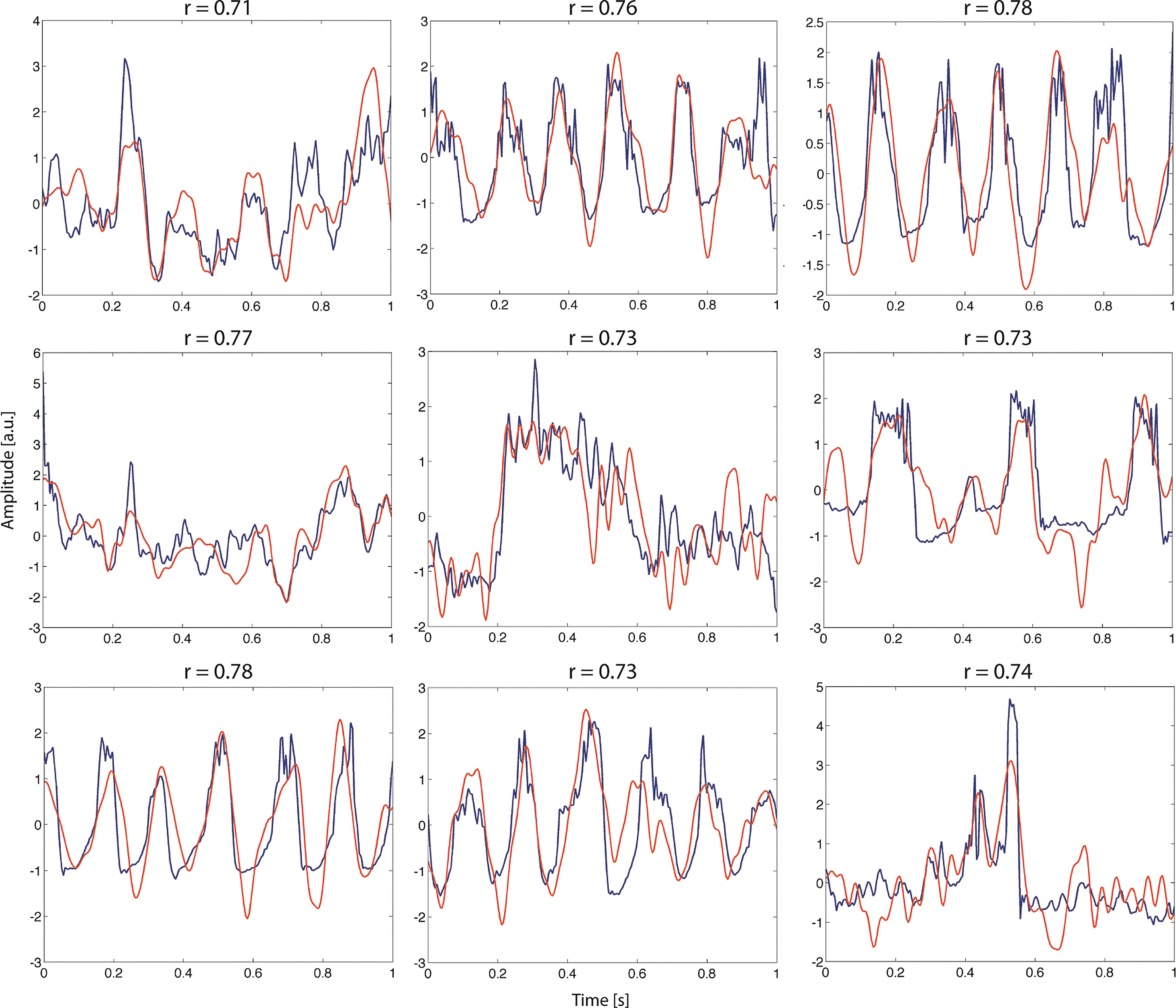
Exemplary motif-fitting results. Shown are one-second snippets of source estimates from EEG (red) and corresponding model fits (blue). Parameters were obtained using a random Monte Carlo search routine that optimized waveform correlation after running for one hour on a single core of a 2.13-GHz Intel Core 2 Duo processor. Despite high correlation coefficients (r=0.78 for the best fit), some waveform features were not captured appropriately. We expect more sophisticated parameter estimation approaches (cf. section A, choice of parameter estimation algorithms) to produce even better fits.
Building a dictionary of dynamical regimes
Automatic parameter optimization heuristics such as evolutionary algorithms are often able to find acceptable solutions in complex optimization problems. However, it is very likely that model parameters that correspond to variable biophysical entities are subject to ongoing variations throughout the course of even short time series, and it hence becomes necessary to refit the parameters for every time segment. Further, a wide range of EEG patterns or time-series motifs are highly conserved and repeatedly appear over the course of an EEG recording (Stern and Engel, 2004). Therefore, it is unreasonable to perform time-consuming searches through the very large parameter space of the coupled network (the number of model instances is 1096 for a parcellation of the brain into 96 regions and 10 free parameters per node) for every short epoch of experimental data. Besides source activity decoupling, we plan to ameliorate this expensive search problem by storing estimation results in a dictionary that associates parameter settings with dynamical regimes.
This dictionary has three major purposes: First, it will help to define priors for subsequent parameter fitting routines and hence reduce computational cost. Second, it is in itself a knowledge database that relates microscopic and mesoscopic biophysical properties—as defined by model parameters—with macroscopic neuronal dynamics. Third, it enables continuous refinement of previous motif candidates. We assume that motifs are highly conserved across subjects, since they resemble instances of prototypic population activity. However, waveform patterns will be subject to small variation, for example, by noise from ongoing background activity. After generating an initially large number of similar good-fitting model waveforms, each waveform is evaluated for its fitness to explain motif patterns across a large number of subjects and signal features. Upon exposure to an increasing number of motif patterns from different subjects and elimination of bad-fitting dictionary entries, only the most generic motif instances will remain in the dictionary. Therefore, only those motif patterns from a class of similarly shaped waveforms that have the highest explanatory power can be seen as most generic and remain in the dictionary.
Such a dictionary maps specific parameter settings to the emerging prototypical model dynamics. Besides waveform, timeseries snippets are classified according to a variety of dynamical features that have relevance for cognition. This may be geometric objects in the state space, that is, flows and manifolds, or a certain succession of relevant signal features, for example, a trajectory of the relative power of frequency bands in each source node or other variables of interest such as RSN patterns, or the presence of prominent features of EEG activity such as sleep spindles, alpha-bursts, or K-complexes. An illustration of the proposed operational flow is shown in Figure 6.
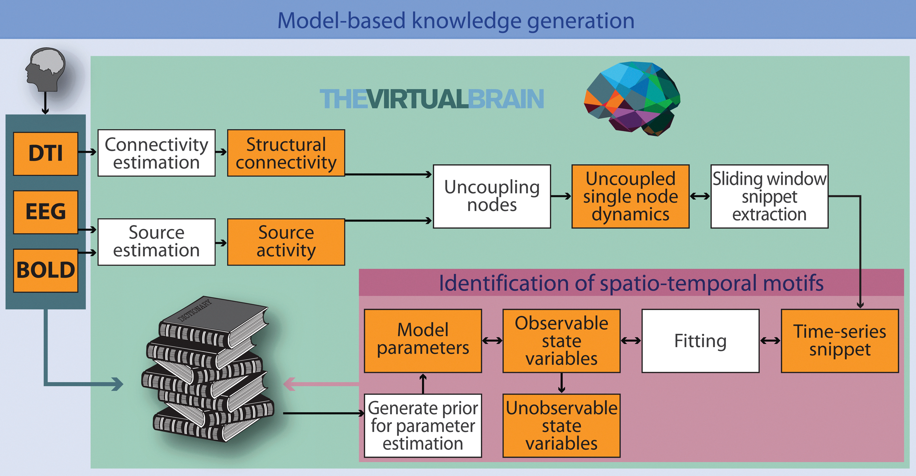
Model-based knowledge generation. The virtual brain estimates parameter sets that enable the model-based replication of short empirical source activity timeseries. Upon emulation of observable timeseries, internal model state variables can then be analyzed to infer knowledge about unobservable system states. Empirical EEG and BOLD data are used to estimate electrical source activity. Employing individual structural priors (fiber-tract capacities and distances), each node's activity can be disentangled from the influences of the other nodes. Spatial and temporal properties of the resulting data are compared to the model output. Parameter settings yielding the best fit are identified. A central point is the identification of spatiotemporal motifs, that is, the identification of similar dynamical behaviors in simulated and empirical data. Matching empirical- and model-based structural flows on manifolds are stored in a dictionary, for example, in the form of prototypical source timecourses. Priors, that is, initial parameter settings known to yield specific classes of dynamics observed in empirical data, are taken from the dictionary for subsequent simulations. Taking advantage from the pool of existing knowledge increasingly reduces the costs for parameter optimization for different empirical dynamical scenarios. In other words, an integrative method of induction and deduction serves our model optimization procedure. Statistical analysis of the parameters sets stored in the dictionary yields the desired insight about which biophysical and/or mathematical settings are related to the different observed brain states.
When fitting new timeseries, instead of re-estimating the parameters for a dynamic regime that might have been inferred before, a dictionary search is conducted, and observed dynamics are related to probable parameter settings. The idea of generating simulation databases was previously successfully applied to several neuroscience models (Calin-Jageman et al., 2007; Doloc-Mihu and Calabrese, 2011; Günay et al., 2008, 2009; Günay and Prinz, 2010; Lytton and Omurtag, 2007; Prinz et al., 2003).
Dictionary-based signal separation was previously successfully applied to several neuroscience problems (Zibulevsky and Pearlmutter, 2001).
To recreate experimental time-series with TVB, we compare variables of interest stored in the dictionary with empirical data. The database can be screened for models that reproduce observed neuronal behavior, and dictionary entries with minimal discrepancy are used as priors for subsequent parameter estimation to keep the search space small; that is, they are used as initial conditions and for the definition of search space boundaries. Further, statistics over the database can give an insight into how specific model configurations relate to the observed neuronal dynamics. To construct the database, the results of previous parameter estimation runs, that is, parameter settings, are stored along with the generated mean-field waveform and metrics of interest that quantify the dynamics of this waveform. Database searches can be based, for example, on waveform correlation or other similarity metrics such as mutual information or spectral coherence, as well as combinations thereof.
Model fitting
The benefits of tuning a model to multimodal empirical data
Simultaneous EEG-fMRI recordings enable us to fit model activity with two different empirical target variables that exist on two different spatiotemporal scales.
On the one hand, the estimated spatiotemporal BOLD activity emerging from fully coupled large-scale model simulations are fitted to match those of empirically measured slow hemodynamic BOLD activity. On the other hand, fast electric dynamics of individual large-scale nodes are fitted to match the corresponding localized source activity derived from EEG source imaging.
Accordingly, we use different metrics to quantify the goodness of fit for the two different spatiotemporal scales. In the case of localized source activity, our target is the reproduction of salient features of the mean-field waveform of source activity. Therefore, we aim to optimize the metrics of interest between empirical and model timeseries such as the least-squares fit between waveforms. Other optimization targets include waveform correlation or coherence and other nonlinear dependence measures such as mutual information. In the case of simulated BOLD signals, we aim for reproducing the global spatial interaction topology. To match spatial FC patterns, the correlation between experimental and simulated FC matrices is maximized.
On the one hand, this enables the forward modeling-based exploration of conditions under which certain FC patterns emerge. On the other hand, we use the fMRI signal to refine ambiguous parameter estimates in situations where it is not possible to determine a unique parameter set that reproduces source activity. This twofold strategy is motivated by the fact that the set of parameters of the full large-scale model can be divided into global and local parameters. While global parameters specify the interaction between distant brain regions, each set of local parameters governs the dynamics of its associated node. To reproduce brain activity by a model, it is necessary to emulate both the uncoupled local dynamics as well as the dynamics emerging from the global interactions between sources. By decoupling the source activity according to the global coupling parameters that were obtained during the forward estimation step, we gain uncoupled source activity. Subsequently, each local node is tuned to reproduce this uncoupled source activity. Note that there is no experimental counterpart of this activity since directly measuring uncoupled intrinsic region activity is impossible as long as brain regions are connected and interacting.
However, if uncoupled local populations are able to reproduce this virtual source activity estimated from empirical data, the full large-scale model will reproduce the originally measured activity after being recoupled again. This uncoupling scheme resembles the straightforward inversion of the coupling scheme implemented in the model. After recoupling sources and performing forward simulations with both estimated parameter sets, the measured EEG-fMRI data are generated on both spatiotemporal scales preserving local source activity that translate to fast EEG activity as well as global source interaction patterns that translate to slow BOLD patterns.
A choice of parameter estimation algorithms
In the following, we review three different parameter estimation approaches we consider most important for accomplishing this task and a method for refinement of solutions based on the integration of the fMRI data. The three approaches are based on stochastic optimization, state observers, and dimensionality reduction. Up to now, only the first approach was used for parameter estimation in the context of TVB, yet we aim to also use the others in the future.
Stochastic optimization
Stochastic optimization (Spall, 2003) is a Monte Carlo parameter estimation strategy that is able to conquer high-dimensional search spaces using random variables. In contrast to a fully randomized search that chooses parameters without any further constraints, during stochastic search, parameters are not generated in an entirely random fashion, but multivariate Gaussian distributions are centered on some initial values, and the algorithm draws a large number of initial parameter sets from this distribution for evaluation. Then, if new points are found to generate better matching results, the multivariate distribution is moved and centered at the new best points in the parameter space. Further, the variance of the distribution is contracted at the end of each iteration, and a smaller part of the search space is searched more thoroughly. Multiple instances of this search engine can be initialized at different starting points and evaluated to increase the chances to find a global minimum and to decrease the probability of getting stuck in the local minima. Examples of how this algorithm is able to fit different motifs found in the source space with the Stefanescu–Jirsa model results are shown in Figure 5.
More sophisticated stochastic methods mimic strategies from biological evolution [Evolutionary computation (Fogel, 2005)], cooling of metals [Simulated annealing (Brooks and Morgan, 1995)], and other biological or physical phenomena [e.g., Ant Colony Optimization, Taboo Search, and particle swarm methods (Dorigo and Di Caro, 1999)].
In the present case, evolutionary approaches are well suited for both parameter sets: the forward model-based estimation of the set of global parameters on longer time-scales and the inverse model-based estimation of local parameters for short time-scales.
Further, the two approaches can be used in a complementary manner to mutually inform themselves about good starting values that correspond to macroscopic phenomena in the case of source space fits or to microscopic phenomena in the case of large-scale fits. For instance, an optimization routine that fits local parameters with snippets that show dynamics on a short time scale can be initialized with parameter values that were obtained during forward simulations that yielded the emergence of RSNs that were observed along with these snippets during the experiment.
Although metaheuristics cannot guarantee to find the global optimum, they often compute the vicinity of global solutions in modest computation times and are therefore the method of choice for large parameter estimation problems (Moles et al., 2003).
State observers
In the framework of control theory, the challenge of parameter estimation in complex dynamical systems is approached by the implementation of state observers aiming to provide estimates of the internal states of a system, given measurements of the input and output of the system. Recently, several state observer techniques have been developed and successfully applied to biological systems, and the use of extended and unscented Kalman filtering methods has become a de facto standard of nonlinear state estimation (Lillacci and Khammash, 2010; Quach et al., 2007; Sun et al., 2008; Wang et al., 2009). When parameters are assumed to be constants, they are considered as additional state variables with a rate of change equal to zero. By incorporating the specific structure of the problem using this state extension, the problem of parameter identification is converted into a problem of state estimation, viz., determining the initial conditions that generate an observed output.
State observers are typically two-step procedures: first, the process state and covariance are estimated from the model. Then, feedback from noisy measurements is used to improve the previous prediction, and the process is repeated until convergence. However, convergence of state estimation is not guaranteed in the nonlinear case if the initial estimates are chosen badly. Even worse, the process of state extension can introduce nonuniqueness of the solution, that is, several sets of parameters or ranges of parameters that produce equally good fits. In this case, the model is referred to as being nonidentifiable.
Dimensionality reduction
A third approach we do consider relevant for generating a dictionary of dynamic motifs, since it corresponds to the state space equivalent of the timeseries motifs: flows on low-dimensional manifolds in a higher dimensional state space.
A data vector of length d can be regarded as a point that is embedded in a d-dimensional space. However, that does not necessarily mean that d is the actual dimension of the data. The intrinsic dimensionality (ID) of a data set equals the minimum number of free variables needed to represent the data without the loss of information. Equivalently, the ID of that data vector is equal to M, if all its elements lie within an M-dimensional subspace. Each extra dimension in regression space considerably hardens parameter estimation (curse of dimensionality); therefore, we seek for a low-dimensional description of our data. Manifolds can be informally described as generalization of surfaces into higher dimensions. Signals and other data can often be naturally described as points and flows on a manifold; that is, they are manifold-valued (Perdikis et al., 2011). Several physiologically motivated models of neuronal activity indicate that neuronal activity patterns have an underlying structure that is inherently lower dimensional and contained on the surface (or tightly around the surface) of a low-dimensional manifold that is embedded within the higher-dimensional data space (Deco et al., 2010; Freyer et al., 2009, 2011, 2012). Therefore, we view manifolds as geometric representations of meaningful system dynamics. To reconstruct manifolds, viz., manifold learning, one seeks for a mapping that projects higher-dimensional input data onto such a low-dimensional embedding while preserving important characteristics of the data. Therefore, describing the system in terms of a dynamic model is equivalent to learning the structure of state space manifolds. The properties of the manifold on which neuronal activity is embedded directly correspond to the intrinsic dynamics of the system. It follows that a model that is intended to capture neuronal dynamics must necessarily reproduce flows on this underlying manifold. Thus, structured flows on manifolds can be regarded as a compact description of the system's dynamics and therefore resemble the state space equivalent of our concept of timeseries motifs.
We outline a three-step procedure for a manifold-based parameter estimation scheme that is based on dimensionality reduction, manifold learning, and subsequent parameter estimation as proposed by Ohlsson and colleagues (2007). The goal of this procedure was to infer a low-dimensional mapping of data points. When data points become constrained to a lower-dimensional manifold, and also regression vectors are, and therefore the dimensionality of the regression problem is equivalently reduced.
Step 1: Dimensionality estimation:
The first step in this process is to estimate the ID of the data. We assume that observed data lie on a limited part of space, and that the dimensionality of this manifold corresponds to the ID of the data, and to the degrees of freedom of the underlying system from which it is generated. It follows that the dimensionality of the data points toward the type and order of a model that can be used for describing the system or to the number of parameters that needs to be estimated if the structure of the model is already known. Consequently, the target dimension for the subsequent manifold learning step, which must be provided for most approaches, is set to the ID of the dataset. Dimensionality estimation (DE) methods can be classified as local or global (Camastra, 2003; Van der Maaten, 2007). Local methods use the information contained in neighborhoods of data points. Specifically, they rest on the observation that the number of data points within a hypersphere around a data point with radius r grows proportionally to rd , with d being the ID of the data. Thus, d can be estimated by counting and comparing the numbers of data points in hyperspheres with different radii. Global DE methods estimate the dimensionality of the full dataset. For instance, principal component analysis (PCA) can be used to estimate the dimensionality of a dataset by defining a cutoff value for the amount of variance that is explained by principal components. Then, the ID of a dataset is equal to the number of principal components that lie above the threshold, since there are typically d components that explain a large amount of variance (where d is the ID of the dataset), whereas the remaining eigenvalues are typically small and only account for noise in the data.
Step 2: Manifold learning:
During this step, one aims to find a transformation of the data into a new coordinate representation on a manifold, termed intrinsic or embedded coordinates, that is, a mapping between the high-dimensional space down to the lower-dimensional space that retains the geometry of the data as far as possible. Many algorithms for manifold learning and dimensionality reduction methods exist and are apart from parameter estimation valuable tools for classification, compression, and visualization of high-dimensional data (Van der Maaten et al., 2009); however, they seldom produce an explicit mapping from the high-dimensional space to intrinsic coordinates. Instead, the algorithm has to be rerun as new data are introduced. However, Ohlsson and his colleagues (2007) propose a remedy for this problem by linearly interpolating between implicit mappings. In the remainder of this section, we will list some approaches to exemplify some general ideas manifold learning techniques are based on and leave it to the reader to pick a suitable method for the specific properties of their data from the referenced literature. For dimensionality reduction algorithms, one commonly distinguishes between linear techniques, including traditional methods such as PCA and linear discriminant analysis (LDA), and nonlinear techniques as well as between the global and local techniques. The purpose of the global techniques is to retain global properties of the data, while local techniques typically only maintain properties of small neighborhoods of the data. Similar to PCA and LDA, global nonlinear techniques preserve global properties of the data, but are, in contrast, able to generate a nonlinear transformation between the high- and low-dimensional data. Multidimensional scaling (MDS) (Cox and Cox, 2000) seeks a low-dimensional representation that preserves pairwise distances between data points as much as possible by minimizing a stress function that measures the error between the pairwise distances in the low-dimensional and the high-dimensional representation. Stochastic proximity embedding (Agrafiotis, 2003) also aims at minimizing the multidimensional scaling raw stress function, but differs in the efficient rule that it employs to update the current estimate of the low-dimensional data representation. Isomap (Tenenbaum, 1998) overcomes a weakness of MDS, which is based on Euclidean distances, by accounting for the distribution of neighboring data points using geodesic distances. If the high-dimensional points lie on a curved surface, Euclidean distance underestimates their displacement, while geodesic (or curvilinear) distance measures their actual stretch over the manifold. Maximum variance unfolding (Weinberger et al., 2004) aims at unfolding data manifolds by maximizing the Euclidean distance between data points while keeping the local geometry, that is, all pairwise distances in a neighborhood around each point, fixed. Diffusion maps (Lafon and Lee, 2006) are constructed by performing random walks on the graph of the data. Therefore, a measure of the distance of data points is obtained, since walking to a nearby point is more likely than walking to one that is far away. Using this measure, diffusion distances are computed with the aim to retain them in the low-dimensional representation. Kernel PCA is an extension of PCA incorporating the kernel trick (Schölkopf et al., 1998). In contrast to traditional linear PCA, Kernel PCA computes the principal eigenvectors of a kernel matrix, instead of those of the covariance matrix. The kernel matrix is computed by applying a kernel function to data points that map them into the higher-dimensional kernel space, yielding a nonlinear mapping. Generalized discriminant analysis (Baudat and Anouar, 2000) is the kernel-based reformulation of LDA that attempts to maximize the Fisher criterion (similar to LDA) in the higher-dimensional kernel space. Multilayer autoencoders (Hinton and Salakhutdinov, 2006) are feed-forward networks with an odd number of hidden layers that are trained to minimize the mean-squared error between the input and output, which are ideally equal. Consequently, upon minimization, the middle layer constitutes a coded, low-dimensional representation of the data. Local nonlinear techniques include local linear embedding (LLE), Laplacian eigenmaps, Hessian LLE, and local tangent space analysis (LTSA). LLE (Roweis and Saul, 2000) assumes local linearity, since it represents a data point as a linear combination of its nearest neighbors by fitting a hyperplane through these points. During Hessian LLE (Donoho and Grimes, 2003), the curviness of the high-dimensional manifold is additionally minimized when embedding it into a low-dimensional space. Similarly, LTSA (Zhang and Zha, 2004) represents high-dimensional data points by linearly mapping them to the local tangent space of a data point. Thereby, it provides the coordinates of the low-dimensional data representations, along with a linear mapping of those coordinates to the local tangent space of the high-dimensional data. The Laplacian eigenmaps technique (Belkin and Niyogi, 2001) preserves pairwise distances between neighboring points by finding a representation that minimizes the distances between a data point and its k nearest neighbors. Apart from strictly global or local methods and extensions and variants thereof [cf. Van der Maaten et al. (2009) for further reading], there also exist hybrid techniques that combine both types of methods by computing several linear local models along with a global alignment of these local embeddings, for example, locally linear coordination (Teh and Roweis, 2002), manifold charting (Brand, 2003), and coordinated factor analysis (Verbeek, 2006).
Step 3: Manifold-based gray box identification:
Manifold-based regression (Ohlsson, 2008) can be combined with prior physical knowledge about the dynamics of the data in the form of a dynamical model. Ohlsson and Ljung (2009) recently developed a technique for manifold-based gray box system identification that they dub weight determination by manifold regularization. They propose a new regression algorithm that enables the inclusion of prior knowledge in high-dimensional regression problems, that is, gray-box system identification. The physical knowledge expressed by a dynamical model is introduced into the regression problem by addition of a regularization term to the optimization function that results in high cost, if the regressors expressed in the coordination of the manifold do not behave according to the physical model. The manifold generating optimization problem then also minimizes over the states of the state space model and hence tries to find a coordination of the manifold that can be well described by the assumed model and at the same time fit well with the manifold assumption and the measured output. Apart from this specific implementation, a manifold-based approach offers exciting possibilities for the integration of empirical data with physical models as well as visualization and analysis of dynamical properties of the system under study that should be extended in the future.
Identifiability: capitalizing on multimodal empirical data
When the number of unknown parameters is very large, parameter estimation schemes often find several equally fitting parameter sets, or ranges of values, instead of a unique optimal solution. In these cases, the model is qualified as nonidentifiable. Due to the large extend of the parameter space of the full model, the solution of parameter estimation will be characterized by large uncertainties and nonuniqueness with a high probability of existence of infinite sets of parameters that are equally likely to be correct. Given one or several sets of model parameters that generate equally good estimates, one may ask, what is the probability that model parameters are correct? The parameters of the underlying natural system, that is, the biophysical properties that relate to our model parameters, only have a single realization at a particular time.
In a model situation, the likelihood of a parameter set is the probability that an observed data set is generated given this parameter set. However, the computation of likelihoods is very costly when the dimensionality of the data is high. As a remedy, it is possible to include additional information about the system under study that was not used for fitting. To improve the probability of finding the correct solution, we introduce additional criteria that discern plausible from implausible estimates. In our case, we plan to obtain this additional information from an fMRI signal that was simultaneously acquired with the EEG.
In the context of biological systems, this problem has been addressed by an approach that combines extended Kalman filtering with a posteriori calculated measures of accuracy of the estimation process based on a χ2 variance test on measurement noise (Lillacci and Khammash, 2010). The core idea is to examine the reliability of estimates after they have been computed by using additional information gathered from noise statistics from the experiment to ensure that the estimated parameters are consistent with all available empirical data or otherwise defined constraints. After each estimation step, the algorithm checks whether the estimate satisfies several constraints. This step can be cast as a separate optimization problem. If the estimate fullfills the constraints, the algorithm was able to recover the unique solution to the problem and continues with this estimate. If not, most likely, no unique solution exists, and the estimate is replaced by the solution of the constraint satisfaction problem, and the parameter search continues on the basis of the thereby yielded refined estimate.
Following these lines, we propose an additional a posteriori test for refinement of candidate parameter sets that were obtained during the estimation steps using one of the above-listed parameter estimation approaches. In our case, we exploit the existence of two simultaneously acquired data sets that capture partially complementary dynamics on two different time scales. While fitting the model to the fast dynamics, we use the slow BOLD dynamics for verifying the previous estimates and selecting among ambigious estimates. The time resolution of fMRI observations is much lower than that of EEG observations, with typically one datapoint every 2 sec. In principle, this setup could be modeled by directly fusing both signals using a time-varying observation matrix integrating EEG and fMRI into a single-observation model (Purdon et al., 2010). Moreover, it would also be possible to directly integrate BOLD-derived inequality constraints by using constrained Kalman filtering approaches (Simon and Chia, 2002; Simon and Simon, 2003) or to extend approaches for the slow–fast systems. However, BOLD observations do not need to be integrated directly in the observation model, but can be used it in the line of Lillacci and Khammash (2010) for selection between ambiguous estimates.
What is the additional information that we can extract from BOLD data that allow a further refinement of initial estimates? It is well recognized that EEG mainly reflects the superpositioned and spatiotemporally smoothed version of electrical activity of pyramidal neurons in the superficial layers of the cortex oriented that are oriented perpendicular to the scalp (Buzsáki et al., 2012). Since we fitted the model with the source-projected EEG data, it is reasonable to assume that only the activity of excitatory neurons is captured. However, there is evidence estimating that the activity of inhibitory neurons, which comprise about 15%–20% of cortical neurons, accounts for 10%–15% of the total oxidative metabolism (Attwell and Iadecola, 2002). In contrast to pyramidal cells, internerons that majorily represent the inhibitory cell fraction do not have a dipolar configuration and hence do not contribute to the EEG signal—while they are suppoed to have a metabolic demand. Despite there is ongoing debate whether and how inhibitory activity influences the BOLD signal (Ritter et al., 2002), consensus exists that fMRI sees a fraction of neuronal activity that—although indirectly—EEG is not able to detect. Therefore, it becomes possible to use the additional information that is unobservable with EEG to refine previous fits of the model with EEG data. A simple example of several candidate parameter sets that produce equally fitting, similarly shaped electric waveforms have been identified. Thereby, mean-field timeseries of the inhibitory population have been generated by the model. This additional information can then be incorporated into forward BOLD data simulation, and the resulting BOLD waveform and FC topology can be used as an additional crtierion for discerning between parameter candidates.
Another refinement strategy is based on the robustness of a parameter set to explain (1) increasingly longer snippets and (2) more snippets across different subjects. We assume that the motif patterns constitute distinct activity profiles of neural population dynamics that appear highly conserved in different subjects, but exhibit slight variations due to background activity. Therefore, the quality of a parameter set can be quantified by its robustness in explaining a noisy motif pattern across a large number of different subjects. Thus, it is possible to assign the scores to parameter sets that rank their robustness in predicting motif patterns across different subjects. Equally fitting parameter sets can be initially stored in the dictionary and subsequently dismissed, as the model is fitted to longer snippets and to new data sets from different subjects.
Despite the existence of Kalman filter approaches for filtering systems with multiple timescales, that is, slow–fast systems, and further, approaches that directly incorporate inequality constraints, we prefer the proposed two-step estimation–refinement procedure out of several reasons. First, it constitutes a convenient way to add further constraints that are unknown at the time of the estimation, but becomes available later a posteriori. Therefore, we store all parameter settings that allow the reproduction of a certain waveform in a dictionary and apply pruning of the results upon availability of new physiological constraints. Second, besides the fact that an additional BOLD model increases the already-huge space of unknowns that need to be fitted and thereby hardening the estimation process, we are uncertain about the actual neurovascular coupling, and this uncertainty might bias the estimator and introduce more disadvantages than benefits when fitting the model to data. Facing the lack of knowledge about the exact inter-relationship between neuronal activity and hemodynamic signal changes, our agenda is to use the least amount of assumptions about electrovascular coupling as possible and to stay as flexible as possible to use this information only for refinement of fittings of electrical activity. Third, the forward BOLD model might change. Since we use a very simple BOLD model at the present time and it is very likely that better spatiotemporal BOLD models will appear in the near future, we want to keep the flexibility to incorporate new models without the necessity to repeat the estimation runs. Fourth, we are actually interested in ambiguous solutions, since parameter settings that allow the emergence of certain dynamics directly correspond to physiological ranges and conditions under which a certain behavior is possible in the real system. This allows an in silico study of physiological properties of the neural populations that permit the emergence of certain activity patterns. This in turn enables us to formulate hypotheses that can be verified in vitro or in vivo later on.
Benefits of TVB Platform
Predicting unobservable internal states and parameters: model-based formulation of new hypotheses
By identifying parameter trajectories, we also identify phase flows of unobservable system components; that is, we build a computational microscope that allows the inference of internal states and processes of the system that lie below the resolution of the imaging device. For example, it is impossible to observe the neuronal source activity of the entire human brain simultaneously. If at all, we have patients with implanted single electrodes or grids capturing a certain region, so that only local field potentials or multiunit activity can be assessed at one time. With our modeling approach, we are able to predict the electric source activity that underlies our observed EEG and fMRI signals throughout the brain simultaneously. An example of source activity in 96 regions of the brain is shown in Figure 3A (right).
In a similar vein-fitting model, parameters to empirical data lead to the prediction of certain biophysical properties of the system units, given the observed functional imaging data. For example, altering the coupling factors K11, K12, and K21 between the inhibitory and excitatory neuronal population of the mesoscopic node modifies the properties of the resulting source activity. This leads to the quantitative hypotheses of the role of the balance between inhibitory and excitatory local coupling testable by means of a pharmacological intervention using selective gamma-aminobutyric acid or glutamate antagonists/agonists.
Another issue addressable by TVB is the relation between electric neuronal activity and the BOLD signal. This is so important since fMRI is such a widely used brain-imaging tool. However, the link between the BOLD signal and electrophysiological signals is far from being clear. In particular, the link between fast oscillatory activity—a dominant feature of electrophysiological data—and the BOLD signal is not resolved (Riera and Sumiyoshi, 2010). While the strengths of those oscillations that are thought to reflect the degree of synchrony in the underlying neuronal populations is correlated with the BOLD signal (Moosmann et al., 2003; Ritter et al., 2008, 2009), the biophysical principles of this coupling are still unrevealed. Yet, gaining more insight about this relation is essential, since evidence attributes important functional roles to neuronal oscillations and synchrony. Changes of these variables are indicators for functionally relevant brain state alterations (Becker et al., 2011; Freyer et al.; Reinacher et al., 2009). TVB offers the possibility to explore both the interrelations of different types of neuronal activity and the neurohemodynamic coupling. The former is relevant to examine the neuronal mechanisms underlying brain function such as the highly debated question whether phase resetting of ongoing oscillations is a common principle in the brain (Ritter and Becker, 2009). The latter is relevant to clarify how oscillations, their phase, and synchrony behavior relate to the BOLD signal. The dictionary approach allows us to identify and store parameter sets that yield best model fits to multimodal empirical data. Such information can be collected for large numbers of data sets. Post hoc statistics over the collected parameter sets and corresponding goodness of fits allow us to identify mechanistic scenarios that yield with high reliability our empirical observations. The unobservable states predicted by such identified models can then be used to formulate new hypotheses, for example, about underlying molecular mechanisms that can be tested by means of appropriate methods such as intracranial recordings, pharmacological interventions, or in vitro research.
Revealing mechanisms that yield specific features of large-scale dynamics
EEG waveforms recorded on the scalp are a linear superposition of microcurrent sources. However, the mechanisms of source interaction from which dynamic signals emerge remain mostly unknown. In the past, it has been shown that time delays of signal transmission between large-scale brain regions that emerge from the specific underlying large-scale connectivity structure due to finite transmission speeds can have a profound impact on the dynamic properties of the system (Ghosh et al., 2008; Knock et al., 2009). Ghosh and colleagues demonstrate that in large-scale models, besides realistic long-range connectivity, the addition of noise and time delays enables the emergence of fast neuroelectric rhythms in the 1–100-Hz range and slow hemodynamic oscillations in the ultraslow regimes <0.1 Hz (Ghosh et al., 2008). These two studies demonstrate how large-scale modeling helps to reveal mechanisms that based on empirical data alone would not have been recovered. The same large-scale modeling approaches that have been employed in both studies now build important foundations of TVB.
TVB accounts for individual differences in SC. Hence, it can be used to investigate the effects of variation in coupling (time delays and connection strengths) on emerging brain dynamics by comparing predictions and real data across different subjects. Figure 2C illustrates how TVB can reveal individual structure–function relations. SC in terms of fiber-tract sizes and length was determined for a single subject (No. 7). A Stefanescu–Jirsa full-brain model was constructed based on the features of the SC of this subject. Simulations were run for 80 different parameter settings. The resulting 96×96 simulated BOLD FC matrices were compared with the empirical BOLD FC matrices of this subject and of eight others. The distribution of correlation coefficients between the simulated (based on the connectivity of subject No. 7) and the empirical (of all nine subjects) FC for a single tested parameter setting (Table 2) is displayed in Figure 2C. Each subplot represents the distribution of correlation coefficients obtained for the empirical FCs of an individual subject. In this example, model predictions match far better the empirical data of subject No. 7, that is, the subject whose SC was used. A systematic evaluation of these results will be published elsewhere. This example illustrates that TVB enables us to assess the individual structure–function relationship of the brain. Statistical evaluations over a larger number of subjects will provide us with insights regarding which structural parameters give rise to which features of the space–time structure of brain activity, and hence helps us understanding interindividual differences.
DTI, diffusion tensor imaging.
The role of several features concerning the relation between structure and dynamics as well as the relation between source activity and the signals observed with brain imaging devices can be addressed by TVB. To mention just a few, the role of time delays, directionality of information flow, or synchrony in certain frequency bands or between regions can be systematically investigated by TVB. As an illustration we show in Figure 7, how different frequency bands of electric source activity do reflect the functional BOLD connectivity observed in empirical data.
Following the reconstruction of model dynamics from empirical timeseries, several neurobiological questions can be addressed. State and parameter space trajectories can be related to experimental conditions and behavior. Therefore, the proposed approach allows for the direct association of low-level neuronal processes with the top-level cognitive processes. It identifies metrics that quantify the functional relevance of dynamical features for cognition and behavior under normal and pathological conditions. Ultimately, we believe that this tool enables us to gain further insights into the mechanisms and principles of neural computation.
Conclusions
In this article, we have shown the development of a computational platform called TVB that aims to model large-scale brain dynamics as accessible by brain-imaging methods such as EEG and fMRI. We chose the Stefanescu–Jirsa model for the simulation of local dynamics at 96 cortical regions. These regions or nodes were connected to form a network. Time delays and interaction strength between the nodes were based on real tractography data of individual subjects.
This is the first open-source computational platform that provides a complete and customizable toolbox to model large-scale brain phenomena of individual subjects. It enables identification of mechanisms underlying the space–time structure of the brain and the generation of new hypotheses not possible experimentally. Thereby, it integrates theory-driven and data-driven research approaches into a single framework.
While we have provided here a proof of concept for the functioning of TVB, TVB is a community project. Only the contributions of many sites will lead to a major breakthrough in our understanding of the brain. It is the systematic and standardized exploration of model dynamics on multiple spatiotemporal scales and the organized storage of new knowledge in the TVB dictionary that finally will give us an understanding of the principles that underlie the complex space–time structure of our brain.
Footnotes
Acknowledgments
The authors acknowledge the support of the James S. McDonnell Foundation (Brain Network Recovery Group JSMF22002082) granted to P.R., A.R.M., and V.J.; the German Ministry of Education and Research (Bernstein Focus State Dependencies of Learning 01GQ0971) granted to P.R.; and the Max-Planck Society (Minerva Program) granted to P.R.
Author Disclosure Statement
No competing financial interests exist.