Sage Journals: Discover world-class research

Abstract

We introduce a method called neighbor-based bootstrapping (NB2) that can be used to quantify the geospatial variation of a variable. We applied this method to an analysis of the incidence rates of disease from electronic medical record data (International Classification of Diseases, Ninth Revision codes) for ∼100 million individuals in the United States over a period of 8 years. We considered the incidence rate of disease in each county and its geospatially contiguous neighbors and rank ordered diseases in terms of their degree of geospatial variation as quantified by the NB2 method. We show that this method yields results in good agreement with established methods for detecting spatial autocorrelation (Moran's I method and kriging). Moreover, the NB2 method can be tuned to identify both large area and small area geospatial variations. This method also applies more generally in any parameter space that can be partitioned to consist of regions and their neighbors.

Introduction

As the number of sources and the volume of electronic medical records (EMR) and electronic health records increases, there is a growing ability to aggregate these data and extract information about population and public health.^1,2 Over the past several years, new sources of digital health data, such as web searchers, social media, mobile phones, and personal health sensors have increased the number of sources and data volumes even more.^3–5 Much of these data can be geocoded with location information so that techniques from spatial epidemiology can be used to explore geospatial variation in disease, health outcomes, and population health using disease mapping, disease cluster analysis, and related techniques.^6–9 With this much geocoded digital health data, there is a need for simple tools and algorithms that can be used by researchers across disciplines for identifying the presence of spatial autocorrelation in disease incidence data, especially in large datasets.¹⁰

An initial starting point for evaluating the presence of patterns in disease or other geocoded data is determining whether the data are spatially autocorrelated, that is, whether the disease rates or values of interest are similar in nearby areas and fall off with distance, which could indicate the presence of core areas of disease risk.^11,12

We introduce a Monte Carlo based algorithm that we call neighbor-based bootstrapping (NB2) that can be used to quantify geospatial autocorrelation. We apply this algorithm to ∼100 million geocoded EMR and rank order 548 diseases as determined by International Classification of Diseases, Ninth Revision (ICD-9) codes from those with the strongest geospatial autocorrelation to those with the weakest geospatial autocorrelation. We compare this method's results to Moran's I statistic¹³ and to kriging,^14(p.44) two other techniques that have been used to quantify geospatial autocorrelation. The spatial size scale of disease patterns may range widely from small, localized affected regions to larger affected areas, depending on the nature of the underlying factors. We have developed two versions of the NB2 ranking, one favoring patterns of tight clusters and the other favoring broader less peaked patterns. In the Supplementary Data section, we provide the results of these two versions on NB2 ranking by category of disease and detail the spatial patterning of highly ranked ICD-9 codes (Supplementary Data are available online at www.liebertpub.com/big).

Applying geospatial analysis and visualization techniques to geocoded health data has long been understood to be important for identifying risk factors from the physical environment and for providing insights into the transmission of infectious and vector-borne diseases.^15–21 For example, spatial analysis of health data can be used to identify and manage risk associated with proximity to potentially harmful environmental exposures, such as chemical toxins or air pollutants.^18,22,23 More generally these techniques are also important for understanding a broader range of risk factors, including risk factors from the demographic, economic, social, cultural, regulatory, or legal environments.^24–32

Materials and Methods

Data

The dataset consists of EMR data from the Truven Health MarketScan Commercial Claims and Encounters Database, which includes approved inpatient and outpatient insurance claim information for a total of ∼100 million unique and de-identified individuals across the United States for the time period from 2003 to 2010. The records include 1.3 billion diagnostic ICD-9 subdivided codes (12.89 unique codes per person), geotagged by county Federal Information Processing Standards code. Here, we restrict to using the ∼800 non-subdivided ICD-9 codes from 001 to 799, which excludes injuries, poisonings, and accidents. We refer to ICD-9 codes by the three digit integer group. (e.g., “005: Other bacterial poisoning” includes “005.0 Staphylococcal food poisoning.”)

We also restrict our analysis to the 3109 counties in the continental United States and to the ICD-9 codes that have data for two-thirds or more of the counties. This leaves 548 ICD-9 codes.

For each of these 548 codes, we adjust for age and gender by using standard populations³³ as follows. We determine crude incidence rates for the standard 19 groups of age populations for each gender by taking raw counts for each group and dividing by the population at risk, which in this case we take to be the total number of records for each county for each age/gender group converted to 100,000 person-year units: \documentclass{aastex}\usepackage{amsbsy}\usepackage{amsfonts}\usepackage{amssymb}\usepackage{bm}\usepackage{mathrsfs}\usepackage{pifont}\usepackage{stmaryrd}\usepackage{textcomp}\usepackage{portland, xspace}\usepackage{amsmath, amsxtra}\usepackage{upgreek}\pagestyle{empty}\DeclareMathSizes{10}{9}{7}{6}\begin{document} \begin{align*} Y_ { crude } ^ { age , gender } = { \frac { { \kern 1pt } { \rm { cases } } \; { \rm { of } } \; { \rm { ICD-9 } } { \kern 1pt } } { { \kern 1pt } { \rm { total } } { \rm { cases } } { \kern 1pt } } } \times { \frac { 100000 { \kern 1pt } { \rm { persons } } { \kern 1pt } } { 8 { \kern 1pt } { \rm { years } } { \kern 1pt } } } . \tag { 1 } \end{align*} \end{document}

In Equation (1), for each of the 548 truncated ICD-9 codes, by cases of ICD-9, we mean the count of the number of occurrences in the data of that ICD-9 code with the specified age and gender.

The age and gender adjusted rate is calculated by multiplying the crude rate for each group by the appropriate weight using the Census 2010 standard population and summing the products³⁴: \documentclass{aastex}\usepackage{amsbsy}\usepackage{amsfonts}\usepackage{amssymb}\usepackage{bm}\usepackage{mathrsfs}\usepackage{pifont}\usepackage{stmaryrd}\usepackage{textcomp}\usepackage{portland, xspace}\usepackage{amsmath, amsxtra}\usepackage{upgreek}\pagestyle{empty}\DeclareMathSizes{10}{9}{7}{6}\begin{document} \begin{align*} { Y_ { adjusted } } = { \Sigma _ { age , gender } } Y_ { crude } ^ { age , gender } \times { \frac { { \kern 1pt } { \rm { group } } \; { \rm { population } } { \kern 1pt } } { { \kern 1pt } { \rm { total } } \; { \rm { population } } { \kern 1pt } } } \tag { 2 } \end{align*} \end{document}

NB2 method

The NB2 method uses resampling to evaluate in this example whether or not the incidence rate of a disease can be accurately estimated from the incidence rate of the disease in counties that are neighbors. The first step in this method is to define regions and neighbors of regions. Here we define regions as counties and neighboring counties as counties that are geospatially contiguous to the county's polygon border, including vertices (Queen style), though it is important to note that there are many options to consider when defining neighbor relationships (contiguity, distance, spatial weights) that have varying effects on results.^35,36 In this article, we focus on geospatially defined neighbors, but an advantage of this method is that it is applicable without change to neighbors in any space of features, not just neighbors in two or three-dimensional physical space.

We compute a bootstrapped estimate as follows. Fix a county Y. For each ICD-9 code, we sample with replacement a set of neighboring counties and a set of random counties and compare the normalized disease incidence [from Eq. (2)].

More explicitly, fix a county Y and assume that it has n^Y neighbors. We estimate the log incidence rate Z_neighbor for county Y as the average log incidence rate of a list of n^Y randomly chosen (with replacement) neighboring counties. We also estimate for each county the log incidence rate Z_random for county Y as the average log incidence rate of n^Y randomly chosen (with replacement) counties from the full set of all counties. These counties may or may not be neighbors.

We compare the two estimates (neighbors vs. random) to the known log incidence for each of the drawn counties in two separate ways (see Algorithms 1 and 2).

In the first implementation, we take the difference from actual of the estimates of Z_neighbor versus Z_random. We then use a paired Student's t-test to evaluate whether neighbor-based predictions are a significant improvement over random prediction. For ICD-9 codes with significant underlying spatial patterns, we expect that the Z_neighbor estimates will be significantly closer to actual than the Z_random estimates.

We repeat this process to obtain 1000 estimates of the neighbor-based versus random differences, and for each of these compute the paired t-test. We then take the median t-test value from these 1000 estimates. This gives us one t-test statistic value per ICD-9 code, describing how closely related incidence rates of that ICD-9 are in neighboring counties as compared with a random selection of counties.

In the second implementation, we compare the neighbors versus random estimates by counting, for each pair of bootstraps, the number of samples where the neighbor estimate is closer to actual than the random estimate. We then repeat this 1000 times, take the median number, and using this to calculate the log odds that the neighbor estimate is more accurate than the random estimate.

Algorithm 1:

Neighbor-based bootstrapping method with paired t-test

INPUT: Set of records, {counties} with length N; the value of interest (log incidence rate Z) for each record Y; and the list of each record's neighbors {neighbors(Y)}.

OUTPUT: N B2 statistic using paired t-test

for m ← 1 to M repetitions do

for N samples (with replacement) of Y ∈ {counties} do

Z^Y ← log (incidence rate in county Y)

n^Y ← number of elements in {neighbors(Y)}

Choose n^Y counties ∈ {neighbors(Y)} with replacement, call this B_neighbor

Choose n^Y counties ∈ {counties} with replacement, call this B_random

average Z of B_neighbor

average Z of B_random

end for

D_neighbor ← List of

₋ Z^Y for N sampled counties

D_random ← List of

₋ Z^Y for N sampled counties

Set t^m equal to the paired Student's t-test statistic for D_neighbor and D_random:

\documentclass{aastex}\usepackage{amsbsy}\usepackage{amsfonts}\usepackage{amssymb}\usepackage{bm}\usepackage{mathrsfs}\usepackage{pifont}\usepackage{stmaryrd}\usepackage{textcomp}\usepackage{portland, xspace}\usepackage{amsmath, amsxtra}\usepackage{upgreek}\pagestyle{empty}\DeclareMathSizes{10}{9}{7}{6}\begin{document} $$ { t^m } = ( { \bar D_ { neighbor } } - { \bar D_ { random } } ) \sqrt { { \frac { l ( l - 1 ) } { \sum \nolimits_ { i = 1 } ^l \left( \hat D_ { neighbor } ^l - \hat D_ { random } ^l \right) } } } $$ \end{document}

end for

t ← List of t^m for all M repetitions

NB2 statistic = median(t)

Algorithm 2:

Neighbor-based bootstrapping method with log odds

INPUT: Set of records, {counties} with length N; the value of interest (log incidence rate Z) for each record Y; and the list of each record's neighbors {neighbors(Y)}.

OUTPUT: N B2 statistic using log odds

for m ← 1 to M repetitions do

for N samples (with replacement) of Y ∈ {counties} do

Z^Y ← log (incidence rate in county Y)

n^Y ← number of elements in {neighbors (Y)}

Choose n^Y counties ∈ {neighbors(Y)} with replacement, call this B_neighbor

Choose n^Y counties ∈ {counties} with replacement, call this B_random

average Z of B_neighbor

average Z of B_random

end for

Z_neighbor ← List of

for N sampled counties

Z_random ← List of

for N sampled counties

Set u^m equal to the number of samples where the neighbor estimate is closer to actual than the random estimate:

u^m = length(abs(Z_neighbor − Y) < abs(Z_random − Y) = = TRUE))

end for

u ← List of u^m for all M repetitions

NB2 statistic

\documentclass{aastex}\usepackage{amsbsy}\usepackage{amsfonts}\usepackage{amssymb}\usepackage{bm}\usepackage{mathrsfs}\usepackage{pifont}\usepackage{stmaryrd}\usepackage{textcomp}\usepackage{portland, xspace}\usepackage{amsmath, amsxtra}\usepackage{upgreek}\pagestyle{empty}\DeclareMathSizes{10}{9}{7}{6}\begin{document} $$= \log \left( { { \frac { median ( u ) } { N - median ( u ) } } } \right)$$ \end{document}

Results

Performance

We first evaluated the impact of varying the number of times M that we resampled. Running the entire procedure and resampling M = 1000 times for all 548 diseases takes just over 28 hours on a virtual machine with 8 Xeon cores running at 2.00 GHz with 16 GB of RAM. This is about 25 minutes per disease using a single core.

For 100 bootstraps, the run time for 548 diseases on 8 cores takes about 220 minutes, or a little over 3 minutes per disease when using a single core. Comparing the NB2 statistic values for 1000 versus 100 simulations, the difference on average is 0.2% and at maximum 1.9%. For 10 bootstraps, the total run time is about 30 minutes, or about 30 seconds per disease using a single core. The mean difference between NB2 statistic values for 1000 and 10 simulations is 0.2%, and the maximum difference is 5.1%. The results are summarized in the table below.

No. of bootstraps (M)	Time (minutes)	Mean difference	Max. difference	Standard deviation difference
1000	25	NA	NA	NA
100	3	0.2%	1.9%	0.4%
10	0.5	0.2%	5.1%	0.9%

In the analysis that follows, we are primarily focused on the rank ordering of the ICD-9 codes according to these two implementations of the NB2 method. There is no significant difference in the rank orderings between 1000 and 100 or 10 repeated bootstraps.

Comparison with Moran's I statistic

We compare the neighbor-based bootstrapping results to the global Moran's I statistic for detecting spatial autocorrelation, which is based on the sum over weights between units multiplied by the mean-adjusted outcome of interest divided by the squared mean difference of each point. Moran's I is defined as¹³: \documentclass{aastex}\usepackage{amsbsy}\usepackage{amsfonts}\usepackage{amssymb}\usepackage{bm}\usepackage{mathrsfs}\usepackage{pifont}\usepackage{stmaryrd}\usepackage{textcomp}\usepackage{portland, xspace}\usepackage{amsmath, amsxtra}\usepackage{upgreek}\pagestyle{empty}\DeclareMathSizes{10}{9}{7}{6}\begin{document} \begin{align*} I = \frac { n } { { { \Sigma _i } { \Sigma _j } { w_ { ij } } } } { \frac { { \Sigma _i } { \Sigma _j } { w_ { ij } } ( { y_i } - \bar y ) ( { y_j } - \bar y ) } { { \Sigma _i } { { ( { y_i } - \bar y ) } ^2 } } } \tag { 3 } \end{align*} \end{document}

where n is the total number of spatial polygons (counties), y_i is the value of interest of the ith polygon, \documentclass{aastex}\usepackage{amsbsy}\usepackage{amsfonts}\usepackage{amssymb}\usepackage{bm}\usepackage{mathrsfs}\usepackage{pifont}\usepackage{stmaryrd}\usepackage{textcomp}\usepackage{portland, xspace}\usepackage{amsmath, amsxtra}\usepackage{upgreek}\pagestyle{empty}\DeclareMathSizes{10}{9}{7}{6}\begin{document} $$\bar y$$ \end{document} is the global mean, and w_ij is the spatial weight of the link between polygon i and j.

Moran's I ranges from −1 (perfect dispersion, as in a black and white checkerboard pattern) to 1 (black squares on one side, white on the other). A random distribution would have I close to 0. We compare the values of Moran's I for the set of log incidence rates across counties for each ICD-9 code to both the implementation of the NB2 method using the paired Student's t-test evaluation and the implementation using the log odds evaluation. If the geospatial variation that the NB2 method detects is similar to Moran's I, then the NB2 statistic values should increase as Moran's I goes to 1. In Figure 1, we show the NB2 t-test statistic estimate (left) and the log odds estimate (right) plotted against Moran's I statistic for all ICD-9 codes tested. In this figure, on both the left and the right, there is a data point for each of the ICD-9 codes tested. Generally, the NB2 statistic values increase as Moran's I statistic increases, though there is noticeable scatter.

FIG. 1.

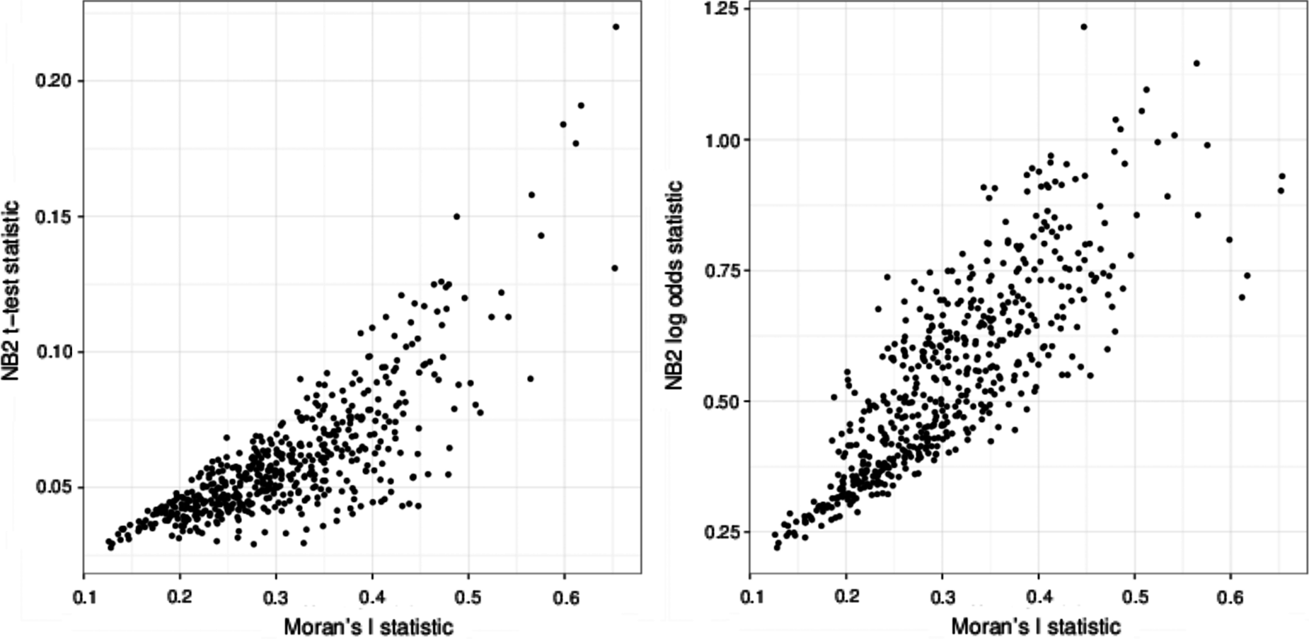
Comparison of this NB2 method with Moran's I statistic for detecting spatial autocorrelation. We show the NB2 experiment's ability to detect spatial correlation (y-axis) measured by the paired Student's t-test estimate (left) and the log odds estimate (right) for the neighbor county predictions versus random county predictions plotted against the Moran's I statistic estimate (x-axis). NB2, neighbor-based bootstrapping.

We rank ordered the ICD-9 codes using the two NB2 method implementations and the Moran's I statistic to produce three ordered lists of ICD-9 codes from the strongest spatial correlation (largest Moran's I statistic, largest NB2 t-test, largest NB2 log odds test) to the weakest. Tables 1 –3 contain the top 25 ICD-9 codes for both NB2 implementations and Moran's I. Here, we will compare the properties of the spatial distributions for ICD-9 codes ranked highly by the two NB2 procedures with those ranked highly by Moran's I statistic.

Table 1.

Top 25 ICD-9 codes as ranked by neighbor-based bootstrapping (t-test)

NB2 (t-test)	NB2 (odds)	Moran	ICD-9 diagnosis name	ICD-9	Range	Sill
1	19	1.5	Hypertensive heart disease	402	1890	2.32
2	85	3	Trichomoniasis	131	610	1.33
3	48	5	Legally induced abortion	635	330	1.13
4	110	4	Other arthropod-borne diseases	88	580	1.41
5	34.5	7	Histoplasmosis	115	830	1.55
6	101	17	Other benign neoplasm of uterus	219	90	0.95
7	9	6	Angina pectoris	413	790	0.7
8	28	1.5	Nonallopathic lesions not elsewhere classified	739	490	0.59
9	202	26	Other disorders of prostate	602	120	0.81
10.5	167	21	Other venereal diseases	99	280	0.66
10.5	32	31	Disorders of tooth development and eruption	520	130	0.45
12	127.5	21	Ill-defined intestinal infections	9	190	0.64
13	30	10	Other acute and subacute forms of ischemic heart disease	411	1020	0.6
14	252.5	51.5	Fetus or newborn affected by other complications of labor and delivery	763	60	0.78
15	63	14.5	Other deficiency anemias	281	1090	0.69
16	238	44	Human immunodeficiency virus (HIV) infection	42	410	0.72
17	254.5	37	Long labor	662	100	1.01
18	71	21	Pulmonary congestion and hypostasis	514	480	0.58
19	82	26	Vitamin D deficiency	268	310	0.54
21	196	74.5	Other arthropod-borne viral diseases	66	370	1.34
21	7	9	Other diseases of endocardium	424	570	0.4
21	8	11	Influenza	487	830	0.46
23	161	44	Sarcoidosis	135	540	0.49
24	107	26	Other endocrine disorders	259	200	0.49
25	231.5	88	Chronic laryngitis and laryngotracheitis	476	50	0.62

NB2, neighbor-based bootstrapping.

Table 2.

Top 25 ICD-9 codes as ranked by neighbor-based bootstrapping (log odds)

NB2 (odds)	NB2 (t-test)	Moran	ICD-9 diagnosis name	ICD-9	Range	Sill
1	171	37	Essential hypertension	401	530	0.07
2	47	8	Allergic rhinitis	477	630	0.19
3	81	12.5	Other cellulitis and abscess	682	530	0.14
4	70	12.5	Menopausal and postmenopausal disorders	627	530	0.15
5	149	21	Diseases of esophagus	530	530	0.11
6	75	17	Inflammatory disease of cervix vagina and vulva	616	630	0.22
7	21	9	Other diseases of endocardium	424	570	0.4
8	21	11	Influenza	487	830	0.46
9	7	6	Angina pectoris	413	790	0.7
10	261.5	21	Other disorders of urethra and urinary tract	599	530	0.08
11	383	74.5	Disorders of lipoid metabolism	272	530	0.06
12	108	74.5	Other forms of chronic ischemic heart disease	414	530	0.15
13	56	17	Gastritis and duodenitis	535	720	0.3
14	165.5	51.5	Contact dermatitis and other eczema	692	530	0.12
15	245.5	101	Symptoms involving cardiovascular system	785	530	0.09
16	401.5	88	Other symptoms involving abdomen and pelvis	789	530	0.06
17	431	101	Symptoms involving respiratory system and other chest symptoms	786	530	0.05
18	110	37	Nonspecific abnormal results of function studies	794	530	0.15
19	1	1.5	Hypertensive heart disease	402	1890	2.32
20	413	44	General symptoms	780	530	0.05
21	101	61.5	Other and unspecified anemias	285	630	0.19
22.5	289	74.5	Diabetes mellitus	250	530	0.09
22.5	102	61.5	Calculus of kidney and ureter	592	630	0.17
24	168.5	88	Dermatophytosis	110	530	0.14
25.5	210	74.5	Functional digestive disorders not elsewhere classified	564	530	0.1

Table 3.

Top 25 ICD-9 codes as ranked by Moran's I

Moran	NB2 (t-test)	NB2 (odds)	ICD-9 diagnosis name	ICD-9	Range	Sill
1.5	1	19	Hypertensive heart disease	402	1890	2.32
1.5	8	28	Nonallopathic lesions not elsewhere classified	739	490	0.59
3	2	85	Trichomoniasis	131	610	1.33
4	4	110	Other arthropod-borne diseases	88	580	1.41
5	3	48	Legally induced abortion	635	330	1.13
6	7	9	Angina pectoris	413	790	0.7
7	5	34.5	Histoplasmosis	115	830	1.55
8	47	2	Allergic rhinitis	477	630	0.19
9	21	7	Other diseases of endocardium	424	570	0.4
10	13	30	Other acute and subacute forms of ischemic heart disease	411	1020	0.6
11	21	8	Influenza	487	830	0.46
12.5	70	4	Menopausal and postmenopausal disorders	627	530	0.15
12.5	81	3	Other cellulitis and abscess	682	530	0.14
14.5	53	34.5	Neoplasm of uncertain behavior of other and unspecified sites and tissues	238	220	0.3
14.5	15	63	Other deficiency anemias	281	1090	0.69
17	6	101	Other benign neoplasm of uterus	219	90	0.95
17	56	13	Gastritis and duodenitis	535	720	0.3
17	75	6	Inflammatory disease of cervix vagina and vulva	616	630	0.22
21	12	127.5	Ill-defined intestinal infections	9	190	0.64
21	10.5	167	Other venereal diseases	99	280	0.66
21	18	71	Pulmonary congestion and hypostasis	514	480	0.58
21	149	5	Diseases of esophagus	530	530	0.11
21	261.5	10	Other disorders of urethra and urinary tract	599	530	0.08
26	24	107	Other endocrine disorders	259	200	0.49
26	19	82	Vitamin D deficiency	268	310	0.54

Scale of spatial influence

We applied a geostatistical ordinary kriging procedure using the R package automap to fit semivariograms models describing the spatial variation across the continental United States for the incidence rates of each of the ICD-9 diagnostic codes. The semivariograms show the mean semivariance of values in binned separation distances between all pairs of spatial points. Here, we use as input values the log incidence of the given ICD-9 in a county and approximate the spatial location of the observation as the county population centroid given by the US 2010 Census.

The semivariogram describes the distance within which the incidence rate is spatially autocorrelated. At separation distances where the semivariance is low, points have similar incidence rates. To quantify the size of spatial variation, we fit exponential semivariogram models to the data. The semivariogram model range describes the distance at which the model flattens to a constant semivariance. The semivariogram model sill describes the semivariance value at the range.

In Figure 2, we show two sample semivariograms, one for an ICD-9 code ranked highly by both the NB2 t-test implementation and Moran's I (219: Other benign neoplasms of uterus) but relatively low by the NB2 log odds implementations and one for an ICD-9 code ranked highly by both the NB2 log odds implementation and Moran's I but relatively low by the NB2 t-test implementation (477: Allergic rhinitis). The semivariogram model for 219 has a steep rise that quickly flattens (shorter range), and the semivariogram model for 477 continues to rise at large distance. The incidence rate maps in the bottom of Figure 2 correspondingly show smaller, high peaked cluster patterns of spatial variation for 219 (top left) and a larger scale gradation for 477 (top right).

FIG. 2.

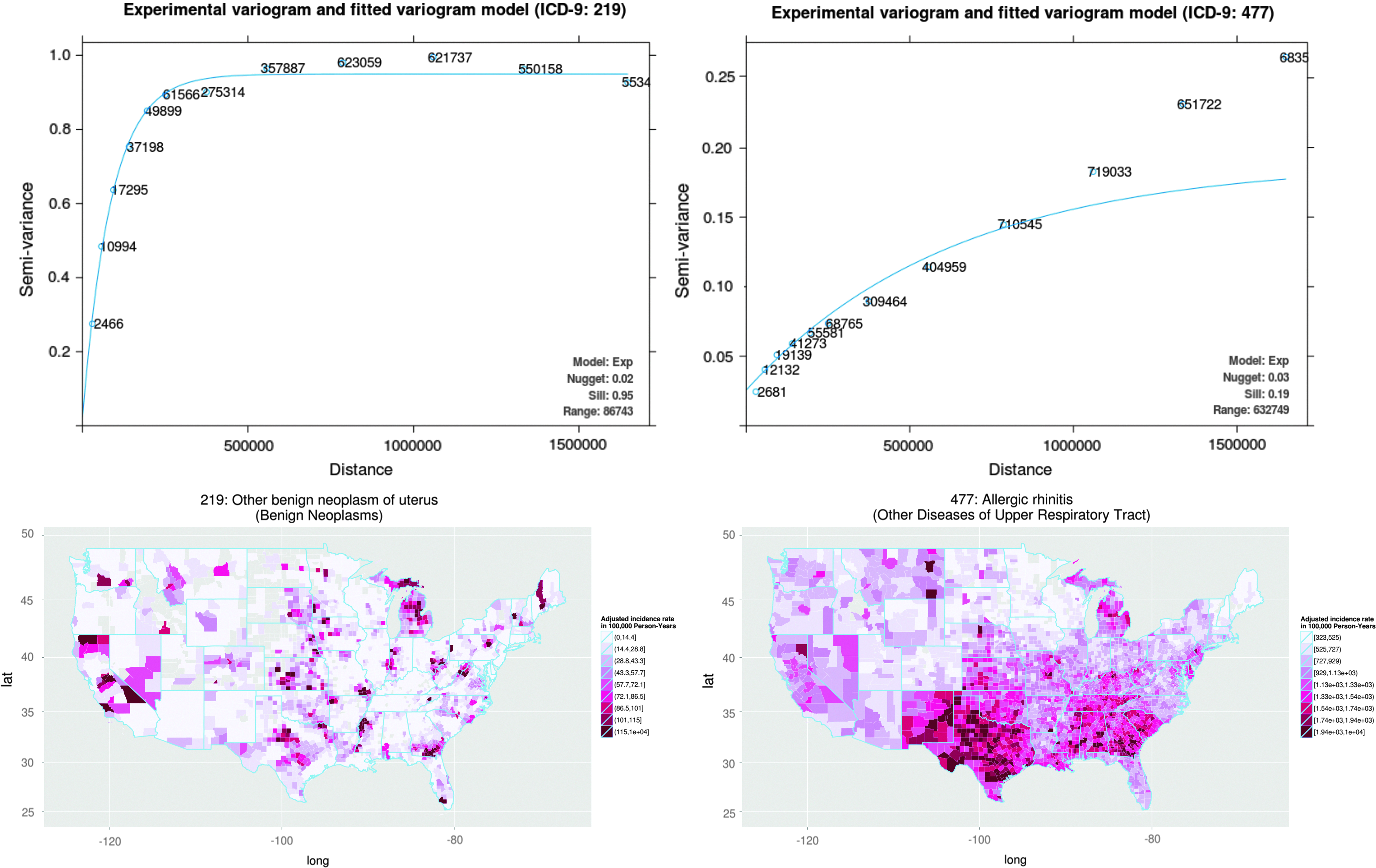
Example semivariograms and incidence rate maps for two ICD-9 codes. Top: Semivariograms for ICD-9 219, other benign neoplasms of uterus, (left) and 477, allergic rhinitis, (right). Bottom: corresponding incidence rate maps. For ease of reading, the figure can be viewed online at www.liebertpub.com/big

We compare the results of semivariogram modeling for the highest ranked ICD-9 codes using the two NB2 method implementations to the semivariogram models for the highest ranked ICD-9 codes using Moran's I statistic. Specifically, we compare average semivariogram model properties between groups of the top N ranked ICD-9 codes for increasing values of N using the two NB2 rankings and Moran's I ranking. We will refer to N as the rank threshold.

In the top of Figure 3 (left), we show the mean semivariogram range versus the rank threshold N using the NB2 method with t-test comparison (black) and Moran's I statistic (gray). This shows the average distance range within which the incidence rates are autocorrelated for the top N ranked ICD-9 codes by each method. For example, the mean semivariogram model range for the top 25 ICD-9 codes ranked by the NB2 method is 495 versus 625 km for the top 25 Moran's I statistic rankings. For the top 100 ICD-9 codes, the mean semivariogram model range is 404 and 509 km for the NB2 method with t-test comparison and Moran's I statistic, respectively. Generally, the NB2 method using the t-test comparison implementation ranks more highly ICD-9 codes showing spatial variation with smaller ranges, or smaller areas of autocorrelation.

FIG. 3.

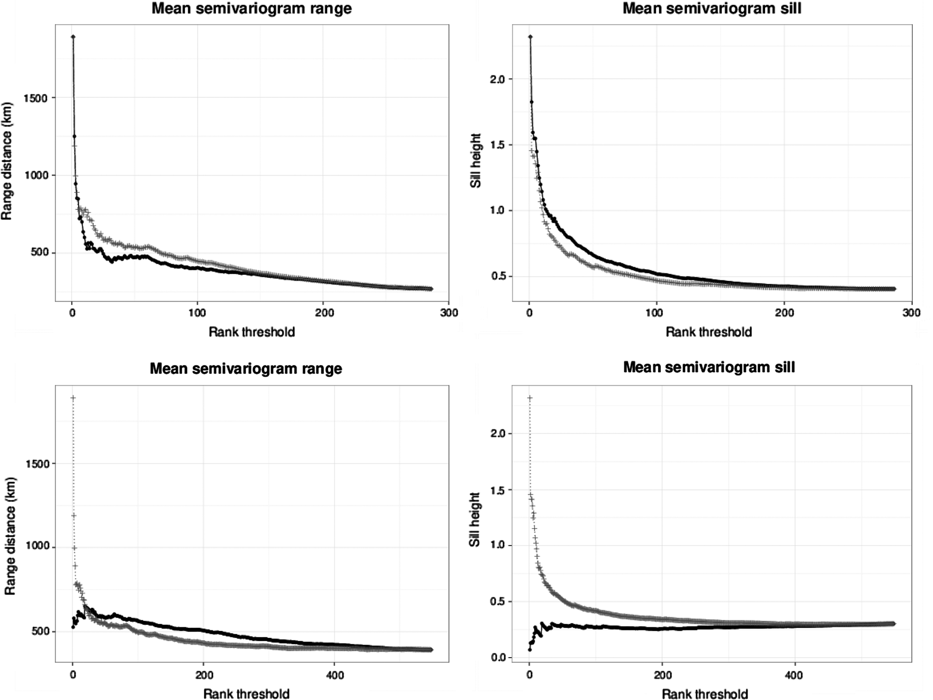
Average semivariogram properties for groups of top N ICD-9 codes by the NB2 and Moran's I methods. We show the mean range (left) and mean sill (right) for both the NB2 method (black points; top: t-test implementation, bottom: log odds implementation) and Moran's I statistic (gray crosses) plotted against the rank threshold N. Compared to Moran's I, the NB2 method with t-test implementation ranks more highly spatial variation with smaller ranges (autocorrelation within smaller distances) and larger sills (greater variance), whereas the NB2 method with log odds implementation ranks more highly spatial variation with larger ranges (autocorrelation within larger distances) and smaller sills (lower variance).

In the bottom of Figure 3 (left), for comparison we show the same plot of the highest ranking semivariogram range properties for the NB2 method with log odds comparison (black) and Moran's I statistic (gray). Generally, the NB2 method using the log odds comparison implementation ranks more highly ICD-9 codes showing spatial variation with larger ranges, or larger regions of autocorrelation.

In the top of Figure 3 (right), we show the mean semivariogram sill versus the rank threshold N using the NB2 t-test implementation (black) and Moran's I statistic (gray). This essentially shows an estimate of the average variance in incidence rates across the United States for the top N ranked ICD-9 codes by each method. For example, the mean sill for the top 25 ICD-9 codes ranked by the NB2 method is 0.85 versus 0.67 for the top 25 Moran's I statistic rankings. For the top 100 ICD-9 codes, the mean semivariogram model sill is 0.52 and 0.42 for the NB2 method t-test implementation and Moran's I statistic, respectively. In this case the NB2 t-test implementation generally ranks more highly ICD-9 codes with larger variance in the incidence rates across the United States.

In the bottom of Figure 3 (right), we show the same plot of the highest ranking semivariogram sill properties for the NB2 method with log odds comparison (black) and Moran's I statistic (gray). Generally, the NB2 method using the log odds comparison implementation ranks more highly the autocorrelated ICD-9 codes with smaller variance.

Discussion

There are many possible explanations for spatial patterns in the incidence rates of ICD-9 EMR data, and the rank ordering of ICD-9 codes with the described methods does not attempt to attribute any inferred pattern to a specific cause or suggest that the spatial variation is due to a physical environmental factor. Rather, we provide here a spatial autocorrelation method that can be implemented in multiple ways depending on the type of spatial pattern of interest. This flexibility is useful given that different categories of underlying factors as well as categories of disease can manifest as different spatial patterns, as we discuss below.

Applying the NB2 algorithm to this dataset identified various known geospatial disease patterns. For example, histoplasmosis (ICD-9 code 115) is known to be associated with bats in caves around the Ohio and Mississippi River valley,³⁷ and this pattern was picked up on the fifth row of Table 1. As another example, hypertensive heart disease (ICD-9 code 402) and essential hypertension (ICD-code 401) are known to follow a geospatial “heart failure belt.”³⁸ Hypertensive heart disease is the highest rank under the NB2 t-test in Table 1 and essential hypertension is the highest rank under NB2 using the log odds test in Table 2. On the other hand, the underlying reasons for many of the other highly ranked ICD-9 codes remains to be investigated.

Incidence levels of diseases are influenced by a variety of factors, including:

• Physical environment—Some diseases are known to be related to the physical environment.

• Socioeconomic environment—The incidence levels of some diseases are impacted by socioeconomic or regional cultural differences.

• Structural environment—The incidence levels of some diseases reflect in part geospatial differences in insurance, provider billing or reimbursement patterns, local regulations, and related factors.

We show several incidence rate maps in Figure 4 as examples of patterns corresponding to these three types. These ICD-9 codes are all ranked in the top 25 according to at least one implementation of the NB2 method. In the top left is a map showing ICD-9 code 088: Other arthropod-borne diseases, which includes Lyme disease, a disease carried by ticks and known to have a regional concentration in the northeastern United States and western Wisconsin areas. We consider this as an example of an ICD-9 code with spatial variation due to the physical environment. In the top right is a map showing ICD-9 code 635: Legally induced abortion. The spatial variation for this ICD-9 code shows clear delineation of the borders between states, which is likely to be due to differences in the structural environment. The delineation is particularly apparent on the borders between California and Nevada and New York and Pennsylvania. In the bottom left of Figure 4 is a map showing ICD-9 code 402: Hypertensive heart disease, which is the ICD-9 code ranked highest by the NB2 method. The spatial variation shows a pattern of higher incidence rate across a large crescent in the southern United States. Given this cross-state regionally concentrated pattern, we define this to be an example of differences in the socioeconomic environment. In the bottom right we show a map of ICD-9 code 763: Fetus or newborn affected by other complications of labor and delivery, which is not easily classified as the previous three examples.

FIG. 4.

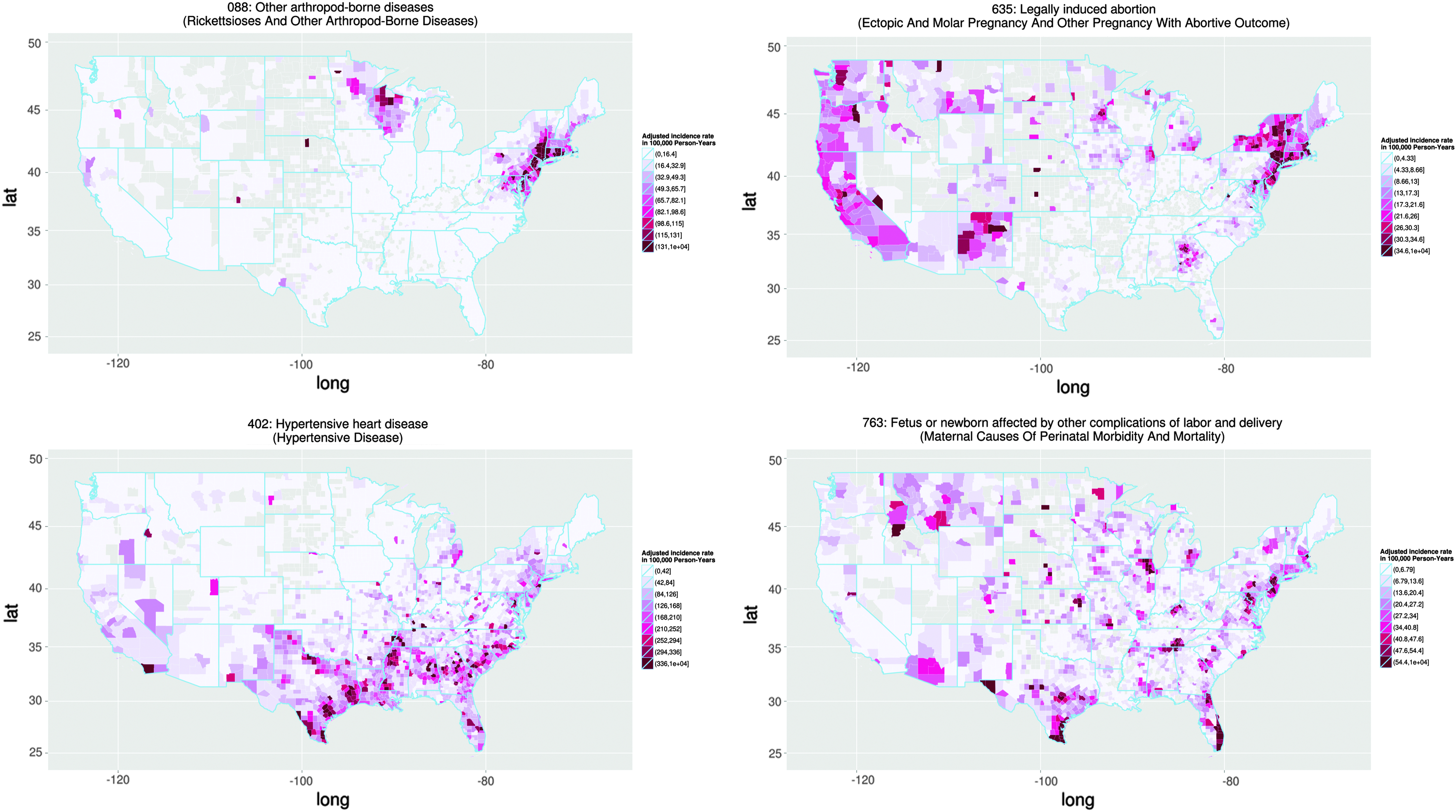
Incidence maps for several ICD-9 codes with different types of spatial variation. We show here 088: other arthropod-borne diseases (top left); 635: legally induced abortion (top right); 402: hypertensive heart disease (bottom left); and 763: fetus or newborn affected by other complications of labor and delivery (bottom right). For ease of reading, the figure can be viewed online at www.liebertpub.com/big

As can be seen from Tables 1 to 3, for patterns with hot spots that are large, well isolated, and sharply peaked (e.g., see ICD-9 code 402 in Table 1), any of the three methods rank such patterns high in the list. On the hand, for patterns that are more diffuse or with multiple smaller peaks that are closer together, the NB2 with the t-test ranks such patterns higher than Moran's I test (e.g., see ICD-9 code 763 in Table 1).

Characteristics of disease categories

In building semivariogram models describing the spatial variation for each ICD-9 code, we also looked at the model properties for categories of disease collectively. We grouped the ICD-9 codes according to standard categories, for example, 001–139 Infectious and Parasitic Diseases, 140–239 Neoplasms, etc. For each group we found the mean semivariogram model range, excluding ICD-9 codes where the semivariogram model range fit failed to iterate beyond the initial starting value, which leaves 286 individual ICD-9 codes in 17 categories. In Figure 5, we show a box plot of the semivariogram model ranges for each category ordered by increasing mean range.

FIG. 5.

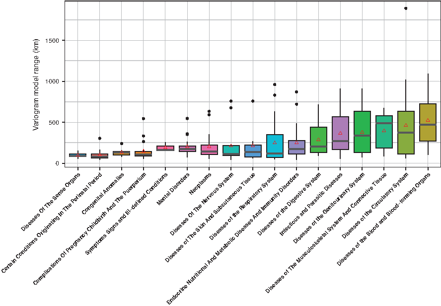
Box plot of variogram model ranges for categories of ICD-9 codes. The categories are in increasing order by the average variogram model range (marked by red triangles) for each category.

There is no correlation between the mean semivariogram model ranges of categories and the number of ICD-9 codes grouped into each category. The categories with the fewest remaining ICD-9 codes are Symptoms, Signs, and Ill-defined Conditions (three codes), Diseases of the Blood and Blood-forming Organs (six codes), and Diseases of the Skin and Subcutaneous Tissue (eight codes). The categories of Neoplasms and Infectious and Parasitic Diseases have the most codes with 29 and 26 codes, respectively. However, the diseases with the smallest ranges generally also have low mean incidence rates across the United States.

Given the variation of typical range values across different disease categories, one or the other presented implementation of the NB2 method may be appropriate for the detection of a spatial pattern for the type of disease of interest.

Conclusions

We have described here a bootstrap method that can be implemented in multiple ways for detecting patterns in spatial variation based upon a region's neighbors. The NB2 method is a procedure for quantifying how much more accurate an estimate of the value of interest is based on values from bootstrapped neighboring units than bootstrapped randomly chosen units.

We have compared two implementations of the NB2 method to Moran's I statistic for measuring spatial autocorrelation. Generally, the NB2 method and Moran's I statistic are in rough agreement although with some scatter and interesting differences. Looking at the rank orderings of ICD-9 code county incidence rates across the United States ranked by the NB2 method and by Moran's I statistic shows that, by choosing one or the other implementation of the NB2 method, we can favor spatial variation with autocorrelation within smaller distances or of larger scale. Compared with Moran's I statistic, the NB2 method allows more flexibility in controlling the type of spatial autocorrelation of interest.

Compared to Moran's I statistic, the NB2 method using the t-test comparison ranks more highly the ICD-9 codes that appear to have multiple small clusters over a region whereas the NB2 method using a log odds comparison ranks more highly the ICD-9 codes with large regional gradients. We also compared the spatial properties of categories of disease by looking at the mean fitted semivariogram properties of each category and found that different categories of disease as a whole may have larger or smaller size scales of autocorrelation, as measured by average semivariogram model ranges. For example, ICD-9 codes related to conditions originating in the perinatal period generally have spatial variation that is autocorrelated within smaller distance ranges than ICD-9 codes related to diseases of the blood and blood-forming organs. Given this difference in spatial variation scale, one or the other implementation of the NB2 method may be more appropriate depending on the category of disease.

Footnotes

Acknowledgments

This material is based in part upon work supported by the National Science Foundation under grant number 1129076 and The National Cancer Institute (NCI) under Contract NIH/Leidos Biomedical Research, Inc. 13XS021/HHSN261200800001E. This work made use of the Open Science Data Cloud (OSDC), managed by the Open Commons Consortium (OCC) and funded in part by grants from the Gordon and Betty Moore Foundation.³⁹

Author Disclosure Statement

No competing financial interests exist.

Cite this article as: Patterson MT, Grossman RL (2017) Detecting spatial patterns of disease in large collections of electronic medical records using neighbor-based bootstrapping. Big Data 5:3, 213–224, DOI: 10.1089/big.2017.0028.

Abbreviations Used

References

Friedman

, Parrish

, Ross

. Electronic health records and us public health: Current realities and future promise. Am J Public Health. 2013; 103:1560–1567.

Murdoch

, Detsky

. The inevitable application of big data to health care. JAMA. 2013; 309:1351–1352.

Brownstein

, Freifeld

, Madoff

. Digital disease detection: Harnessing the web for public health surveillance. N Engl J Med. 2009; 360:2153–2157.

Salathe

, Bengtsson

, Bodnar

, et al. Digital epidemiology. PLoS Comput Biol. 2012; 8:e100261–6.

Generous

, Fairchild

, Deshpande

, et al. Global disease monitoring and forecasting with wikipedia. PLoS Comput Biol. 2014; 10:e100389–2.

Elliott

, Wartenberg

. Spatial epidemiology: Current approaches and future challenges. Environ Health Perspect. 2004; 112:998–1006.

Rushton

, Armstrong

, Gittler

, et al. Geocoding health data: The use of geographic codes in cancer prevention and control, research and practice. CRC Press. 2007.

Beale

, Abellan

, Hodgson

, Jarup

. Methodologic issues and approaches to spatial epidemiology. Environ Health Perspect. 2008; 116:1105–1110.

Cromley

, McLafferty

. GIS and public health. Guilford Press. 2011.

10.

Noble

, Smith

, Mathur

, et al. Feasibility study of geospatial mapping of chronic disease risk to inform public health commissioning. BMJ Open. 2012; 2:e00071–1.

11.

Becker

, Glass

, Brathwaite

, et al. Geographic epidemiology of gonorrhea in Baltimore, Maryland, using a geographic information system. Am J Epidemiol. 1998; 147:709–716.

12.

Tiefelsdorf

Modelling spatial processes: The identification and analysis of spatial relationships in regression residuals by means of Moran's I (Germany). Theses and Dissertations (Comprehensive), 480, 1998. Available at: http://scholars.wlu.ca/etd/480

13.

Moran

. Notes on continuous stochastic phenomena. Biometrika. 1950; 37:17–23.

14.

Ripley

. Spatial statistics, vol. 575. Hoboken, NJ: John Wiley & Sons. 2005.

15.

Kitron

. Landscape ecology and epidemiology of vector-borne diseases: Tools for spatial analysis. J Med Entomol. 1998; 35:435–445.

16.

Hay

, Omumbo

, Craig

, Snow

. Earth observation, geographic information systems and plasmodium falciparum malaria in sub-Saharan Africa. Adv Parasitol. 2000; 47:173–215.

17.

Moonan

, et al. Using GIS technology to identify areas of tuberculosis transmission and incidence. Int J Health Geogr. 2004; 3:2–3.

18.

Sasaki

, Suzuki

, Igarashi

, et al. Spatial analysis of risk factor of cholera outbreak for 2003–2004 in a peri-urban area of Lusaka, Zambia. Am J Trop Med Hyg. 2008; 79:414–421.

19.

Kamadjeu

. Tracking the polio virus down the congo river: A case study on the use of Google earth? In public health planning and mapping. Int J Health Geogr. 2009; 8:4.

20.

Nuckols

, Ward

, Jarup

. Using geographic information systems for exposure assessment in environmental epidemiology studies. Environ Health Perspect. 2004; 112:1007–1015.

21.

Weis

, Balshaw

, Barr

, et al. Personalized exposure assessment: Promising approaches for human environmental health research. Environ Health Perspect. 2005; 113:840–848.

22.

Huang

Y-L

, Batterman

. Residence location as a measure of environmental exposure: A review of air pollution epidemiology studies. J Expo Anal Environ Epidemiol. 1999; 10:66–85.

23.

Jarup

. Health and environment information systems for exposure and disease mapping, and risk assessment. Environ Health Perspect. 2004; 112:995–997.

24.

Graves

. Integrative literature review: A review of literature related to geographical information systems, healthcare access, and health outcomes. Perspect Health Inf Manag. 2008; 5:5–11.

25.

Dean

, Fenton

. Addressing social determinants of health in the prevention and control of HIV/AIDS, viral hepatitis, sexually transmitted infections, and tuberculosis. Public Health Rep. 2010; 125:1.

26.

Harrison

, Dean

. Use of data systems to address social determinants of health: A need to do more. Public Health Rep. 2011; 126:1.

27.

Gatrell

, Elliott

. Geographies of health: An introduction. West Sussex, UK: John Wiley & Sons. 2014.

28.

Luther

, Studnicki

, Kromrey

, et al. A method to measure the impact of primary care programs targeted to reduce racial and ethnic disparities in health outcomes. J Public Health Manag Pract. 2003; 9:243–248.

29.

Geraghty

, Balsbaugh

, Nuovo

, et al. Using geographic information systems (GIS) to assess outcome disparities in patients with type 2 diabetes and hyperlipidemia. J Am Board Fam Med. 2010; 23:88–96.

30.

Comer

, Grannis

, Dixon

, et al. Incorporating geospatial capacity within clinical data systems to address social determinants of health. Public Health Rep. 2011; 126:5–4.

31.

Rodriguez

, Hotchkiss

, O'Hare

. Geographic information systems and chronic kidney disease: Racial disparities, rural residence and forecasting. J Nephrol. 2013; 26:3.

32.

Rzhetsky

, Bagley

, Wang

, et al. Environmental and state-level regulatory factors affect the incidence of autism and intellectual disability. PLoS Comput Biol. 2014; 10:e100351–8.

33.

Klein

, Schoenborn

. Age adjustment using the 2000 projected us population. Healthy People Statistical Notes. Hyattsville, MD: National Center for Health Statistics, 2001; 20.

34.

Day

. Population projections of the United States, by age, sex, race, and Hispanic origin: 1992 to 2050. 1092, US Department of Commerce, Economics and Statistics Administration, Bureau of the Census. Washington, DC, 1992.

35.

Waller

, Gotway

. Applied spatial statistics for Public Health data, vol. 368. Hoboken, NJ: John Wiley & Sons. 2004.

36.

Bivand

, Pebesma

, Gómez-Rubio

. Applied spatial data analysis with R. New York: Springer. 2013.

37.

Benedict

, Mody

. Epidemiology of histoplasmosis outbreaks, United States, 1938–2013. Emerg Infect Dis. 2016; 22:37–0.

38.

Mujib

, Zhang

, Feller

, Ahmed

. Evidence of a “heart failure belt” in the southeastern united states. Am J Cardiol. 2011; 107:935–937.

39.

Grossman

, Greenway

, Heath

, et al. The design of a community science cloud: The open science data cloud perspective. In: SC Companion, IEEE Computer Society, 2012. pp. 1051–1057.

Supplementary Material

Please find the following supplemental material available below.

For Open Access articles published under a Creative Commons License, all supplemental material carries the same license as the article it is associated with.

For non-Open Access articles published, all supplemental material carries a non-exclusive license, and permission requests for re-use of supplemental material or any part of supplemental material shall be sent directly to the copyright owner as specified in the copyright notice associated with the article.

0.00 MB

0.07 MB

Detecting Spatial Patterns of Disease in Large Collections of Electronic Medical Records Using Neighbor-Based Bootstrapping

Abstract

Abstract

Introduction

Materials and Methods

Data

NB2 method

Results

Performance

Comparison with Moran's I statistic

Scale of spatial influence

Discussion

Characteristics of disease categories

Conclusions

Footnotes

Acknowledgments

Author Disclosure Statement

Abbreviations Used

References

Supplementary Material