
Abstract
Abstract
One of the most challenging problems facing crime analysts is that of identifying crime series, which are sets of crimes committed by the same individual or group. Detecting crime series can be an important step in predictive policing, as knowledge of a pattern can be of paramount importance toward finding the offenders or stopping the pattern. Currently, crime analysts detect crime series manually; our goal is to assist them by providing automated tools for discovering crime series from within a database of crimes. Our approach relies on a key hypothesis that each crime series possesses at least one core of crimes that are very similar to each other, which can be used to characterize the modus operandi (M.O.) of the criminal. Based on this assumption, as long as we find all of the cores in the database, we have found a piece of each crime series. We propose a subspace clustering method, where the subspace is the M.O. of the series. The method has three steps: We first construct a similarity graph to link crimes that are generally similar, second we find cores of crime using an integer linear programming approach, and third we construct the rest of the crime series by merging cores to form the full crime series. To judge whether a set of crimes is indeed a core, we consider both pattern-general similarity, which can be learned from past crime series, and pattern-specific similarity, which is specific to the M.O. of the series and cannot be learned. Our method can be used for general pattern detection beyond crime series detection, as cores exist for patterns in many domains.
Introduction
One of the most important problems in crime analysis is that of crime series detection, or the detection of a set of crimes committed by the same individual or group. Criminals follow a modus operandi (M.O.) that characterizes their crime series; for instance, some criminals operate exclusively during the day, others work at night, some criminals target apartments for housebreaks, while others target single family houses. Crime analysts need to identify these crime series within police databases at the same time as they identify the M.O. Currently, analysts identify crime series by hand: They manually search through the data using database queries trying to locate patterns, which (as Ref. notes) can be very challenging and time-consuming. From a computational perspective, crime series detection is a very difficult problem: It is a clustering problem with cluster-specific feature selection, where the set of features for the cluster is the M.O. of the criminal(s). One cannot know the M.O. of the series without determining which crimes were involved, and one cannot locate the set of crimes without knowing the M.O.—the M.O. and the set of crimes need to be determined simultaneously. Pattern analysis for crime has existed at least as far back as the 1840s, 2 but recently, big data has changed the whole landscape for crime analysis. To locate crime patterns, analysts now rely on large amounts of very detailed data about large numbers of past crimes. The computational problem of finding crime series grows exponentially with the numbers of crimes and features of crimes. Even if a crime analyst could identify crime series within his/her own department database (which is already difficult), these manual efforts cannot scale, for instance, when neighboring police departments start to combine databases.
Despite its critical importance for public safety, there is little in the way of tools to help police. Most predictive policing software has the capability to detect only general background levels of crime density in time and space, which are much easier to predict than specific patterns of crime. This is called hotspot prediction, and it requires only time and location data, and a density estimation algorithm: Crimes are predicted to occur based on where and when they occurred in the past. No detailed information about the M.O. of the crimes is used for hotspot prediction, and hotspots can involve crimes committed by different offenders (as opposed to crime series, which have the same offenders). In fact, at least in the case of Cambridge, Massachusetts, crime series generally do not take place in hotspots (see also Ref. 3 for a study of crime series in two other U.S. cities). Hotspot prediction software is not what we need for the problem of crime series detection.
The problem of crime series detection is much more data intensive and computationally harder than hotspot prediction. To determine the M.O., we require very fine-grained detailed information about past crimes: where the offender(s) entered (front door, window, etc.); how they entered (pried doors, forced doors, unlocked doors, pushed in air conditioner, etc.), whether they ransacked the premise, the type of premise, etc. This is high dimensional structured data, leading to a computationally challenging data mining problem of finding all crimes that are similar to each other in several ways.
Crime series detection results can be used for many purposes. First, if a pattern is identified, investigative resources can be prioritized to focus on the crime series, to gather and assemble evidence. For instance, video recordings from nearby streets and stores or banks can be examined for evidence of the offender's location with respect to all crimes in the series, and combined with suspect descriptions from witnesses (if any). Call-detail records from cell phones can also be used for this purpose, as well as latent fingerprints and tracking information from stolen property. Second, if a current crime series is localized enough to have predictable times and locations (for instance, a pickpocket targeting a single café at regular intervals throughout the week), actions can be taken to stop the pattern. Third, if a current crime series has the same M.O. as a past crime series for which the offender is known, then the suspect from the older series could be a potential offender for the current crime series. Fourth, crime series detection results can be used to study criminal behavior generally. There is strong evidence that a majority of crimes are committed by a small number of serial criminals, 4 which underscores the importance of identifying and studying the patterns of serial offenders.
Conversely, we remark that nothing can be done if police do not know that a pattern is occurring at all. Without the capability of automatically detecting a specific series of crime, it is possible that crime series may take much longer to identify, or may never be identified. This is especially problematic for certain types of crime—for instance, for housebreaks (burglaries) there is often no suspect information since the crimes take place when residents are not present. Housebreaks can be extremely difficult crimes to solve, and nationwide only 14% of housebreaks are solved. 5 In this article, we aim directly at identifying series in housebreaks in an automated way.
The main hypothesis in this work is that most crime patterns have a core of crimes that exemplify the M.O. of the series. A core might be approximately three or four crimes that are very similar to each other in many different ways. According to our hypothesis that each crime series has a core, if we can locate all small cores of crime within the dataset, we have thus located pieces of most crime series. This hypothesis is based on the intuition of analysts and has the dual purpose of assisting with computation: We can indeed consider all reasonable small subsets to calculate whether they are plausible cores.
Though we cannot determine the M.O. of a series before we see it, we can characterize parts of the M.O.s we expect generally—for instance, crimes in a series are often close in time and space. We define a pattern-general similarity that encodes factors that are generally common to most crime series. It is learned from past crime series; for instance, proximity in time and space highly contribute to the pattern-general similarity. The pattern-general similarity induces a similarity graph over the set of crimes, where there is an edge between two crimes when they are similar according to the pattern-general similarity.
Crimes in a series also have pattern-specific similarity, where crimes are similar to each other if they all share the same M.O. The pattern-specific similarity and pattern-general similarity (the similarity graph in particular) are used for detecting cores: A core must have both sufficiently large pattern-general similarity and pattern-specific similarity. The cores are found using an integer linear programming (ILP) formulation. Once the cores are found, we construct the full crime series by merging overlapping cores. We also prove that merging cores preserves desired properties.
Our method is a general subspace clustering method that can be used beyond crime series, and for other completely different application domains. It is novel in that it considers both pattern-general and pattern-specific aspects of patterns, where “pattern-general” means that it is common to many crime series (supervised from past clusters), and “pattern-specific” meaning aspects of a particular crime series (unsupervised). Our method does not force all examples to be part of a cluster and can thus accommodate background (non-series) crime. Our method also can find subspace clusters whose subspace morphs dynamically over the cluster; an M.O. can change when an offender becomes more sophisticated, adapts his M.O. to avoid detection, or when his preferred method is not available (e.g., he prefers entry through unlocked rear doors but will push in the air conditioner if his preferred means of entry is not available).
This project highlights several important aspects of big data analytics. It highlights an emphasis on human collaboration within the analysis pipeline, which is a key challenge for big data (see, for instance, the CCC white papers 6 ). This project also exemplifies a separate challenge, namely that of increased complexity. Once our problem is formulated, solving it requires a combinatorially hard optimization problem and an explosion of variables. We could, for instance, add a “V” for “Variables” to the traditional V's of big data in order to capture problems that require massive computation to solve a problem of increased complexity. The big data challenge of problems with increased complexity has arisen in other places (see, for instance, the American Statistical Association's white paper on big data 7 ).
Our three methodology sections follow the three main components of our method: learn a similarity graph, mine cores, and merge cores. We then show experiments where our method was tested on the full housebreak database from the Cambridge Police Department containing detailed information from thousands of crimes from over a decade. This method has been able to provide new insights into true patterns of crime committed in Cambridge. One observation that has been revealed in our experiments is that computers do not have the same biases that humans do. Computers search through the database in a different way than a human would, and thus can work symbiotically with analysts, showing them avenues to consider where they would not have normally ventured.
Related work
There are at least three main types of recent approaches to identifying crimes committed by the same individual or group (according to Ref. 8 ).
The first approach, sometimes known as pairwise case linkage, involves identifying whether a pair of crimes was committed by the same group, where each pair is considered separately. Some of these works use weights determined by experts9–12 to weight the various types of similarities between crimes, and other works learn the similarity weights from data.13–23 The problem with considering only pairwise linkages is that only one similarity measure between crimes is used. This has a fundamental flaw that it does not consider M.O.'s of individual crime series. Consider two crime series with different M.O.'s: one has an M.O. in which the means of entry is to push in an air conditioner on a ground floor apartment (in buildings that are not concentrated geographically), and the M.O. of the other crime series involves breaking into a single family home at night (not using a consistent entry method) while the residents are present in a small geographical area. If we are investigating whether a new crime fits into the first series, logically we should consider whether the suspect entered by pushing in an air conditioner of an apartment and we should not consider geographical area. When we are investigating the second series, we should consider geographical area, time of day, and whether residents were present; we should not consider means or location of entry. If we use a single measure to judge similarity between any two crimes (as in pairwise case linkage approaches), it is not possible to make this distinction. In pairwise linkage approaches, it is not possible to ignore certain types of information about similarity and pay attention to others, as we claim is necessary for understanding multiple different M.O.'s. As a result, these approaches generally find that time and space are the only relevant dimensions for this type of analysis (see for instance Ref. 20 ), and end up ignoring the detailed behavioral information.
The second type of approach is called reactive linkage, where a crime series is discovered one crime at a time, starting from a seed of one or more crimes (as defined by Refs.1,8). Reactive linkage has a similar problem to pairwise linkage in that when we start to grow a set of crimes greedily from a small seed of one or two crimes, we cannot yet know the M.O. of the crime series. This means that yet again we start from a common similarity metric between crimes. The greediness of this approach, coupled with the fact that the distance metric does not take into account the M.O., could lead to problematic results. Our past approach to this24,25 did use a theoretically motivated 26 greedy method, but adapted the distance metric to be closer to the observed M.O. as more crimes were added to the set. This still does not solve the problem of greediness, and the result could depend on which crimes were used as seed crimes. On the other hand, these greedy methods are very computationally tractable.
In the last type of approach, crime series clustering, all the clusters are found simultaneously.8,27–35 One of the earliest approaches we know of for clustering crimes is that of Dahbur and Muscarello, 29 who used a neural network approach. (This method had some serious flaws that required extensive heuristic post-processing after the clusters were created, but aimed at solving the more general problem of crime clustering.) Most of these approaches use a form of hierarchical clustering, which again has the disadvantage that the distance metric between crimes is static and does not reflect the M.O. of any particular crime series. (On the other hand, hierarchical clustering is very computationally tractable and could be made to reflect pattern-general similarity, though not pattern-specific similarity.) Some of these approaches reduce features one at a time through hypothesis tests, or use basic dimensionality reduction (multidimensional scaling) techniques before clustering. This still does not handle pattern-specific aspects, and thus, cannot capture the M.O.
A main point of the present work is that in order to model the M.O., we need to use some form of subspace clustering. The M.O. for the pattern is precisely the subspace; it is the set of dimensions for which crimes in a particular series should be considered to be similar. For the first crime series in the example above, we would consider mainly the subspace “means of entry” involving the entry by pushing in air conditioners, and we would not heavily consider the dimension for geographical area. The algorithm must determine which observations go into which cluster, and which subspace is relevant for each cluster. Our work relates to various subfields of clustering (see, for instance, Ref. 36 ), including pattern-based clustering,37,38 which is a semi-supervised approach (unlike ours—we do not use test data at training time); general subspace clustering (e.g., Refs.39,40), which detects all clusters in all subspaces; and work at the intersection of dense subgraph mining and pattern mining in feature graphs.41,42 These methods would not be able to take into account the complexities we handle, for instance, learning the pattern-general weights, or finding cores with the characteristics we require. Other work on space-time event detection is relevant,43,44 where the goal is to detect patterns such that the frequency of records is higher than an expected frequency. A relevant method for clustering with simultaneous feature selection is that of Guan et al., 45 which is similar to our core detector in flavor, although feature selection is controlled differently, and there are no pattern-general aspects.
Reviews of other data mining applications in crime analysis are those of Chen et al. 46 and Thongtae and Srisuk. 47 There are several other works that use machine learning for various criminology applications.48–50
Model Formulation
Our data consist of entities (crimes)
Define sj to be a symmetric similarity function on the jth feature sj : Dj×Dj→[0, 1], where sj(vl, vk) measures the similarity between crimes vℓ and vk in the jth feature. In our case most features are categorical, some are ranges, and some are spatial coordinates. For instance, if two crimes have location of entry as “window,” then they would get a high location-of-entry similarity. The similarity measures are discussed in depth in our earlier work,24,25 so we will not go into detail here. The average similarity of a set of crimes in feature j is defined as the cohesion of the set:
The defining features of a pattern are those with sufficiently high cohesion.
The defining features characterize the M.O. of the crime series. If several housebreaks happen in the same neighborhood, around the same time of day, within the same month, and the location of entry is always a window, regardless of the differences in other features, these similarities would indicate that the crimes could have been committed by the same offender. The features “geographic location,” “time of day,” “time between crimes,” and “location of entry” characterize the M.O. for this particular crime series. When we later define cores, the pattern-specific statistic of interest is the number of defining features of V.
Let us switch from pattern-specific definitions to pattern-general definitions. We will learn a pattern-general similarity function from past crime series. Pattern-general similarity allows us to weight important features highly; for instance, crimes that are spread very far apart in time and space are unlikely to be a pattern, and thus we will learn from past crime series that time and space are important features. We will learn a set of weights
Our cores will also be connected in the similarity graph. To construct edges for the graph, we first define a metric to measure the similarity between two crimes, as follows:
We define the similarity graph to contain edges between crimes that are sufficiently close in the pattern-general sense.
For us to even consider whether V should be a core of a series, the core needs to be connected in the graph theoretic sense (and is not composed of two separate clusters for instance), must have sufficient connectivity, and must have sufficiently high pattern general cohesion. The requirement that a core must be a connected set means that each crime in a core must be similar in pattern-general similarity to at least one other crime in the core.
We learn both the weights {λj} j and cut-off threshold Δ from data, as discussed in Section 3 below, in order to perform the first piece of the method, which is to construct the similarity graph. Note that we could eliminate the first piece of the method, and eliminate the pattern-general similarity all together by setting the threshold Δ to be very low, and that way we consider only pattern-specific similarity; this, however, would not ease computation or restrict the cores to be similar to those from other patterns. Imposing a graph structure on the crimes eases computation, in the sense that we are now only looking for connected sets of the graph when we mine for cores in the second part of the method.
The second part of the method is to mine for cores. When we mine for cores, we cannot simply maximize the number of defining features and/or the pattern-general cohesion over all subsets of crime, as it would favor choosing very small sets of crime as cores. To alleviate this problem, we specify the size of the core |V | and the number of defining features d, and find cores that maximize the pattern-general cohesion. Once we find the cores, we merge them to find the rest of the pattern. We call patterns formed by merging other patterns together serieslike patterns. An illustration of a serieslike pattern is shown in Figure 1.
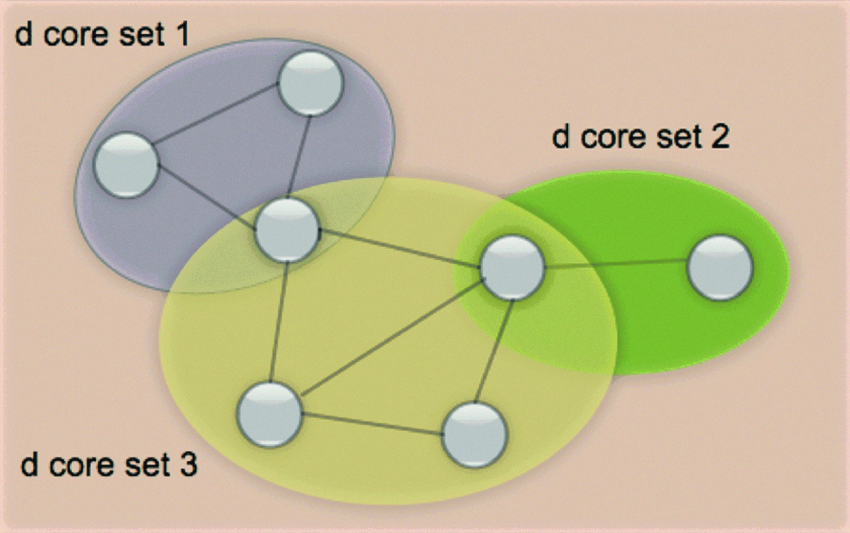
A d serieslike pattern consisting of three d cores of various sizes.
Learning the Similarity Graph
As we discussed, the similarity graph is constructed by connecting pairs of nodes with pattern-general cohesion above a threshold Δ. The pattern-general cohesion γ is defined in (1) as a weighted sum of pairwise similarities in different features, with pattern-general weights
To learn the weights, we optimize over the historical training patterns to make them as close as possible to being connected subgraphs. This means we want each crime in a historical pattern to be close to at least one other crime in the same pattern. At the same time, we want crimes within a historical pattern to be distant from crimes not in the same pattern. The condition for crime ℓ to be close to at least one other crime within its pattern (with some slack εℓ) is:
Conversely, crimes that do not belong to the same pattern should not be very similar:
true for all ℓ and k such that
where ∥
We propose a mixed-integer programming (MIP) formulation for solving this. In what follows, decision variables yℓk are binary, and they select a crime k that is most similar to a given crime ℓ within the same pattern. That is, they encode the max from constraint (2). The formulation is:
such that
Constraint (4) comes from (2). It forces yℓ,k to be chosen correctly so that if k is the crime closest to ℓ, then yℓ,k will be 1. This is because εℓ is minimized within the objective, so yℓ,k is necessarily going to correspond to the index where εℓ is minimized, and where the similarity is maximized within (4). Constraints (5) and (6) further define yℓ,k's by stating that a crime in the pattern needs only to be connected to one closest neighbor ℓ in the pattern (this is the requirement of connectivity), and its entries are binary. Constraint (7) comes from (3). The value ∑jβj is the ℓ0 norm of
Cores
A d-core is a set of crimes that exhibit similarity in a feature subspace of d dimensions. A d-core has d defining features that are not predetermined. Further, crimes in a d-core need to be well connected in the similarity graph. Formally, the definition is as follows.
• Pattern specific constraint: the size of the defining feature set of the graph is equal to d, |Λ(G)|=d.
• Pattern general constraints: G is connected, and G is dense,
Two parameters, d and α, control the property of the core in a pattern-specific and pattern-general way, respectively.
The pattern-general constraints should be thought of as being much looser than the pattern-specific constraints, as we often include unnecessary edges in the similarity graph. For the set of crimes to be feasible in the pattern-specific sense is much more difficult, as crimes in the pattern need to be similar to each other in d separate ways.
We find cores G=(V, E) using an optimization method to maximize the pattern-general cohesion while satisfying the core constraints.
We propose a binary integer linear formulation for the optimization problem (12). Let
where matrix
Let us derive the objective. Since
The objective is the pattern-general cohesion. Equation (13) ensures that the cores we discover are of size n. Constraints (14), (15), and (16) are the pattern-specific constraints. Constraint (14) forces dj=1 when Cohesion
j
(G)≥θj, where the strict inequality is enforced by ε. Constraint (15) forces dj=0 when Cohesion
j
(G)<θj. Constraint (16) specifies the number of defining features as d. The symmetry of
Expression (20) is a pattern-general constraint. Our formulation does not enforce the core to be connected, but it does enforce something weaker, namely that each node in a core of size n is at most n − 1 steps along the similarity graph from any other node in the core. We handle the connectivity afterward by examining the result to ensure that it is connected and labeling it as infeasible if not. To handle the constraint that each node in the core is at most distance n − 1 from every other node, we recall that in graph theory, if node vk is reachable from node vℓ in exactly q steps,
Thus, (20) forces that if vℓ and vk are both in the pattern, they must be at most distance n – 1 along the graph.
The pattern-general density constraint is handled similarly to the connectivity constraint, where feasibility is checked for each solution, and infeasible solutions are removed.
The integer program finds one solution at a time. In order to avoid finding a solution that was found previously, we introduce a constraint for each previous solution found. Suppose in the t-th run, the crimes in the solution are
This constraint will exclude the current solution from the feasible region, and we will obtain a different solution in the next run if any feasible solutions remain. Since all of the matrices are symmetric, in practice we keep only the upper (or lower) triangle, including the diagonal, to compute all of the sums.
Merging Cores
By our main hypothesis, the vast majority of crime series contain a core. This means that by finding all cores, we would have located the vast majority of all crime series. We now grow the rest of the crime series from the cores by merging them together. One advantage of merging is that it allows the pattern to dynamically change, as the defining features from the merged cores are not always equal to each other. Consider a burglar's M.O. with a shifting means of entry. At first he enters through unlocked doors, then he starts to use bodily force to open doors, and later he learns to use a screwdriver to pry the door open. His full pattern thus consists of several smaller d-cores. This suggests a more flexible definition of pattern than a simple core. We provide such a definition below.
• Pattern general constraint: G is connected.
• Pattern specific constraint: Each node u in G is contained in at least one subgraph G′⊆G that is a d′-core with defining features that include set Π(G), that is, Π(G)⊆Λ(G′), d≤d′.
Note that if a graph is a d-serieslike pattern, it is also a (d– 1)-serieslike pattern, a (d – 2)-serieslike pattern, and so on. The pattern specific constraints for d-serieslike patterns are looser than those for d-cores. A d-serieslike pattern may not be a d-core. On the other hand, a d-core is a special case of a d-serieslike pattern. Before we proceed, we must ensure that merging is justified.
This leads directly to the following:
Then
These properties lead to the following breadth first search algorithm for mining d-serieslike patterns. We start with the cores that we found using the integer program. These cores are candidates for merging. We also maintain an active pattern set that contains the d-serieslike patterns that we are not done constructing. We keep the d-serieslike patterns that we are done constructing in a maximal pattern set. To start, the active pattern set contains all of the d-cores we found. For each active pattern, we iterate through the candidates to see if they meet the merging criteria provided just below. If a merge is possible, and if the merged set had not been previously created, we append the merged pattern to the active pattern set and continue iterating through the candidates. If there are no candidates that can be merged with the active pattern at all, then the active pattern is maximal, and it is placed in the maximal pattern list. The merging criteria for G1∪G2 to form a d-serieslike pattern
• G1∩G2≠
• |Π(G1)∩Π (G1)|≥d.
The merging algorithm is formulated in Algorithm 1.
Experiments
Our data set was provided by the Crime Analysis Unit of the Cambridge Police Department in Massachusetts. It has 7,067 housebreaks that happened in Cambridge between 1997 and 2011, containing 51 hand-curated patterns contained within the 4,864 crimes between 1997 and 2006. (Patterns from 2007 to 2012 were not assembled at the time of writing.) Crime attributes include geographic location, date, day of week, time frame, location of entry, means of entry, an indicator for “ransacked,” type of premise, an indicator for whether residents were present, and suspect and victim information. The 51 crime series identified by police contain an average of 12.1 crimes each, with the largest series containing 59 crimes, and the smallest series containing 2 crimes. These crimes span an average period of 42 days, with the shortest series taking place within 1 day and the longest series taking 451 days. Data were processed using the similarity functions {sj}
j
discussed in our previous work,24,25 where each pairwise feature is mapped into a number between 0 and 1. These similarity measures are p-values, and they consider the baseline frequency of each possible outcome for the categorical variables. For instance, most crimes are committed when residents are not present. If two crimes were committed where one had residents present and the other had residents that were not present, then the similarity score for “residents present” is zero. If both crimes were committed when the residents were not present, the similarity score for “residents present” would not be high (in particular, it is
Baselines
As this problem is fundamentally a clustering problem, we compare with several varieties of hierarchical agglomerative clustering and incremental nearest neighbor approaches. For these baselines, we use several different schemes to iteratively add discovered crimes, starting from pairs of nodes with high similarity γ, which is a weighted sum of the attribute similarities:
Unlike our method where the weights are learned, the weights
Hierarchical agglomerative clustering (HAC) begins with each crime as a singleton cluster, and iteratively merges the clusters based on the similarity measure between clusters. Nearest neighbor classification (NN) first selects pairs of crimes with high similarity and then iteratively grows a cluster by adding the nearest neighbor crime to the cluster.
HAC and NN were used with three different criteria for cluster–cluster or cluster–crime similarity: single linkage (SL), which considers the most similar pair of crimes; complete linkage (CL), which considers the most dissimilar pair of crimes; and group average (GA), which uses the averaged pairwise similarity.
51
When the nearest neighbor algorithm is used with the SGA measure defined below with weights provided by crime analysts, it is similar to the Bayesian Sets algorithm and how it is used for set expansion.52,53
Evaluation metrics
There are two levels of performance we evaluate - pattern-level and object-level.
Pattern-level precision and recall
We evaluate the quality of the core detector using pattern-level precision and recall. The d-cores are smaller as d becomes larger. The cores are used for discovering larger merged patterns. Thus we evaluate the accuracy of the core finder in its detection ability; if a real pattern is missed completely by our core detector, there is no way to recover from this in order to detect it. If a core covers more than one pattern, this is also a bad seed for further mining, since it would generate misleading defining features that do not characterize any real patterns. Thus, we call cores that cover one and only one real pattern good cores. The pattern-level precision and recall are both defined using good cores. N denotes the number of cores we discover.
Note that pattern-level precision should be large, as each real pattern should contain many cores, inflating the reported precision values.
Object-level precision and recall
We evaluate the full pipeline for generating serieslike patterns using object-level precision and recall. To do this, for each pattern discovered, we determine how close it is to one of the real patterns. If the discovered pattern overlaps only one real pattern, then we call this the dominating pattern and evaluate precision and recall with respect to crimes in that pattern. If the serieslike pattern overlaps more than one real pattern, we assign the dominating pattern to be the real pattern possessing the most crimes that overlap with our discovered pattern. Note that it is possible for the recall not to grow with the size of the discovered pattern, as the dominating real pattern could change as the discovered pattern grows larger. The definitions of object-level precision and recall for a d-serieslike pattern G=(V, E) are as follows:
where |Vdominating pattern| is the number of crimes in the dominating real pattern.
Computational gain from similarity graph
The first step in our method is to learn the similarity graph. The similarity graph provides a computational gain in that it creates constraints on possible cores, reducing the feasibility region of the ILP. For this similarity graph, recall that we desire crimes in the same real pattern to be connected to each other. We call edges connecting crimes that belong to the same pattern good edges. If we have constructed the similarity graph well, the similarity graph should have a higher percentage of good edges than if we had simply used the full graph consisting of all possible edges. If we remove a few good edges in the process, this is not problematic as long as the true patterns are still connected in the similarity graph—this will be assessed when we assess the quality of the cores and the full pipeline next.
Table 1 shows the percentages of good edges in both the similarity graph and the full graph for four test folds (the data were divided into four folds, and each was used in turn as the test fold). The learning method tends to reduce the number of unnecessary edges by a factor of 7 or 8 in each of the test folds, as shown in the third column (which is the first column divided by the second column). This reduction substantially reduces computation for the core finder.
Pattern-general weights
The pattern-general weights come from the learning step for the similarity graph. In Figure 2 we report the mean over the test folds of the pattern-general weights we discovered. The highest weights are similarity in distance, number of days apart, suspect information, whether residents are present, and means of entry (e.g., pried, forced, cut screen).
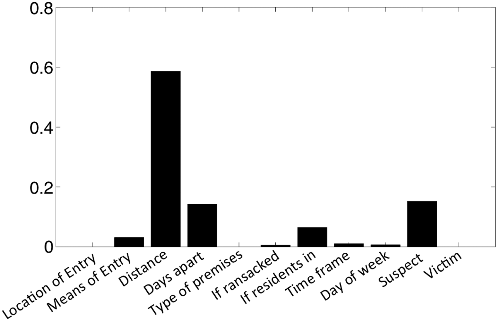
Pattern-general weights.
Time windowing
Consider solving the ILP for finding cores on data from 4,864 housebreaks. Note that if we were to search for patterns of size 10 among 1,000 crimes, this would mean investigating
Because the pattern-general weight on closeness in time is so high, we determined that we would be unlikely to miss true cores if we considered windows of time that include at least 200 crimes. We thus indexed the housebreak records in chronological order and created overlapping windowed blocks of 200 crimes each, where neighboring blocks have an overlap of 100 crimes. Therefore we solve ILPs among crime subsets
Evaluation of mining cores
We chose performance evaluation metrics from information retrieval, and for some of these metrics, we need to rank the discovered cores by a scoring function. This scoring function represents how certain we are that these cores are real. We use a scoring function that is a weighted version of pattern-general cohesion and the (pattern-specific) number of defining features, as we desire cores that are both tight in the pattern-general sense and in the pattern-specific sense. Here is the score function:
Series usually have about six defining features, so the choice of 1/6 tends to balance the two terms, weighing the pattern-specific term slightly higher. We ordered the discovered cores in decreasing order of the scores. Note that the first evaluation below does not require these scores, but the second and third do.
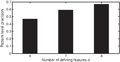
Pattern-level average precision of d cores of different sizes.
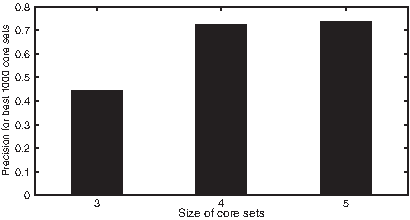
Pattern-level precision of cores with different sizes.
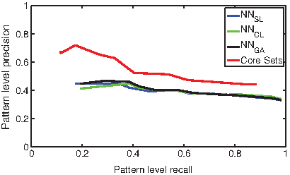
Average pattern-level precision vs. recall.
Evaluation for mining serieslike patterns
We evaluated the quality of our full pipeline and the baseline methods as follows. After all the serieslike patterns were discovered, we evaluated the average object-level precision and recall for all the patterns and over all the test folds, plotted as a point on Figure 6. For HAC, we simply iterated it, stopping at a threshold where recall was approximately equivalent to our method, and again reported average object-level precision and recall on Figure 6. For the nearest neighbor method, after each element was added to a growing pattern, we evaluated precision and recall to trace out a precision-recall curve. All three metrics in (24) were used for HAC and nearest neighbors. We note that for the same level of recall, the precision attained by our method was quite a bit higher than that of other methods.
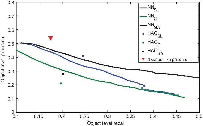
Object-level precision and recall.
There is still a lot of room for improvement. Currently, with precision on the order of 53%, we capture approximately 18% of the crimes identified by analysts. That is, when our method returns a crime, it is a real crime in a series about 53% of the time. We are returning about one-fifth of the crimes at these settings, so our method currently is conservative–it will not claim that a crime is in a series unless it is reasonably certain. This can help ensure that analysts do not overlook crimes that are very likely to be in a particular series. Note that our ground truth consists of crime series that are hand-labeled by analysts, and these labels are not perfect. For instance, it is entirely possible that we return crimes that are in a series that the police had not previously considered. We might opt to change the settings so that the method returns more crimes as being potentially part of the series (giving lower precision but higher recall). This might be changed by making the core finder less conservative, finding a way to incorporate crimes that are not in cores, or possibly by working with domain experts to improve the database used for evaluation. We note that the baseline methods work surprisingly well and are themselves reasonable options.
Case Studies
We performed a blind test, where we aimed to detect crime patterns between 2007 to 2012, for which we do not have pattern data. The results were analyzed by hand by crime analysts.
Case study 1
One particularly interesting crime series includes 10 crimes from November 2006 to March 2007. Figure 7 shows geographically where these crimes were located. Table 2 provides some of the details about the crimes within the series.
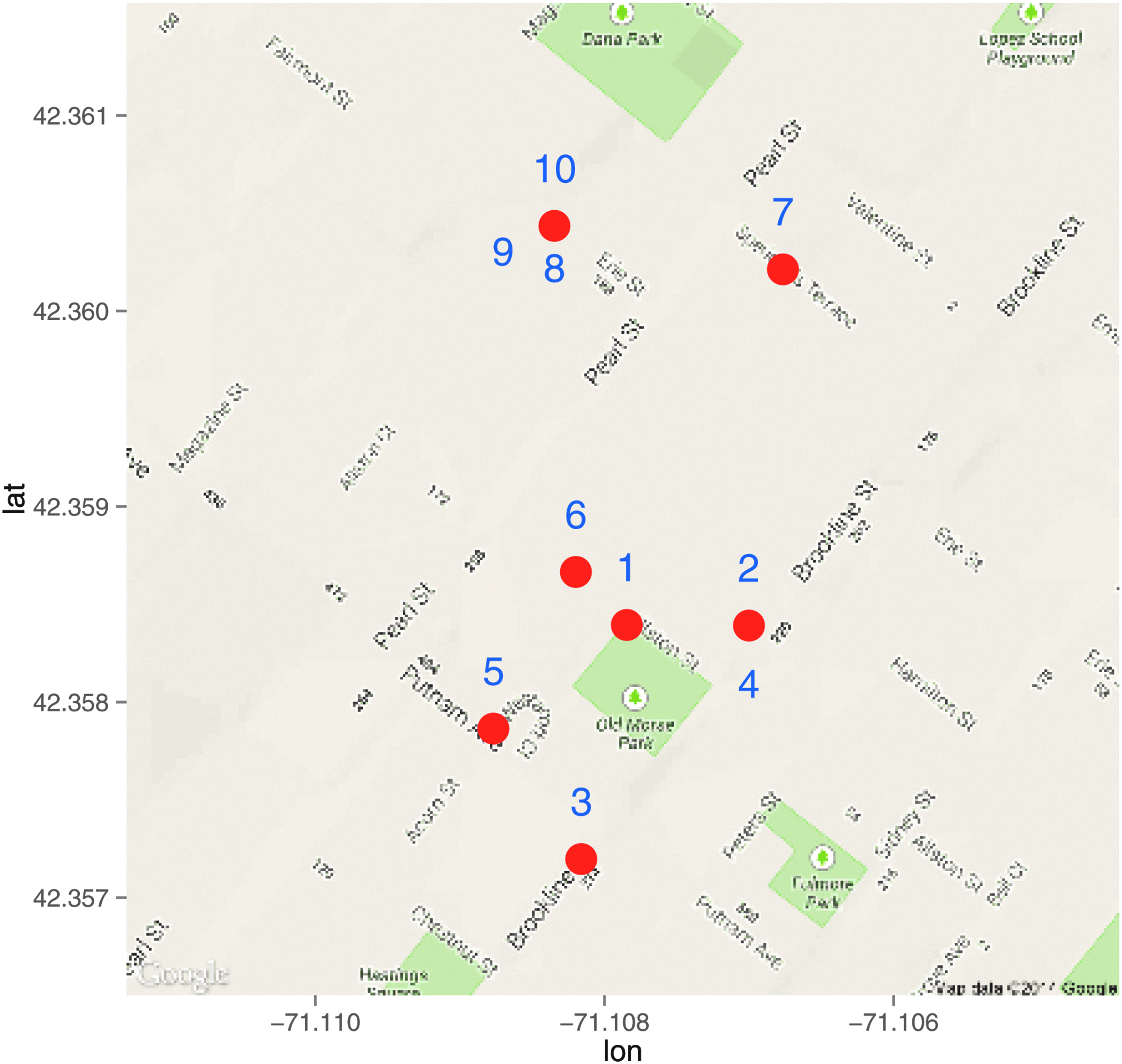
The locations of crimes in the first series.
Example 1 of a Serieslike Pattern with d=6
F, female; M, male.
From the (pattern-general) similarity graph, we isolated the subgraph containing the 10 crimes, which is diagrammed in Figure 8. Crimes 1 to 5 are well connected as a subset, and crimes 6 to 10 are well connected as another subset. From only the similarity graph, the two subsets do not seem very related except for a single edge between crimes {5, 6} connecting them; however, this is only the pattern-general part of the story.
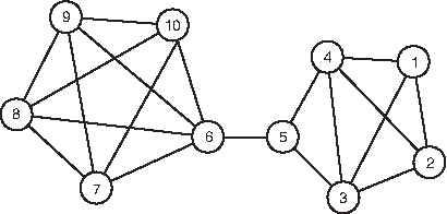
Similarity graph for the first crime series.
We used the integer linear program (12) to discover cores of size 3 with at least 6 defining features. Table 3 lists the cores and their defining features in this series, where a check mark means the feature is a defining feature and a circle means it is not. These cores show how the crimes are similar to each other in a pattern-specific way. The next step is merging the cores. The defining feature set Π(G) was chosen to include six features, which are geographic location, days apart, location of entry, the ransacked indicator, time of day, and day of the week. One of the cores, core 16 in Table 3, which was not included as geographic location is not a defining feature for that core, and the rest of the cores were merged. (The same set of crimes is in the merged pattern regardless of whether core 16 was used for the merge.)
Cores and Their Defining Features for Example 1
As these data were reconsidered by crime analysts, we found out that when these crimes were analyzed back in 2006–2007, they were viewed as two unrelated patterns, one at the end of 2006, crimes 1 to 5, and one at the beginning of 2007, crimes 6 to 10. The connection between these two subsets of crime is very subtle, and there is over a month gap between the two patterns, so it did not occur to the crime analysts to link them. Their intuition agrees completely with the similarity graph, as the two subsets are weakly connected only by one edge; however, recall that this only describes the pattern-general similarity–what one would expect from generic pattern without considering a specific M.O. On examination of the cores, not only are they correlated in six features, but five of the cores (core indices 11, 12, 14, 15, 16) contain crimes from both of the subsets, which is strong evidence that the two subsets should be merged together. It is particularly interesting that the core consisting of crimes 5, 6, and 7 spanned the two subsets, where these crimes share the unusual feature that residents were present during the break-in.
We wondered why the offenders changed their M.O. to move a few blocks north since they committed crimes 1–6 in the same area. What may have happened is that the criminals left near the end of December (just before the holidays), and returned in February to commit housebreak number 6 in the same area as 1–5; however, they were witnessed committing crime 6 (suspect information in crime 6 reads “3 males”). This may have spooked the offenders, causing them to alter their M.O. by moving north to commit crimes 7–10. Analysts now believe that these two series were actually a single series, and that the suspect information from crime 6 can be carried through to all the crimes in the discovered series.
This is a good example to show how crime patterns can be composed of cores and exhibit similarity both in a pattern-general way and a pattern-specific way. It shows how we can use both aspects to mine patterns. This is a pattern that would be very difficult for a crime analyst to find: the M.O. changes over time, there was a long break in the middle of the series, and there was nothing deterministic (e.g., fingerprints) linking these crimes.
Case study 2
Table 4 and Figure 9 show a more typical pattern in 2007 discovered by our method. The crimes were committed on two dates in late January 2007, most of them in the same building. According to the Cambridge police, they arrested a suspect while he was committing the last crime in the series and confirmed that he did commit crimes 2–7. Note that the record for the fourth crime records the means of entry as “key.” This is based only on the claim of a witness that the offender possesses a master key. If the offender did possess a master key to the apartments in the building, it would explain why the means of entry was unknown for other crimes in the series—the means of entry would thus have been very difficult to determine for earlier crimes where residents were not present.
The locations of crimes in the second series.
Data from the Second Crime Series
Case study 3
Our method has also been used to help ensure the fidelity of the historical database of past crimes. We ran our method using data collected prior to 2006 to see whether we would be able to make discoveries.
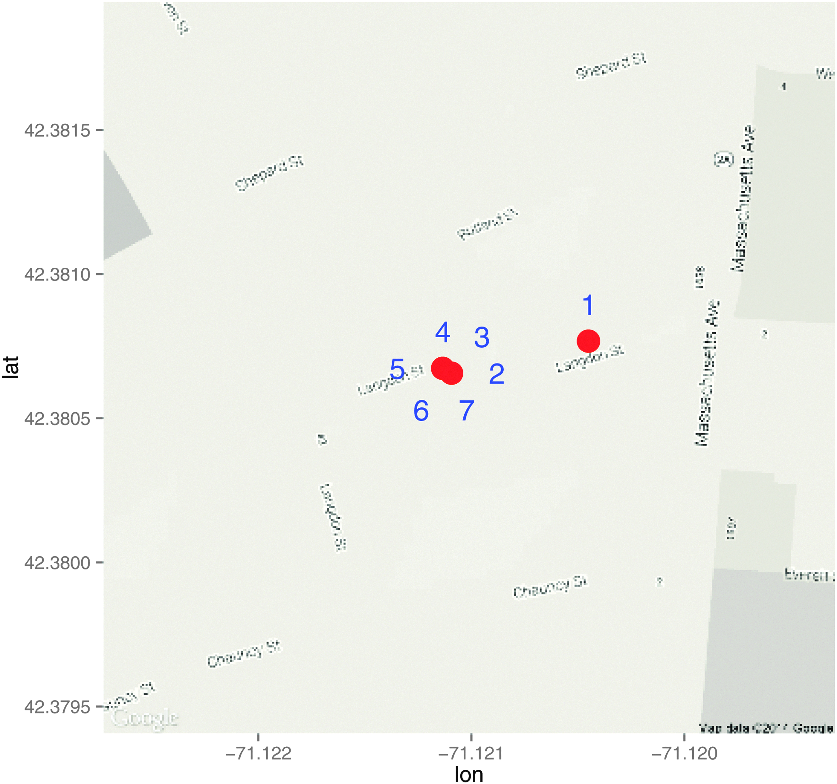
Table 5 shows details from crimes within a 2005 pattern, discovered by both the police and our algorithm. Our algorithm and the crime analysts agreed on six out of the eight crimes in the series, but disagreed on two crimes: crime 3 and crime 4. The crime analysts identified these crimes as part of the pattern, but our algorithms did not identify these crimes as being part of the pattern. Our algorithm provides reasons why these crimes should be excluded from the pattern: They are not close to other crimes in the pattern-general sense and are not connected to the other crimes in the series within the similarity graph, as depicted in Figure 10. Neither of the crimes are contained in any cores, as shown in Table 6. In particular, the map in Figure 11 shows that these two crimes are geographically far away from the other crimes. Since geographic closeness has a large contribution to pattern-general similarity, crimes 3 and 4 are already not likely to be part of the same series. Besides that, we also notice that other aspects of crimes 3 and 4 differ from the rest of the pattern (see Table 5). In crime 4, the means of entry is by key, which is different from that of other crimes where entries were forced or pried. According to police narratives, the fourth crime had a 91-year-old victim, who reported that $35 was stolen from her purse by someone who used a key to enter the apartment; this indicates the crime was not part of the series, and further indicates the possibility that this crime never actually occurred. In crime 3, the apartment was ransacked while none of the other locations were. The narrative for the third crime is very generic: someone broke in through the living room window, stole jewelry and loose change, and exited through the front door. It is not clear that this crime possesses any distinguishing characteristics to identify it as being part of the series.
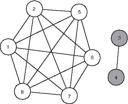
Similarity graph for the third crime series.
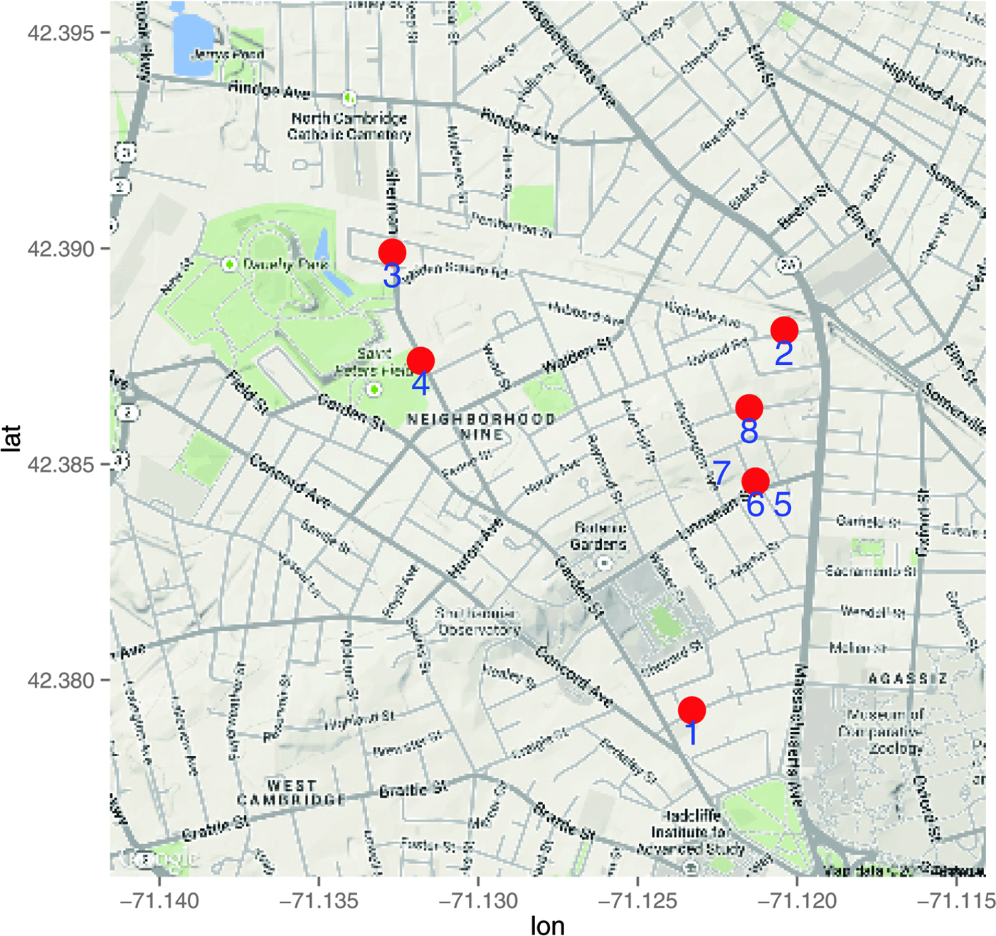
The locations of crimes in the third series.
The Third Serieslike Pattern with d=5
Cores and Their Defining Features for Example 4
When examining the crime series retrospectively, the police agreed that crimes 3 and 4 likely should be excluded from the pattern (note that this pattern has not been officially verified through an arrest).
Conclusions
The problem of detecting crime series is both subtle and difficult. In cases where crime series detection is trivial, meaning that there is identifiable information about the criminal (e.g., fingerprints or DNA) then sophisticated modeling techniques are not needed—the solution is direct in those cases. The more subtle cases where crime series might otherwise become hidden in a sea of data are where data mining methods can shine. Our automated series detection methods are able to detect crime patterns within big data sets where a human could not. Detecting patterns among crime data is critical to effective policing. When a pattern is identified, police can implement effective strategies to prevent future crimes, solve past crimes, identify and capture offenders, and ensure offenders are investigated and prosecuted fully for the crimes for which they are responsible. We envision that methods such as ours could be used very broadly for crime series detection, and would be particularly useful across regions or districts, where human crime analysts would fail to be able to manually handle vast amounts of data from several different regions or data sources in order to detect patterns.
Footnotes
Acknowledgment
This work was supported by a grant from MIT Lincoln Laboratories.
Author Disclosure Statement
No competing financial interests exist.
Cite this article as: Wang T, Rudin C, Wagner D, Sevieri R (2015) Finding patterns with a rotten core: data mining for crime series with cores. Big Data 3:1, 3–21, DOI: 10.1089/big.2014.0021.