
Abstract
Abstract
Our goal is to design a prediction and decision system for real-time use during a professional car race. In designing a knowledge discovery process for racing, we faced several challenges that were overcome only when domain knowledge of racing was carefully infused within statistical modeling techniques. In this article, we describe how we leveraged expert knowledge of the domain to produce a real-time decision system for tire changes within a race. Our forecasts have the potential to impact how racing teams can optimize strategy by making tire-change decisions to benefit their rank position. Our work significantly expands previous research on sports analytics, as it is the only work on analytical methods for within-race prediction and decision making for professional car racing.
Introduction
C
There are many other sports in which key strategic decisions are made without the help of in-game analytical tools. Even in sports like baseball and basketball, where there has been a lot of work on analytics, analyses are typically done at the season level, prior to the start of the game. This is very different than our work because, in racing, the actual conditions of the race are potentially very useful for predicting the outcomes, beyond what one can obtain using season-level statistics.
This work started with the hypothesis that a data-driven prediction engine operating in real time may be able to assist team captains in making these critical tire-change decisions. As no such prediction software or methodology previously existed, it was unclear how the data could be leveraged to produce an accurate prediction model; there was no previous knowledge discovery system for working with data from professional stock car races or from any similar enough sport. Further, the predictions need to be made at the finest granularity available for racing data—at the level of individual laps—which is the most detailed race-level data made available to teams by  (at least through 2012). While constructing a knowledge discovery system for these data, we faced considerable challenges in how to process and define the prediction model. In handling racing data, it is easy for a bad mathematical definition to lead to a conclusion that a particular feature is not important for prediction, and it is easy for Simpson's paradox to appear, indicating (for instance) that tire-change decisions do not impact race position. In the end, we were able to obtain high-quality results only when domain expert knowledge about racing was carefully infused into all of the mathematically defined features and evaluation metrics used in the prediction engine.
“This work started with the hypothesis that a data-driven prediction engine operating in real time may be able to assist team captains in making these critical tire-change decisions.”
We consider the entire cycle of the knowledge discovery process: exploratory analysis, feature generation, building a model, data mining, and decision making for within-race strategies. Mining the raw data requires many domain-specific considerations in order to construct meaningful statistics. Model building requires careful assumptions about the observed data and molding the problem into a tractable learning formulation. Based on the model outputs, decision making requires an understanding of the horizon and time scale where it is most meaningful to make a decision and characterize its risk–reward tradeoff. In the sports-prediction and decision-making studies of the past, these components have been examined mainly in isolation. Our study can be abstracted to a framework that is both unified and tractable, allowing the possibility of system-optimal solutions in a practical amount of time (instantaneously) for professional racing and other sports.
The statistical hypotheses we address will be derived from the following questions:
Q1. Can we predict the change in rank position of a racer over the next portion of the race, based on the racers' recent histories? Q2. Can we optimize within-race tire change and refueling strategies based on the predicted future performance of a racer? Q3. Can we gain insight from past races that can assist the team in a future race?
Considering question Q1, the design of in-race data-driven strategies critically relies on our ability to forecast the performance of the racer based on his and his neighbors' recent race history, the state of the race up to that point, and any decisions he can potentially make (zero tires, two tires, or four tires). The racer's recent history can include the number of other racers he overtook, the racer's speed, rank position, and the age of each of his tires. Another valuable outcome of answering Q1 is being able to forecast the finishing rank as early as possible within the race. This is conventionally forecasted using season-level data before the race even starts.
To determine strategy, we need to know beforehand what the impact of a racer's tire change will be on his rank position and deceleration. It is possible for a racer to rapidly gain rank position by changing zero or two tires during a pit stop, but this action can penalize his ability to maintain this rank position throughout the next portion of the race. This effect can be highly complex and dependent not just on the racer but on the tire-change decisions of other racers, the track itself, the track temperature and weather, and the type of tires used for the race. Yet, being able to forecast the impact of a tire-change decision can assist with critical elements of racing strategies; in other words, answering Q1 can lead to an answer to Q2. For instance, a reasonable myopic strategy is as follows: If we predict that a two-tire change is likely to lead to a loss in track position compared to a four-tire change, the team captain could make a decision to change four tires. Answering Q2 is important because strategies may have a large impact on the racer's success when all his peers are almost equally skilled and the cars have very comparable speeds.
Besides the goals of real-time prediction and decision making, a knowledge discovery framework for racing can help provide specific insights into racing strategy (Q3). It can be a valuable tool for reasoning about how different actions in the past have impacted the subsequent rank positions of the racers. For instance, does the value of the prediction depend on the forecast horizon? Does the variability of laps raced between tire changes have an effect on ranks? We would like to know answers to such questions because they can lead to better predictions and insights for future races.
The following section provides related work. In the third section, we describe some of the complexities we encountered in the knowledge discovery process in our setting. We also describe some experimental shortcomings that restrict the predictions and inferences we can make. In the fourth section, we define the prediction problem and describe the key hypotheses about our data that guide our construction of features for predicting change in rank position. A straightforward myopic decision-making step is proposed to address Q2. Prediction results are provided in the fifth section, answering Q1. Some insights from the knowledge discovery process are mentioned in the last section in an attempt to answer Q3.
Related Works
Work on knowledge discovery systems in different domains have highlighted some of the important challenges that we also face in this work (see, for instance, Refs.2–9 ) In particular, these works have highlighted the importance of designing knowledge discovery systems around the unique aspects of a domain. These works also emphasize the key choice of proper evaluation metrics and being able to provide insight that goes beyond prediction accuracy and back to the important aspects of the domain. The choice of machine learning algorithm itself is not always a critical choice within a knowledge discovery system; in our data mining step, we found that several different algorithms have essentially similar performance.
There have been few recent attempts to use prediction models for in-game decision making in sports such as baseball,10,11 basketball, 12 and cricket.13,14 This is contrasted with season-level statistical modeling, which is well researched in the literature because of their applicability, in particular, to sports betting and fantasy sports in addition to helping the teams improve their competencies (see Ref. 15 for a brief overview). Note that for professional racing, season-level research has been sparse (see, for instance, Refs.16–19 ) and our work is the first to explore in-race predictive modeling.
For baseball, Ganeshapillai and Guttag 10 developed a prediction model to decide when to change the starting pitcher as the game progresses. Similar to our workflow, they proposed several features from historical data and the current game's history to predict a pitcher's performance. At a given point in the game, they forecast the future performance of the pitcher, compare it to a predefined threshold, and make a binary myopic decision whether the pitcher should continue or not. A related work 11 looks at predicting the type of pitch that will be thrown by a pitcher given the current state of the game and historical data about the teams playing.
In basketball, Bhandari et al. 12 developed a knowledge discovery and data mining framework for the National Basketball Association (NBA) with the aim of discovering interesting patterns in basketball games. This and related (often proprietary) systems have been in operation with many basketball teams over the past decade. Such solutions are tailored for offline use and do not address in-game prediction and decision making as we do. There has also been some recent work 20 exploring in-game decision making as a function of time remaining in the game without building any prediction models.
A key difference between predictive modeling for professional racing compared to that in basketball (and baseball) is the nature of the evolution of the game. In racing, the race history cannot be easily segmented into “plays.” At each point in time of a race, the entire history of the race determines the racer's current rank position. On the other hand, in basketball, the game is restarted at the beginning of each play and the team's current state does not heavily depend on their state before the restart. One can reasonably approximate a basketball game to be a sequence of independent plays and even model them as independent observations drawn from a distribution. These long-standing correlations of decisions within the race makes racing inherently much more difficult to model.
“A key difference between predictive modeling for professional racing compared to that in basketball (and baseball) is the nature of the evolution of the game.”
In cricket, Bailey and Clarke
13
and Sankaranarayanan et al.
14
explored machine learning methods to predict the future states of the game given features related to the current state of the game and the features of the two teams competing. They consider both season-level data and the data collected within the game to predict future scores. Although both these works are closer to what we do, there are a couple of key differences: (a) these works involve a much lower dimensional prediction problem (about 15 features in Sankaranarayanan et al.
14
) compared to ours (>100, see the Prediction Framework section), and (b) professional racing involves many more strategic agents (for , about 40 racers race) compared to cricket (two teams, which is is also the case for basketball and baseball). We believe having a high number of strategic agents can have significant impact on predictability and makes the knowledge discovery process more critical compared to two-team games.
Another key feature of our work is that we explore the knowledge discovery pipeline extensively compared to the previous works. This is partially because for basketball, baseball, and even cricket, there has been significant prior academic research output compared to professional racing. In this work, we critically examine many details and characteristics of in the section Data and Observations. For instance, we observe Simpson's paradox-like phenomena between two explanatory variables (slope of lap times and number of tires changed). Our exploration of data can help future work on racing focus more on statistical modeling and prediction as in baseball and basketball.
The need for predictions at the finest granularity of racing is two-fold: 1) Previous studies on racing, like those using only race-level and season-level statistics, may be too coarse to be beneficial within the middle of a race. For example, we believe that statistics computed during the race, for instance, the state of the race after 100 laps, often reveal more about the outcomes of the current race than the predictions made by the previous studies. Season-level and multi-year studies are also susceptible to changes in the rules or other changes to the sporting event. For example, for , rules have changed multiple times, the latest ones being in 2008 and 2011. This further reduces the effectiveness of race-level statistics for aiding racing strategy. 2) By calculating within-race predictions dynamically as the race evolves, we can better quantify the contribution of real-time observations toward predicting outcomes in each portion of the race.
Finally, we note that the approach we take to building a knowledge discovery framework and decision-making system for professional racing can be applied to other racing sports with similar structural characteristics, including MotoGP (see also Ref.
21
), Formula 1, IndyCAR, various other types of races within , and also bicycle races and marathons.*
Data and Observations
We define some of the race-specific terms used in the article:
• Lap: One full trip around the race track. • Lap time: The time for a racer to finish one lap. • Rank position: The position of the racer at the end of a lap. If the position is 1, the racer is leading the race. • Pit stop: The event in the race when a racer stops racing and enters the pit (area where cars are serviced) with the intention of changing tires or refueling. • Caution lap, or yellow lap: A lap is called a caution lap
†
when the racers are not actively racing, have slowed down and are following a “safety car.” Caution flags (yellow flags) are displayed due to a hazard on the track (crash, tire burst, etc). In our racing data set, caution flags are a random influence that substantially affect race dynamics. • Green lap: Laps that are not in caution are called green laps. • Warm-up period: After a racer's pit stop or after the end of a caution, the warm-up period includes green laps in which the lap times are decreasing successively as the car gains speed. • Epoch: The green laps after the warm-up period–until the next pit stop or caution lap–constitute an epoch. • Outing: The green laps in the warm-up period and epoch together form an outing for the racer.
In our study, we use race data constituting 119,178 lap times and 119,178 rank position observations from 2,932 total outings, including each racer's lap times and rank positions for each one of the 5,352 laps within our data set. We also have caution lap and pit stop information (time and number of tires changed) for each racer. (Some races had unusual race characteristics, for instance, some were road courses and some had insufficient or missing tire change information; thus, these were not used in our study.) Races comprising this data set are listed in Table 1. The numbers of laps in the 17 races we examine range between 160 and 500 laps. The total number of pit stops per race varies between 170 and 373, and the average number of pit stops per racer varies from 4 to 8.9. The number of cautions varies between 3 and 14.
Complexities of racing
To give a sense of the difficulty in modeling with racing data, we next discuss general characteristics of racing and how nonlinear interactions between measurements and other issues pose difficulties in modeling and decision making. Several of these observations have not (as far as we know) been previously quantified, in particular, the “fresh air” effect and the Simpson's paradox effect from tire-change decisions discussed below.
Tire-change decisions
As we discussed, this is a major strategic decision for each team. In isolation, a car with four fresh tires is generally faster than a car with only two fresh tires; however, it is not that simple during a race. The speed of racers is heavily dependent on more than just tire freshness; as we will discuss, rank position and the ability to overtake other racers play important roles in determining speed. A two-tire change may or may not be an overall advantage depending on whether the racer is also able to maintain their rank position.
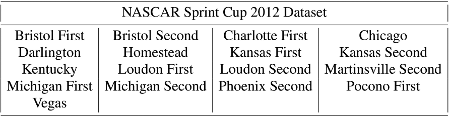
Choosing a two-tire change saves a racing team about 6 seconds on average over a four-tire change, though there is a high variance in pit times. Pit lanes have speed limits that dictate the minimum pit road time, and the racer has to slow down while stopping at his designated stop, make turns into and out of his stop, and avoid other racers executing pit stops around him. These elements and the actual performance of the pit crew in servicing the car determine the pit stop times. Figure 1 shows the histogram of pit times. One can see three peaks (around 4 seconds, 7 seconds, and 14 seconds) and a peak at 0 seconds. The 0-second pit times are due to penalties among other causes (including missing data defaulting to 0). The other three peaks are due to the decision to replace zero, two, and four tires respectively. A zero-tire pit stop is for refueling only.
Histogram of pit times taken by various racers in our data set.
Saw tooth profile of lap times
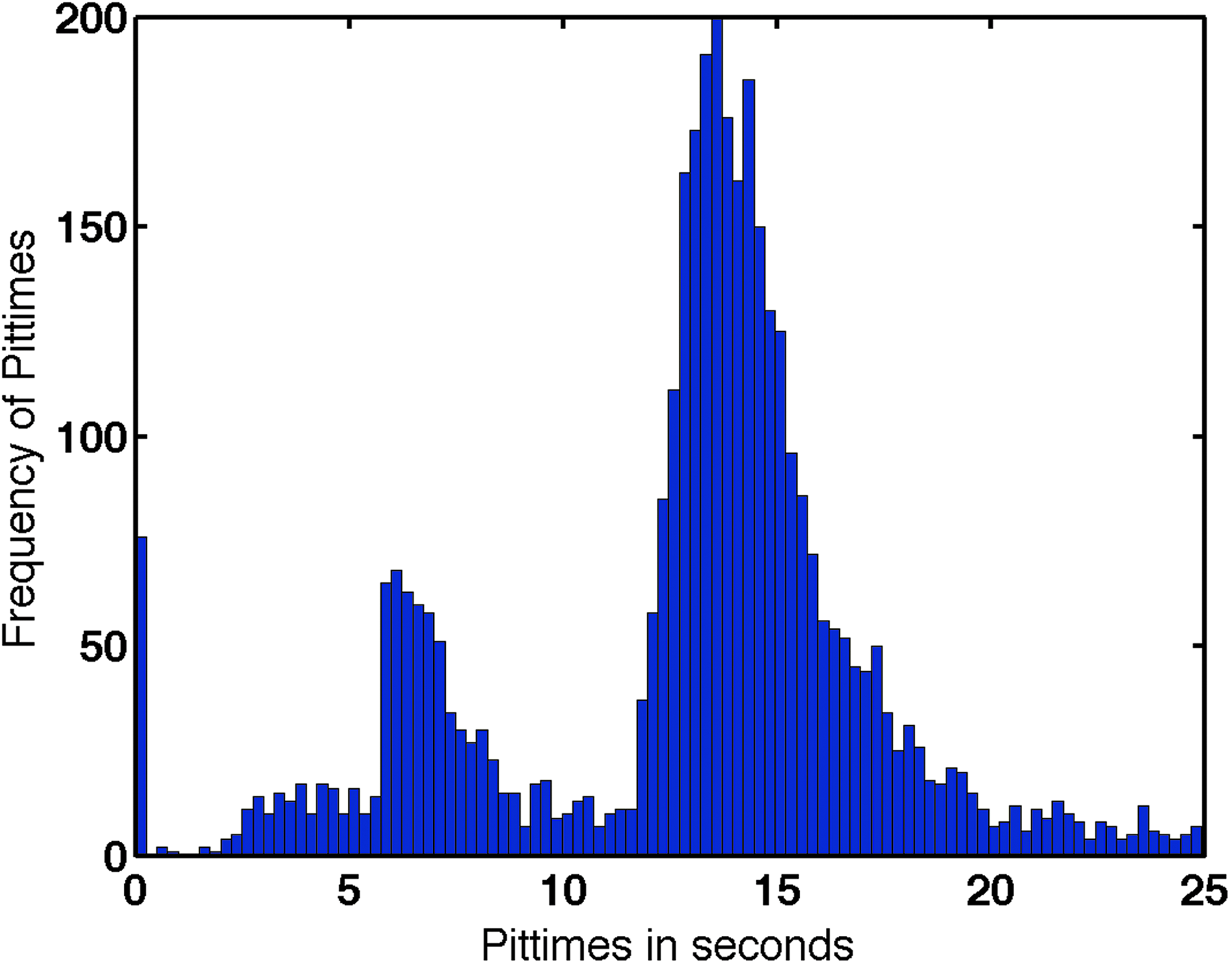
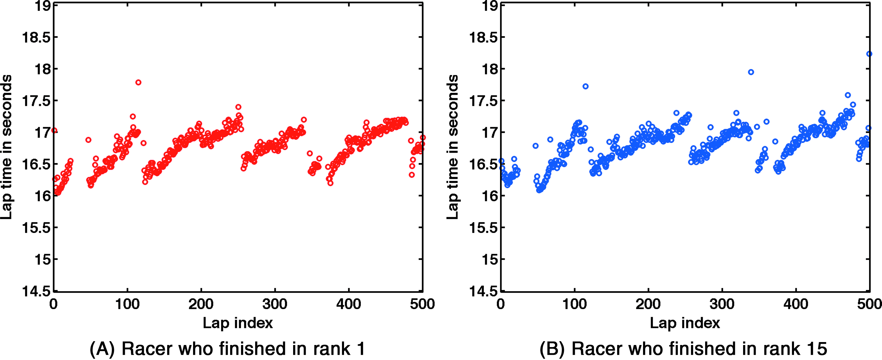
Examples of the lap-time time series for typical racers in our dataset is shown in Figure 2. Lap times increase (the car gets slower) as the tires wear down over the course of an outing. Toward the end of an outing, one can also see that the lap times sometimes flatten out; the lap times deteriorate at a slower pace later in the outing. We use the slope (estimated rate of change in seconds per lap) of these lap times over the course of an outing to measure tire wear. See Figure 3 for an example of how slopes are computed.
Sawtooth profile of typical racers in a race.
Plot of lap times and linear fits for a 15th ranked racer in a race. Slopes are computed by fitting a line through the lap times in an outing using simple linear regression.
The “fresh air” effect, which is a nonlinear interaction between lap time and rank position
In general, lap times are lower (better) for racers near the front of the pack. This is illustrated in Figure 4 for three typical laps in three different races. Remarkably, a linearly increasing trend is plainly visible between lap time and rank position in each figure. That is, the lap speeds of racers at the front of the pack can be substantially faster than those in the middle of the pack, which can be substantially faster than racers at the back of the pack.
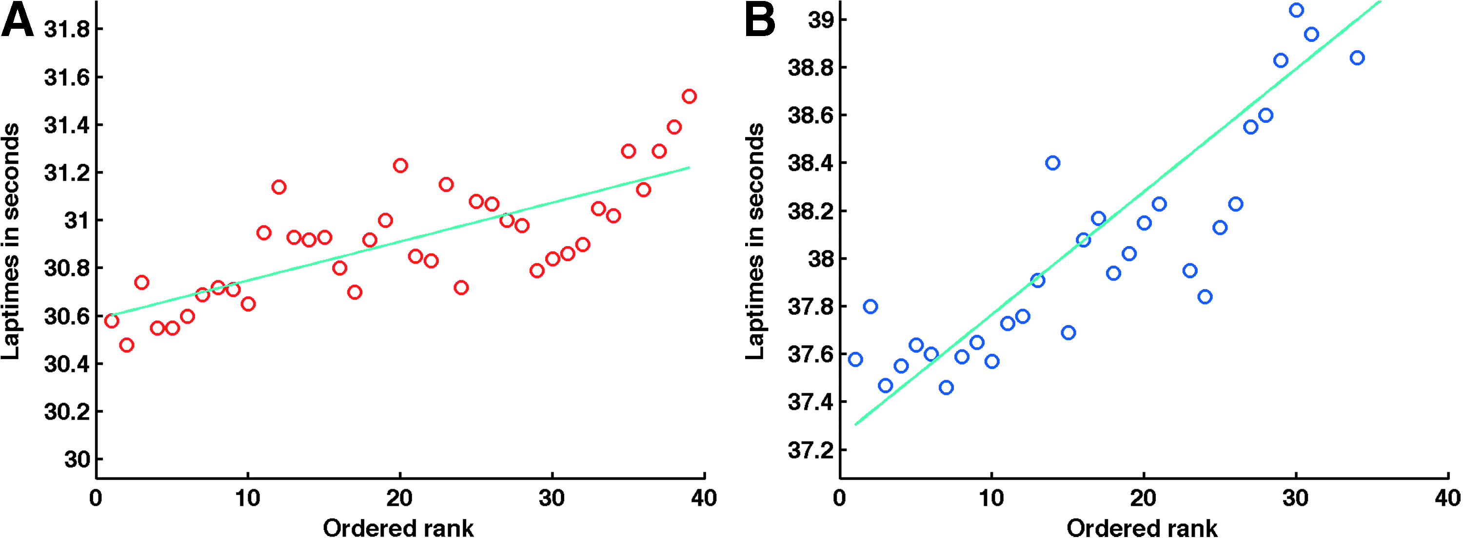
Fresh air effect: ordered lap times of the racers at lap 50, sorted by rank position, for two separate races. Each dot represents a racer's lap time. There are about 40 racers in each plot.
Because racers near the front of the pack tend to go faster, their tires wear out more quickly. In fact, we observe that the slope of lap times over an outing increases more quickly for cars at the front of the pack. This is shown in Figure 5. Actually this effect is highly nonlinear: The cars in the front of the pack and the back of the pack tend to have higher slopes, and the cars in the middle tend to have lower slopes. The effect is fit nicely by a degree-2 polynomial, as shown in Figure 5.
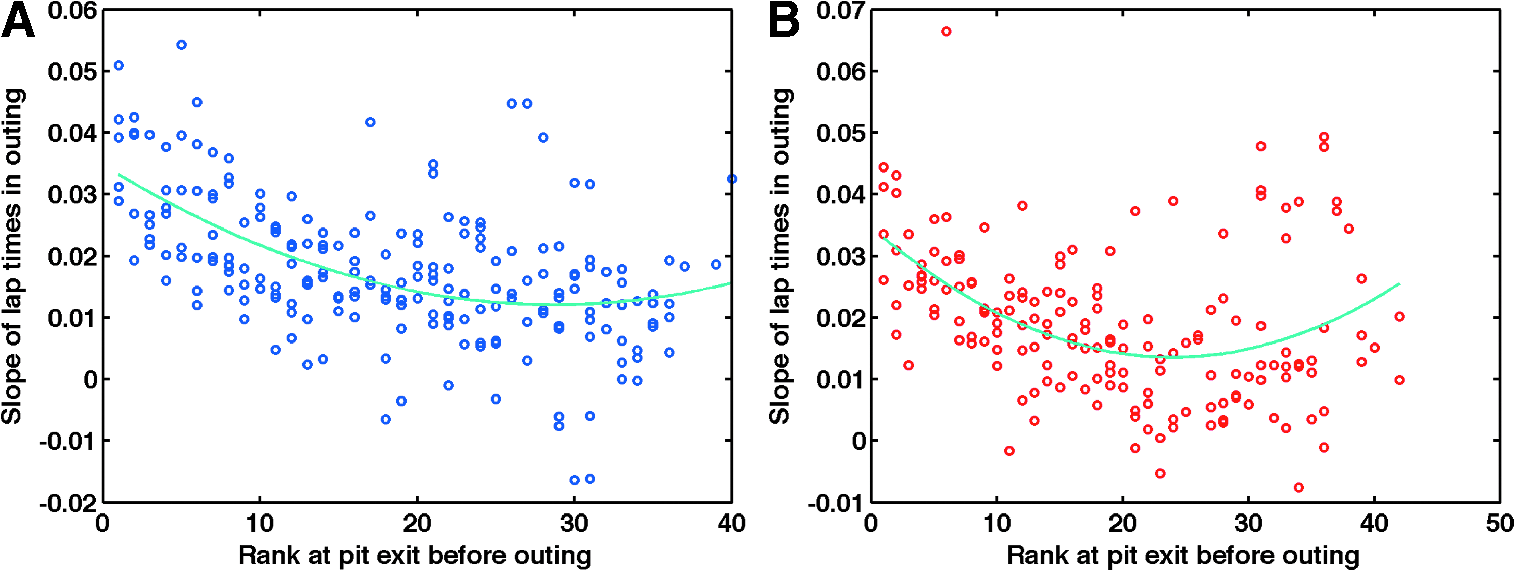
Slopes of lap times within an outing versus initial rank in the outing, for two separate races. Each dot represents a racer's outing within a race. In a typical race, each racer has multiple outings; thus, there are multiple dots for each of the ∼40 racers in each race.
Simpson's paradox ‡ for the number of tires changed and the slope
Consider the leftmost subplot of Figure 6, which shows the distribution of slopes for two tire changes and the distribution of slopes for four tire changes during a race. It is clear that in this race, cars that took two tires had much faster wear (higher slopes) than cars that took four tires. This seems to indicate that older tires tend to wear faster for this race, and thus if the epochs are sufficiently long, it would generally be strategic to take four tires. However, this is a severely incomplete picture. In fact, rank position is a lurking variable, in the sense of Simpson's paradox, and has the following effects:
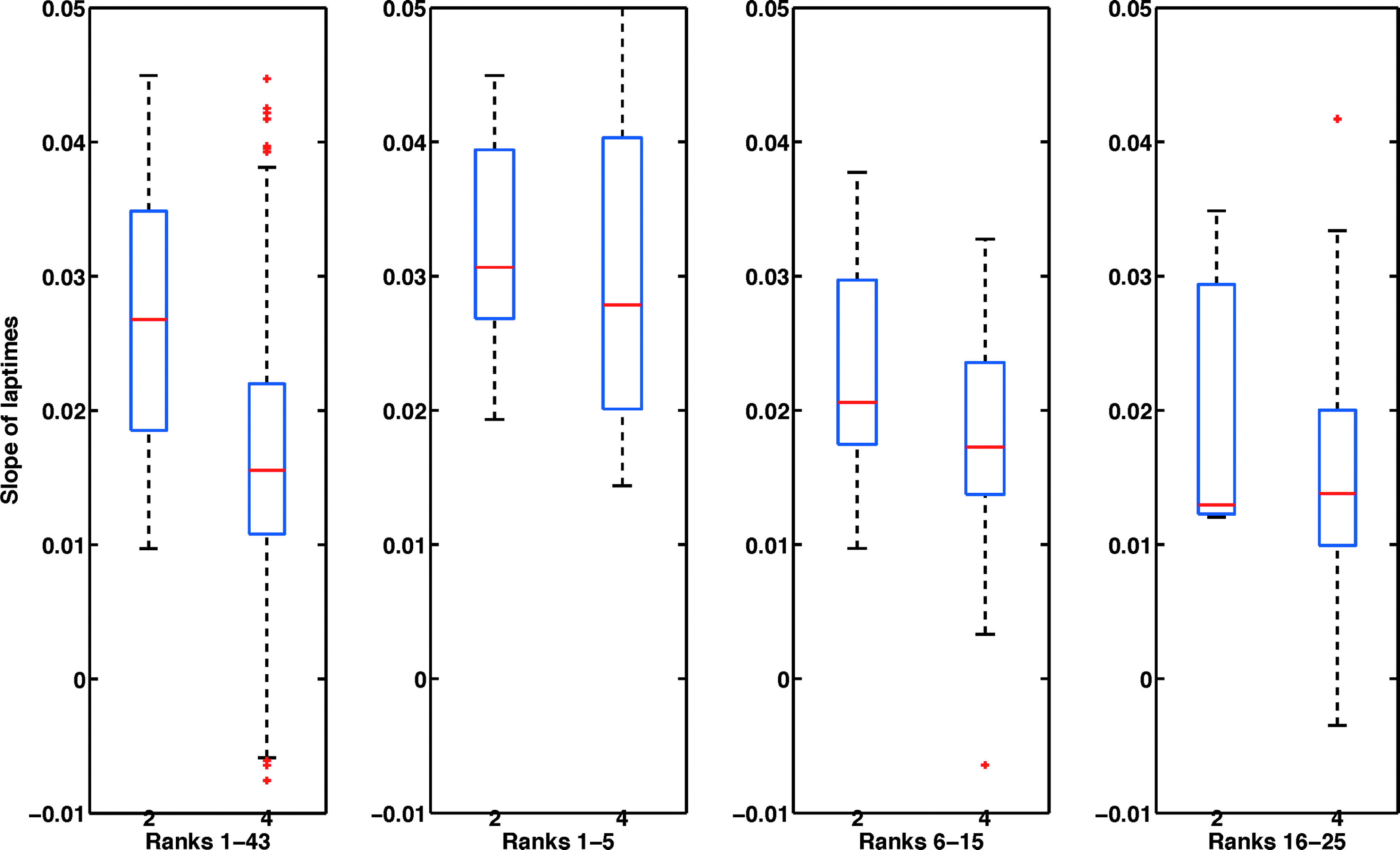
On the left, we include slopes for all ranks on a single boxplot. The right three boxplots again show the distribution of slopes, but separated by rank position. Rank position can be considered the lurking variable for Simpson's paradox, as the right three boxplots refute the hypothesis from the left boxplot—namely, that the slopes for two-tire changes are substantially larger than the slopes for four-tire changes. In these boxplots, there were 26 two-tire changes and 176 four-tire changes. These data are from a track in the midwest of the United States.
(a) Because only cars that have generally better rank positions take two tires, their slopes are also higher (as we showed in Fig. 5). In fact, for racers in ranks 26–43, there are no instances of two tire changes compared to 49 instances of four tire changes. This results in a lower median slope for four tire changes, as shown in the leftmost subplot in Figure 6.
(b) If we break down our data according to rank positions 1–5, 6–15, and 16–25 as shown in the three subplots to the right in Figure 6, we see that the median slope values across ranks are actually very similar for two tire changes and for four tire changes, in seeming contradiction with the leftmost boxplot.
Thus, conclusions drawn from simply looking at slopes for two tire changes and slopes for four tire changes, as in the left of Figure 6, would be misleading. Note that the impact of the two- or four-tire decision depends on many factors besides rank position. When the distribution of slopes are similar as in the box plots for rank positions 1–5, two-tire changes would be strategic since the racer could gain rank position without any predictable change in the rate of tire wear.
Race dynamics around a green lap pit stop are different from those after a caution lap pit stop
Racers may choose to pit during a green lap to refresh tires and/or refuel. Not all cars take green lap pit stops around the same time, which causes a high variance in rank positions around the laps when these pit stops occur. For instance, a 20th-rank position racer, who has been in the same position through the outing, can become a first-rank position racer temporarily if the 19 racers in front of him pit while he does not. Usually, he will then pit in the succeeding laps. While the other cars are in the pit and he is not, his first-rank position is artificial. Also, in this case, his pit entry rank position would be recorded as 1. Thus, the green lap pit stops can be very problematic for our analysis, as rank position is not completely meaningful when other racers are in the pits. Caution lap pit stops, on the other hand, are less susceptible to high variability. In the case of outings preceded by green lap pit stops, the racers are more spread out on the track than in the outings preceded by caution lap pit stops (which are similar to a race restart).
Game theoretic aspects (neighborhood interaction)
Neighboring racers impact each other because of shared track space. This is a key difference from other racing sports like athletic short distance track events or indoor swimming where there is minimal neighborhood influence since each player has his own assigned lane.
Data issues
Besides the inherent complexities of racing discussed above, there are some natural challenges that arise when making decisions based on historical data. In , the decision to replace two tires versus four tires is one such case, particularly due to the data problems of control, imbalance, and noise described below.
No controlled experiments
Recall that our objective was to make informed decisions (two tire or four tire) based on race history. Unfortunately, we cannot perform randomized controlled trials in order to measure the effect of a decision; we are limited by what we can do with the historical data. One way to partially handle this shortcoming is to pick “similar” racers who differ only in their tire decisions and verify whether there is any difference in the causal effect of the decision. Again this is unsatisfactory, as controlling for all other variables in the system is very difficult.
“Unfortunately, we cannot perform randomized controlled trials in order to measure the effect of a decision; we are limited by what we can do with the historical data.”
Imbalance
There are far more four-tire pit stops than two-tire pit stops. This makes it difficult to quantify the effect of the number of tires on the performance of the racer. Figure 7a shows the number of two-and four-tire pit stops in each race of our data set. In addition, almost all practice before a race is based on four-tire changes with the intention of tuning the settings of the car. During practice runs, the total number of tires and total laps that can be run are budgeted as well.
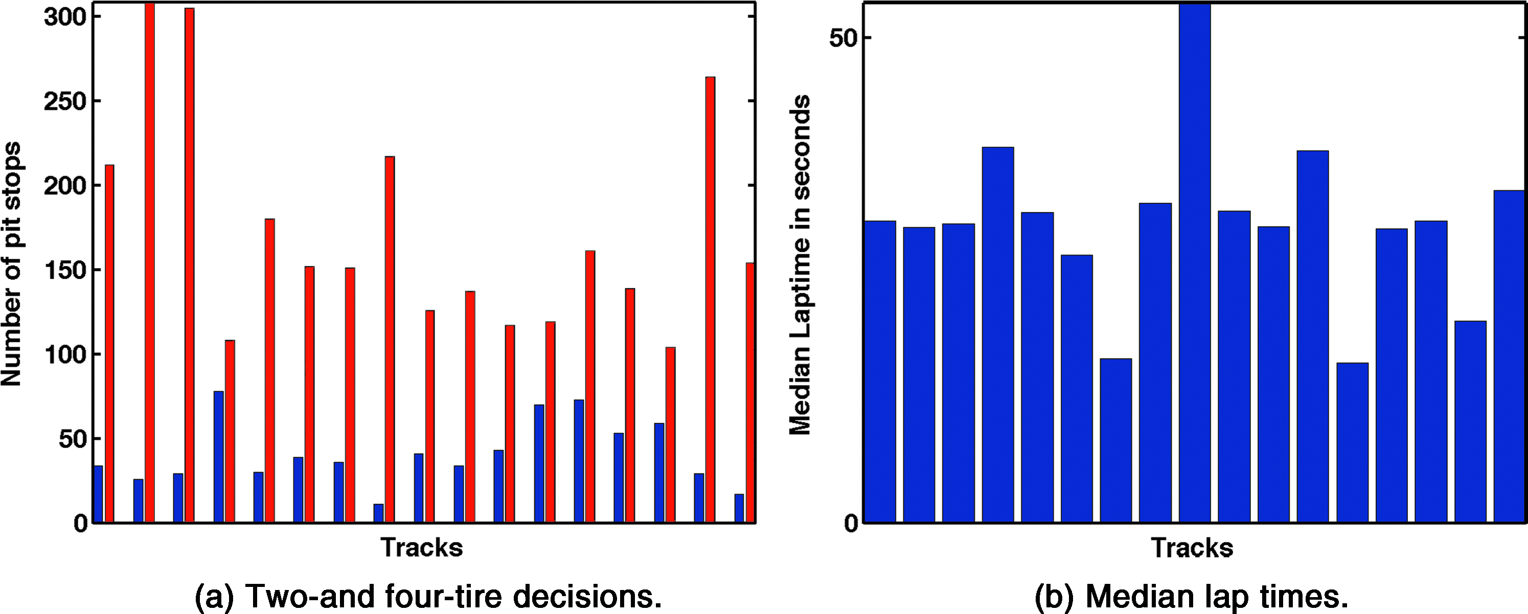
Bar plot of two-and four-tire decisions per race for our data set is plotted in
Races are different
We would like to be able to generalize knowledge (or borrow strength) across races. However, races can be fundamentally different, prohibiting a straightforward merging of observations across races. The number of laps in the race, the length of the tracks, and their physical characteristics (e.g., banking characteristics) can be very different, which all heavily affect lap times. For instance, Figure 7b shows the median lap times of races we analyze, where the median is taken over all racers and all laps; these heavily vary from race to race. In general, statistics of pit information and lap time information are not race invariant and cannot be directly compared across races.
Noise
“Irregularities” in racing occur very regularly, such as having accidents (hitting the wall, spinning out of control), running completely out of gas, experiencing mechanical failures, and incurring race penalties. These irregularities can affect the quality of our predictions if they are not carefully filtered out. Another aspect that adds to the noise is out-of-sequence pit stops, where a racer takes a pit stop at a different time than the majority, altering the rank positions of others temporarily. Race rules such as “free pass” § and strategies such as staying out to lead a lap to earn a point also make our observations noisy.
Prediction Framework
Keeping in mind the complexities of racing and the data issues discussed above, we now discuss our framework for real-time prediction and strategy in racing.
The prediction problem
Based on the Complexities of Racing section we made the following choices about the time scale of learning and the dependent variable.
We chose to forecast the decision-to-decision loss in rank position for each racer, for each decision during the race. This is the change in rank from a car's pit entry to the end of its next outing when it enters the pit again. If we are able to predict this quantity, taking into account the racer's current state, his race history, and previous decisions, this will tell us whether the racer's current strategy may give him an advantage between the current decision time and the next one. Note that since a majority of outings end due to cautions, the racer's strategy does not generally determine the end of the outing. The prediction interval includes a pit stop and the outing following it for a given racer. Our system makes a prediction before each prediction interval. Because of this choice of model formulation, our prediction problem becomes a supervised learning problem, for which we can use a range of supervised learning techniques.
We chose to model the change in rank position and not other functions of the outing (for instance, slope of lap times) because improvement in rank is really the goal of the team rather than improvements in, for instance, lap time. One might be tempted instead to model the direct results of a tire-change decision such as lap times, or equivalently, the slopes. However, slopes of lap times, though indicative of a racer's performance, are not a direct metric of success at the finish of the race. Also, as we discussed earlier, lap time measurements are heavily tied to rank position (see the Complexities of Racing section). Predicting rank position can still be complicated since, as we discussed earlier, it can depend on the timing of other racers' pit stops.
To build the prediction model, we use all race information from the current racer and his peers up to the pit entry lap index when our prediction interval starts. We also incorporate the team's planned action during the pit while learning from historical data. This naturally leads to the following myopic strategy: given a learned model, we can compute predictions for each planned action (zero, two, or four tires) and determine which action(s) might be strategic between now and the next time a decision is made.
Preprocessing
Our model needs to bypass the data issues discussed earlier, for instance, the artificial jumps in lap times caused by pit stops and cautions (the jumps in the sawtooth shape of the lap times discussed in the Complexities of Racing section). The key to this is to correctly create automated definitions of “outings,” “warm-up laps,” and “epochs.” We found that the prediction quality, interpretation of the prediction model, and potential value of predictions to the racers and the teams improved dramatically as a result of improving these model inputs, along with the other preprocessing steps discussed below. The definition we developed is fairly complicated and not fully discussed. For instance, our definitions are robust to events such as pit stops during green flags, which can cause a racer's rank position to be artificially inflated or deflated, impacting results. In the example we gave earlier, a racer with rank position 20 can come into the pit with rank position 1 if the 19 racers in front of him pit before him. To minimize the number of artificially inflated or deflated rank positions in our processed observations, we alter the pit entry lap indices appropriately. This way, the definition of the epoch has a smaller number of laps and aims to contain only the laps for which cars in front of the racer had not gone into the pit.
Key hypotheses
Based on exploratory analysis of lap time and rank position measurements, we believe the following key hypotheses impact our ability to predict change in rank. To our knowledge, these have not been published before.
“Rank momentum” leads to useful predictive factors
We compute a racer's “rank momentum” based on whether he is generally gaining or losing ranks. Simply, a racer that started at the back of the pack and continues to obtain better rank positions has a different trajectory than a racer that started out at the front of the pack and gradually moves toward the back. Rank momentum may help alleviate issues with the “fresh air” effect described in the Complexities of Racing section. Rank momentum terms rely on discrete derivatives of rank position time series. They capture information about racers relative to each other. This is different than the slope of lap times (“lap time momentum”), which considers the racers in absolute terms rather than relative to each other.
“Protection” and other neighborhood effects can lead to useful predictive factors
As we discussed, when a racer takes two tires instead of four tires, this can potentially put the racer in a better rank position initially, but he must maintain his position in the outing afterward to gain ranks. Our evidence suggests that it is sometimes easier for a racer to maintain rank position if several cars behind him also take two tires. This way he is “protected” by the cars behind him—a faster car (for instance, one that had taken a four-tire change) coming from behind would need to pass several other cars before passing him. Figure 8 illustrates this phenomena using race data. Here, in a certain block of the race, the rank profiles for racers who took two tires beforehand are plotted. We see that racers with ranks 13–19 took two tires before the outing. About half of these racers maintained their rank position through the outing (see the horizontal lines between ranks 8–11). The remaining half were overtaken by four-tire racers behind them (see the upward drifting curves ending between ranks 17–27). We hypothesize that the first group of racers were protected from the four-tire cars whereas the latter group of cars were not.
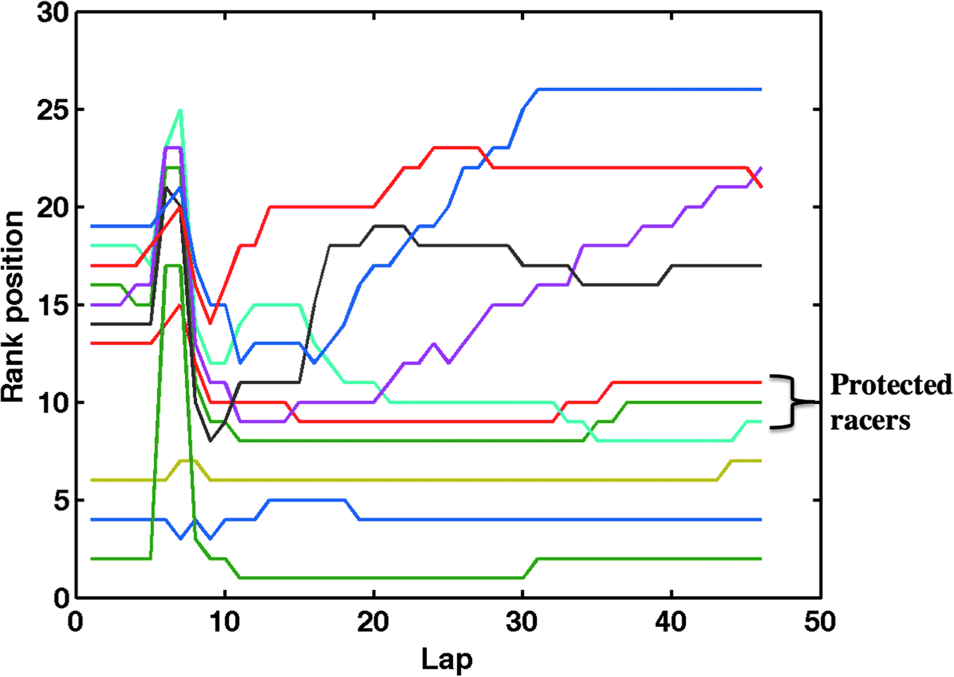
An instance of protection: We plot rank position versus relative lap index for a race. Cars in ranks 2, 4, 6, and 13–19 took two tires and the remaining cars took four tires. For clarity, we show only the rank positions of the cars that took two tires during the sixth/seventh lap. The four-tire cars overtook some of the two-tire cars as seen by the upward moving rank profiles in the upper half of the graph. There were also some two-tire cars that did not change rank position, as seen by horizontal lines in the lower half of the graph. They were thus protected because many of the cars behind them also took two tires.
There are other possible neighborhood effects besides protection. For instance, we hypothesize that the historical performance of a racer's immediate neighbors can help to predict both change in rank and slope of lap times over the course of an epoch. We considered two types of neighbors: neighbors who hold similar rank positions at the beginning of the current outing's pit exit lap**, and neighbors who have held similar rank positions and lap times historically within the race (even if they do not hold similar rank positions in the current outing's pit exit lap). These neighborhood effects help to capture correlations across racers, whereas rank momentum captures temporal correlations.
Aggregation across races can be done, and there are two fundamentally different types of races
Our evidence suggests that it is possible to generalize across races; that is, we can borrow strength from the data of similar races to make improved predictions. This type of across-race regularization helps make the predictive modeling more robust to noise and and helps with the imbalance problem. It is also particularly useful at the start of the race: Using another race's data is better than the alternative, which is no data at all.
“Our evidence suggests that it is possible to generalize across races; that is, we can borrow strength from the data of similar races to make improved predictions.”
Through descriptive statistics, we made the hypothesis that there are fundamentally different types of races, namely, those for which cars typically lose position after a two-tire change (Group A), and those for which cars typically maintain their rank position after a two-tire change (Group B). Thus, in Group B, there is more incentive to take two tires instead of four tires to gain rank positions. In reality, the determination of which group the race belongs to can be done using data from practice and qualifying stages that occur on the same track prior to the race. The fact that our observations are race-specific rather than racer-specific indicates that properties of the track, tires, and weather matter more than racer-specific details in determining how tire-change decisions should be made within a race. In our experiments, we did not explicitly use track-specific information for this clustering and instead used the given lap position and lap time information to come up with the two groups: Group A (with loss in rank pattern) included 6 races and Group B (without loss in rank pattern) included the remaining 11.
Features
Based on the key hypotheses above, we constructed several groups of features for the prediction problem described in The Prediction Problem section.
26
These features heavily rely on the definitions and preprocessing we established in the Preprocessing section. We developed over 100 features, each based on a hypothesis about what might be important for prediction of change in rank over the course of an epoch. The features fall into these categories:
• Basic features: Basic features are constructed from all the historical outings in the data set. These are statistics computed from each outing up to the current outing within the current race and the outings within previous races. Basic features capture (i) the racer's rank position at the decision time and whether his rank position is near the top of the pack or near the bottom. We also include the racer's starting rank position for the race. (ii) The average of the racer's rank positions in previous outings (also various percentiles). This indicates how well the racer is doing generally in the race so far. We also include nonlinear variations of this type of feature, such as the average of the previous rank positions squared. (iii) The age of both the left and the right tires at decision time. (iv) The average of the slopes of the racer's lap times in previous outings based on fits of each “sawtooth” function. This indicates the general speed of wear of tires for that particular racer. We also use nonlinear functions combining the racer's past rank positions and the average slope, which helps to address the nonlinearity due to “fresh air” as discussed above. • Rank momentum features: We compute the minimum, maximum, and average of several rank momentum quantities over previous outings within the race. These features include: change in rank, rate of change in rank, change in rank times average rank, and rate of change in rank times average rank. • Protection features: We compute statistics of the racer's neighborhood. Here, the neighborhood includes cars within a few ranks of the racer's average rank over the course of the immediately previous outing. These statistics include rank momentum features of the neighborhood and can help to determine whether the racer might be near cars that he needs to pass or whether the cars in his neighborhood are likely to be faster than he is, in which case he might lose ranks. We further consider the number of neighbors with zero-, two-, or four-tire changes before their outings began. • Tire decision features: The tire decision that happens before the outing is a critical feature whose impact on the change in rank can help us make decisions during the race. We can make product features from tire-decision features and other features, such as whether the racer has taken two tires and is at the front of the pack in “fresh air.” • Other features: These are features that are potentially important but do not fall into the earlier categories. These features include: – an indicator of first outing in the race. The first outing does not have historical information about past outings of the racer. This makes that outing different from all subsequent outings of the race. – an indicator of pit in caution. This feature allows us to address green lap pit stops differently than pit stops during cautions. – time taken in previous pit stops. This feature addresses the variability in pit times discussed in the Complexities of Racing section. – an indicator variable for whether the previous outing was short. If the previous outing was very short, it may affect the race dynamics in the current outing. Many racers will not change tires if they have done so recently.
Using these features to aggregate information across races assists with the concerns from the Data Issues section specifically, imbalance and the lack of information at the start of a race. It is not true, however, that any past race is able to assist with prediction in any current race; our grouping of tracks alleviates this problem.
Prediction to decision
We built a real-time prediction system by resolving the batch learning problem at each lap. Specifically, to do this for a given racer, at each lap we compute his predicted change in rank position in the next outing given a zero-, two-, or four-tire decision that he may choose to take in a pitstop in the near future. Comparing these three predicted change in ranks against one another helps the crew chief of the team make a well-informed decision.
Experiments
We experimented with several state-of-the art machine learning techniques that permit different combinations of the features we created. In particular, we used ridge regression,††,23 support vector regression (SVR)‡‡,24 with a linear kernel, LASSO (least absolute shrinkage and selection operator),§§,25 as well as random forests for regression
26
and two baselines. Ridge regression and LASSO are very similar techniques in that both use the same least squares loss function, but LASSO uses ℓ1 regularization to determine the coefficients, whereas ridge regression uses ℓ2 regularization. Support vector regression also uses ℓ2 regularization but uses the ε-insensitive loss function. Random forests is an ensemble method that averages predictions from many different decision trees. The two baselines are as follows:
• •
Because we do not have control over data generation as discussed in the Data Issues section, the linear model coefficients (e.g., of support vector regression, ridge regression, and LASSO) cannot be reliably interpreted in the ceteris paribus structural form. This means that if we are to quantify the effect of the tire-decision feature on the subsequent change in rank position, we need the other features to be as orthogonal to the tire-decision feature as possible. Nonetheless, our approach is reasonable as prediction performance is also primarily desired.
Metrics
There are no agreed-upon domain-specific measures of success to employ for our prediction step. We decided to use R2 (r-squared),*** RMSE (root mean squared error) and sign accuracy ††† as the evaluation metrics for the prediction models on out-of-sample data. R 2 describes the proportion of variance of the dependent variable (change in rank position) explained by the regressors (in the Features section) through the prediction model. For a perfect relationship it is 1, and for no relationship it is 0. Sign accuracy captures the proportion of time we predict correctly whether the rank increased, decreased, or stayed the same. Note that if we use a learning algorithm that provides continuous-valued predictions (like Ridge Regression and the LASSO), we will rarely predict exactly zero change in rank; zero change in rank happens about 20% of the time, so the best sign accuracy we can expect is around 80%.
Prediction performance
We performed two sets of experiments using data from all outings that were sufficiently long. The first involves predictive accuracy of the different models. In the second experiment, we observe how the weight of the two-tire indicator feature changes with outing length.
•
•
For both of these experiments, we used five-fold cross validation to set the appropriate regularization coefficient (or parameter values in the case of random forests). We repeated splitting the data into five folds 10 times to make the cross-validation procedure more stable ‡‡‡ and used the same set of folds for all the models used (to control for split variance).
The results of the first experiment characterizing performance of the methods on test data using different metrics are plotted in Figure 9. Figure 10 shows the values of the regularization parameters chosen for each group. The results for the second experiment characterizing the effect of outing length on the model weight of the two-tire change feature are plotted in Figure 11. We summarize some of the findings from these experiments below.
“We can see that the machine learning methods are significantly better than the baseline methods.”
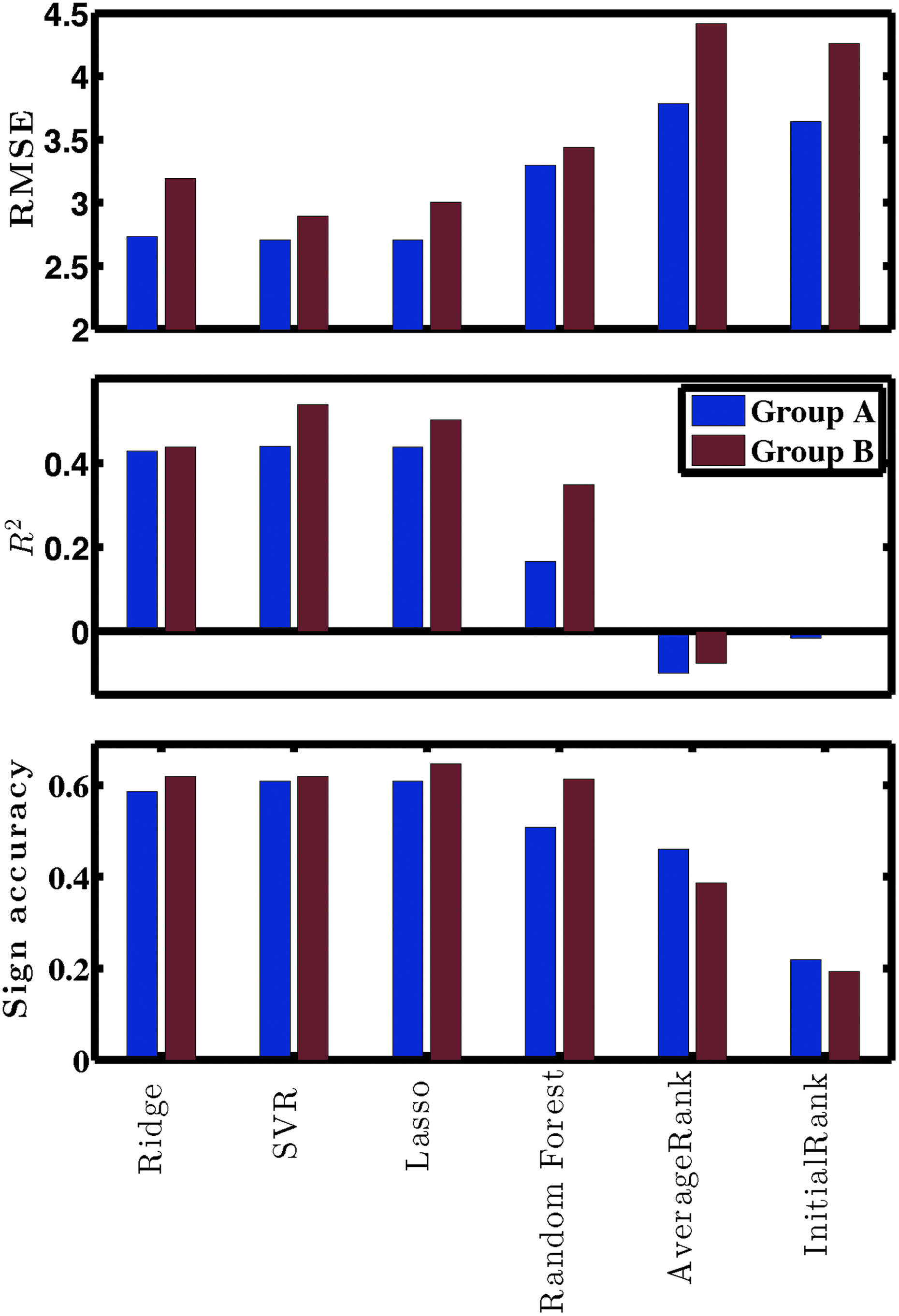
Predictive performance of various models over a held-out test set are shown for races in Group A and Group B. The y-axis plots the RMSE (lower is better) for the top subplot, R2 (higher is better) for the middle subplot, and the sign accuracy (higher is better) for the bottom subplot.
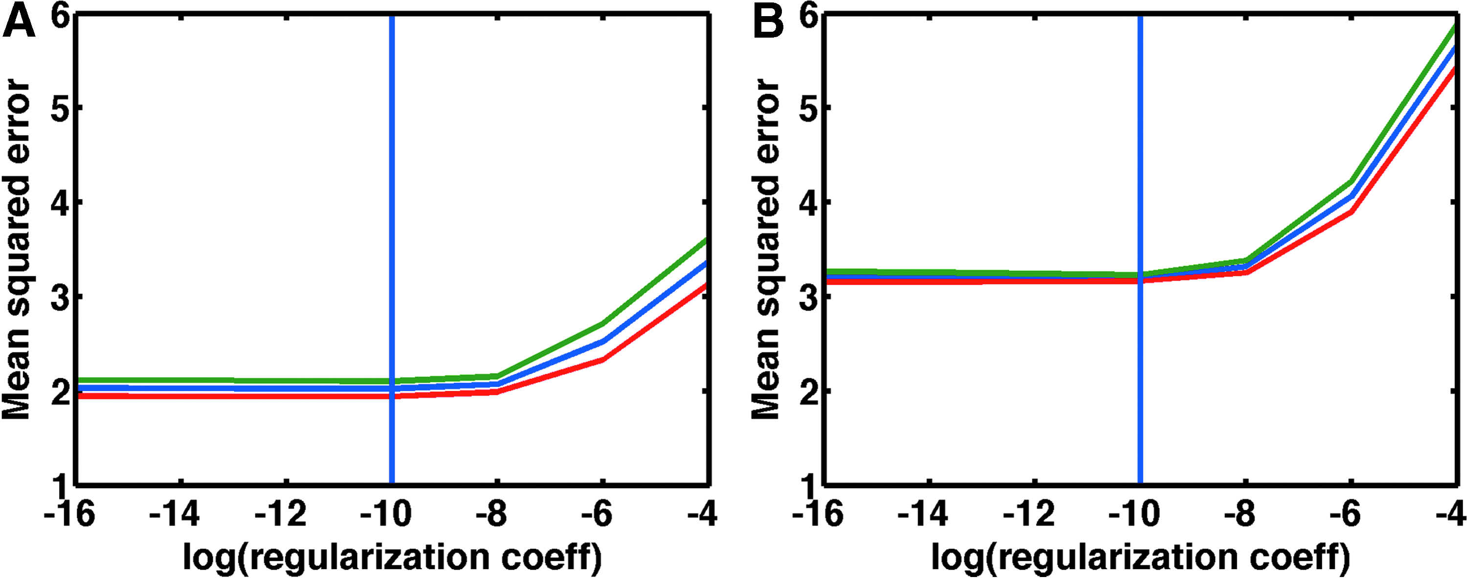
For both groups of races, we plot the mean (over 10 repeated choices of 5 validation sets) of the mean squared error along with error bands corresponding to one standard deviation above and below while building a LASSO model. The vertical line represents the regularization constant for which the mean cross-validation error is the minimum.
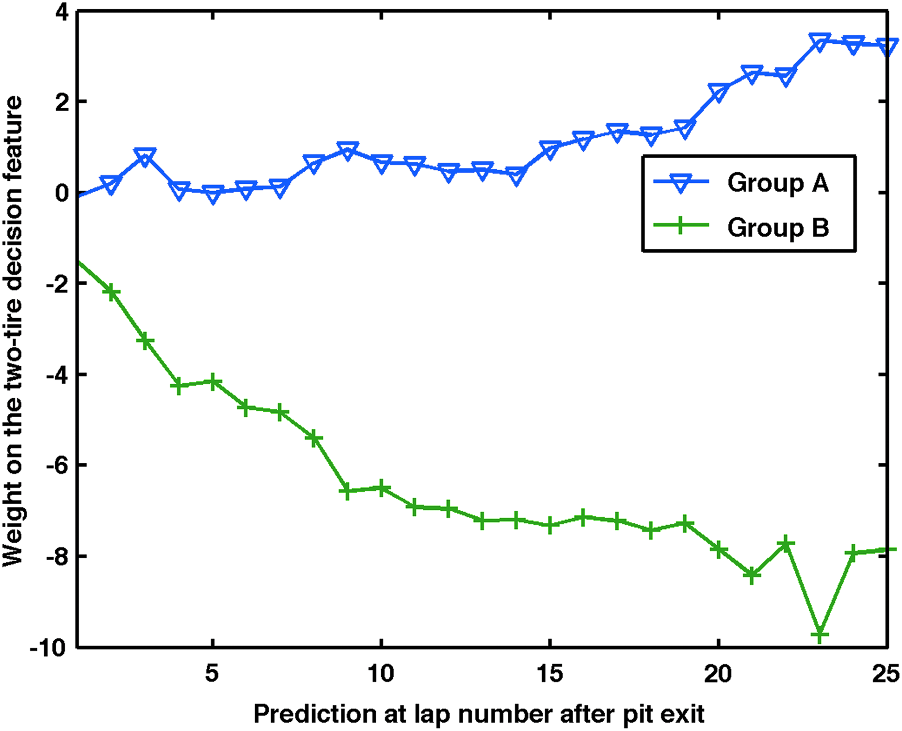
Variation in the weight of the two-tire decision feature in LASSO as a function of the outing length. For Group A, the weight is positive and increasing, indicating that making a two-tire decision increases the change in rank (loss in rank). This effect increases as the outing length increases. An opposite effect is observed in Group B.
Predictive accuracy
• From the prediction performance plots in Figure 9, we can see that the ridge regression, SVR, LASSO, and random forests are significantly better than the baseline methods. The machine-learning methods give very similar held out test set performance. Further reduction in RMSE, increase in R2, and increase in sign accuracy may not be possible because of the highly strategic and dynamic nature of racing.
• Predictions on the test set are somewhat worse than performance on the training set. This is not because of overfitting, it is because the training distribution differs from the test distribution because of the following:
(1) Later outings of a race have different dynamics than the beginning part of the race. For instance, the racers are closer to the finish line in the later outings, so their risk profiles change, leading to more aggressive driving, and typically there are a higher number of cautions.
(2) Two-tire decisions acquire relatively more significance during later outings and are typically observed more during that period of the race. If there are fewer two-tire changes in the earlier part of the race than in the later part, we may not be able to accurately characterize the later part of the race from the earlier part.
Variation of the weight of the two-tire decision feature with outing length
In Figure 11, we see that in Group A (with loss in rank pattern) there is a positive weight on the two-tire change indicator. In Group B (without loss in rank pattern), there is a negative weight on the two-tire change indicator. This effect becomes more extreme as the outing length increases. This really shows the difference between the two groups; the effect of a two-tire change can be quite different.
Some Insights
In this section, we highlight some insights and some cases in which predictive modeling is able to forecast large changes in ranks using historical features.
Predicting outing length is not critical
We find in our experiments that the length of the outing is not an important predictor of change in rank position as long as it is sufficiently long. This is actually quite useful to know as it saves us the trouble of having to forecast outing length, which is very difficult. The reason for outing length not to be necessary could be that, after the initial few laps of a long outing, the racers are typically sufficiently spaced apart on the race track so that the change in rank position remains relatively constant irrespective of the length of the outing.
Note that this observation does not conflict with (and can actually be seen using) Figure 11; as the length of outings increases (toward the right of the figure), the weights stabilize.
It is hard to beat the baseline initial rank with respect to the RMSE
In many of the outings observed, racers typically change their position by zero, one, or two ranks. Thus the baseline trivial model that predicts zero change in rank all the time does fairly well with respect to the RMSE. It does not, however, perform well with respect to the R2 or sign accuracy metrics. In fact, since it always predicts zero, and cars stay in the same rank position about 20% of the time, the sign accuracy is 20%.
Validation through expert commentary
Expert commentaries
§§§
that are typically stated either before or after the race can also be used to qualitatively validate the inferences of our modeling approach. For example, some commentaries about the characteristics of tracks that influence racing strategies and outcomes for 2012 were:
• “As your fuel load burns off, you gain a little bit of speed on track…the tires aren't falling off much…” • “I don't think tire wear is going to be very high…” • “Tires don't really seem to be making a huge difference in lap times…” • “…crew chiefs must decide whether to pit or not and whether to take two tires or four.” • “…you are going to see two tires, you are going to see four tires…”
When we looked at the tracks that the experts were commenting on, we found that the first three comments corresponded to tracks in Group B. Recall that Group B includes tracks for which the number of tires changed tends not to matter, and where we recommended taking two tires rather than four because there is no loss in rank pattern. Our grouping agreed with the expert commentary in all three cases. The last two comments corresponded to tracks in Group A, where we correctly identified that there was a perceivable effect of a two-tire strategy on rank position outcomes.
“Expert commentaries that are typically stated either before or after the race can also be used to qualitatively validate the inferences of our modeling approach.”
There are other types of commentaries that are useful in decision making but are not directly related to our grouping. For instance, some tracks have far-spaced and few caution lap periods. This is because the track is wide, which reduces the possibility of cautions and in turn affects the tire strategy of racers. Thus, these commentaries also help to justify our clustering of races before fitting the prediction models.
Insights for some extreme outings observed in the dataset
It is of particular interest to the teams to understand outings in which a high change in rank occurs. We now present some representative cases in which change in rank was significantly high and moderately predictable. See Table 2 for a numerical summary of these cases. We qualitatively describe why our prediction model (in particular, LASSO) was able to predict these “high” change-in-rank cases. LASSO outputs a linear model; that is, it provides a weight for each feature, and the weighted sum of features is the predicted change in rank. These weights can be positive or negative.
Negative change in rank values mean that the racer gained positions by the end of the outing compared to the pit entry before the outing. All the outings here are toward the end of the race.
Fifth outing for car #5 in a race in the southern United States
Our model pinpointed two main reasons why this particular racer should gain ranks in the next epoch. This racer was toward the back of the pack, and his tires did not wear out as quickly as the other racers in the previous epoch (as indicated by the slope of his lap times). To show how our model does this, we note first that the feature rank(pit entry lap) encodes that his rank is toward the back. Second, we note that the feature slope(laptimes of previous outing)×rank(pit exit lap) incorporates the fact that his tires did not wear out as quickly as usual for someone in his rank through a low slope in lap times. Further, this race is in Group B, which means that two-tire changes do not cause as many losses in rank position. As it turns out, in this epoch, the racer took two tires; we predicted that with this choice he would gain a large number of rank positions (10.36), and he gained an even larger number of rank positions (17).
Fifth outing for car #31 in a race in the southern United States
This racer was near the front of the pack, and in the previous outing, his slope was relatively high for his rank, indicating that his tires were wearing out more quickly than other racers. Because of this, again our model used the features rank(pit entry lap) and slope(laptimes of previous outing)×rank(pit exit lap) to predict that he would lose a lot of ranks over the next outing. He took zero tires, and we predicted that he would lose 6.11 ranks; he lost 13 ranks.
Fifth outing for car #2 in a race in the northern United States
Similar to the previous case, this racer was near the front of the pack through most of the race. But in contrast, his slope was relatively low for his rank in the previous outing, indicating that he had a fast car or his tires were wearing out slower than other racers. In particular, our model used the most dominating feature slope(laptimes of previous outing)×rank(pit exit lap) to predict that he would gain ranks over the next outing. He took two tires, and we predicted a gain of 2.88 ranks whereas in reality, he gained 5 ranks.
Eighth outing for car #29 in a race in the southern United States
This racer alternated between being near the front of pack and being near the back of the pack in his previous outings. His rank was low at pit entry for the outing of interest here. In addition, in the immediate previous outing, his lap times had a high slope (indicating a slower car or relatively more tire wear). Our model used the features rank(pit entry lap) and slope(laptimes of previous outing)×average-rank(previous outing) to predict that he would lose ranks over the next outing. We predicted a loss of 3.77 ranks and the ground truth was that he lost 10 ranks (and took two tires before the outing).
In all the above cases, many other features were also influencing the change (loss) in rank variable, including features related to the past two-tire and four-tire changes, slope(laptimes of previous outing)×final-rank(previous outing), and functions like square root and square of final-rank(previous outing) among others. Their influence was relatively smaller for these outings.
Conclusions
We describe challenges in formulating a prediction problem that leads into the design of decision-making tools for strategic use within a professional sporting event. Careful use of domain knowledge and transformation of time series data into a supervised learning framework were the key aspects in our ability to do this. We demonstrated the validity of our prediction models using data from a professional racing season in 2012.
Footnotes
Author Disclosure Statement
No competing financial interests exist.
Acknowledgments
We would like to thank Fabrice Vegetti and several others from whom we enjoyed learning about racing. We would also like to thank Claudia Perlich for her comments, which helped improve this article.
References
 . Shave Magazine races? Sprint Cup series: The impact of multi-car teams. Social Science Research Network races: The role of driver experience