Bigger is Better,but at What Cost? Estimating the Economic Value of Incremental Data Assets

Abstract

Abstract

Many firms depend on third-party vendors to supply data for commercial predictive modeling applications. An issue that has received very little attention in the prior research literature is the estimation of a fair price for purchased data. In this work we present a methodology for estimating the economic value of adding incremental data to predictive modeling applications and present two cases studies. The methodology starts with estimating the effect that incremental data has on model performance in terms of common classification evaluation metrics. This effect is then translated into economic units, which gives an expected economic value that the firm might realize with the acquisition of a particular data asset. With this estimate a firm can then set a data acquisition price that targets a particular return on investment. This article presents the methodology in full detail and illustrates it in the context of two marketing case studies.

Introduction

In commercial predictive modeling applications, data almost always comes at a price. This is certainly true in many marketing scenarios where companies can purchase consumer data from third-party vendors. A common question for managers and data scientists building predictive systems is, “How much is a particular set of data worth?”

Most data vendors sell data at a fixed price and leave it to the buyers to determine if the data holds enough value to justify that price. Despite the prevalence of this problem in data-driven businesses, there is very little research to guide buyers in how to effectively price available data sources. A study by the Organization for Economic Cooperation and Development ¹ surveys several methods for determining the economic worth of a data point, but these are generally framed from the seller's perspective (such as using market clearing price or total revenues divided by total data points). From the buyer's perspective, the true value of data should be a function of its ability to predict future outcomes and not just explain the past. ² In this regard, it is important to formulate the problem of data valuation using the tools of predictive modeling.

In this article, we show how common predictive modeling metrics can be expressed in terms of the expected economic gain or loss (value) of taking some action based on the prediction a model makes on an instance. With these metrics translated into economic units, we can show how changes in these metrics, induced by adding data, relate to the value created by such data. Once we can quantify how new data might change the expected value of applying a predictive model, we can then make better managerial decisions on what return on investment (ROI) the new data might generate.

“Our data valuation methodology works by turning prediction into action and then evaluating the economic impact of those actions.”

Our data valuation methodology works by turning prediction into action and then evaluating the economic impact of those actions. New data changes how we might act on an instance, and there are economic implications to that change of action. We propose that the value of a data point should be related to this change, and our method is designed to express this in a mathematical way. We introduce our methodology from the point of view of general predictive modeling and then illustrate it using two case studies from real-world data sets. The first covers a recurring data acquisition decision by Dstillery, an Internet display advertising firm (and the authors' present affiliation). The second example uses data from the 1998 ACM SigKDD conference data mining competition and explores the data valuation process for a charity's direct mail campaign. In both examples, we price externally available data under two scenarios: (1) where proprietary data is available; (2) where it is not. We find that the predictive power of external data available for purchase changes dramatically in the presence of useful proprietary data, and the price a firm should be willing to pay for such data changes accordingly.

Related Work

The value of data in a nonmonetary sense has been considered in many disciplines, including statistics, machine learning, and predictive modeling for different scenarios:

• Feature selection assesses the value of existing features and considers the impact of removing them for the sake of either model performance or parsimony.^3,4

• Learning curve analysis focuses on how having more examples (features plus labels from the same distribution) affects the model performance.^5,6

• Active learning aims to selectively acquire training labels for supervised learning in a way that maximizes performance gains while minimizing label acquisition costs. ⁷

• Active information acquisition considers the selective purchase of features during both training and model use. ⁸

• Cost-sensitive classification aims to determine classifier thresholds that minimize the expected economic costs of applying the classifier.^9–11

In nearly all cases of existing research, the value of data is defined with respect to its impact on some model performance metric rather than the monetary implications of the decision being made using the model. ⁸ The exception is with cost-sensitive classification, which considers the costs of different types of classification error and proposes schemes to minimize these costs. Our process for estimating the value of data combines the economic elements of cost-sensitive classification with methods common in feature selection and active information acquisition.

In this work, we aim to estimate the expected economic impact of straightforward cases of feature acquisition. We link improved model performance to monetary gain by connecting common performance metrics to monetary units. This enables us to explore the full impact of data acquisition on revenue and profit, which informs strategic decisions during negotiations with data providers.

Estimating the Value of Data

The process of quantifying the monetary value of data involves (1) framing the problem, that is, defining the mechanism for translating model predictions into decisions/actions and associating different costs/payoffs depending on the various outcomes; (2) identifying an appropriate nonmonetary performance metric for a given application; and (3) defining a mechanism for quantifying the impact that an incremental data unit has on model performance for the (holdout) use cases. These steps are detailed in the next few sections and then illustrated with two cases on real data.

Framing the problem

We narrow the scope of our analysis to applications involving tasks with binary outcomes (e.g., the customer responds to an offer or not) with models that predict a continuous score (i.e., the probability of one of the two outcomes). We first formally define a classifier F as a continuous scoring function \documentclass{aastex}\usepackage{amsbsy}\usepackage{amsfonts}\usepackage{amssymb}\usepackage{bm}\usepackage{mathrsfs}\usepackage{pifont}\usepackage{stmaryrd}\usepackage{textcomp}\usepackage{portland, xspace}\usepackage{amsmath, amsxtra}\pagestyle{empty}\DeclareMathSizes{10}{9}{7}{6}\begin{document} $$\hat{s} = g ( X )$$ \end{document} (for now we are agnostic to the choice of scoring function), a threshold k, and a binary indicator function \documentclass{aastex}\usepackage{amsbsy}\usepackage{amsfonts}\usepackage{amssymb}\usepackage{bm}\usepackage{mathrsfs}\usepackage{pifont}\usepackage{stmaryrd}\usepackage{textcomp}\usepackage{portland, xspace}\usepackage{amsmath, amsxtra}\pagestyle{empty}\DeclareMathSizes{10}{9}{7}{6}\begin{document} $$\hat{Y} = I ( \hat{s} > k )$$ \end{document} that assigns a class (which is linked to an action) to a given instance based on its feature vector X.

There are many suitable evaluation metrics for the type of classification system defined above, and the appropriate evaluation metric is problem dependent. The exact use of the model is the defining factor in making this choice, and it also influences our economic analysis of the problem. The following list provides some examples of common economic applications of classification systems:

1. With a fixed budget, take action on exactly T instances. This is a scenario in which a classification system is used to define a ranked list, and the classification threshold k is chosen to classify exactly T instances as positive. The objective in such a scenario is to maximize the number of true positives (TPs; instances that indeed were of the positive class) in the top T instances. The appropriate metrics are precision (percentage of TP examples in the list of P instances) or lift (relative number of TPs compared to the number of expected TPs expected at random, which is equivalent to a normalized precision measure). The economic interpretation of this strategy is to maximize revenue given a fixed cost of action.

2. Given an open budget, take action while the expected benefit of action is above some minimum threshold (e.g., cost or profit maximization). This is again a scenario where a ranked list is appropriate (but not necessary). The classification threshold for the action can be set by choosing k such that E[value]>δ, and appropriate metrics would be area under the ROC curve ¹¹ (AUC) or log-likelihood score.

3. Given a ranked list, choose a threshold k such that an exact number of TPs has been acquired. In this scenario, the appropriate metric is recall (formally, the percentage of positives above k), and the economic interpretation is to minimize the cost of acquiring a set number of TPs.

4. Apply 1 and 3 above, but with uncertainty about the budget. The ranking model is built in advance, but the budget, which is a determining factor of the classification threshold k, is not set, and it is assumed to take on arbitrary values with equal likelihood. In these cases, again AUC is an appropriate metric.

Let m( \documentclass{aastex}\usepackage{amsbsy}\usepackage{amsfonts}\usepackage{amssymb}\usepackage{bm}\usepackage{mathrsfs}\usepackage{pifont}\usepackage{stmaryrd}\usepackage{textcomp}\usepackage{portland, xspace}\usepackage{amsmath, amsxtra}\pagestyle{empty}\DeclareMathSizes{10}{9}{7}{6}\begin{document} $$D , \hat{s} , \hat{Y}$$ \end{document} ) be an evaluation function that computes some appropriate evaluation metric (e.g., precision, recall, or AUC) on a holdout data set D using the output of the classifier F. Our first question of interest is, “How does incremental data affect m( \documentclass{aastex}\usepackage{amsbsy}\usepackage{amsfonts}\usepackage{amssymb}\usepackage{bm}\usepackage{mathrsfs}\usepackage{pifont}\usepackage{stmaryrd}\usepackage{textcomp}\usepackage{portland, xspace}\usepackage{amsmath, amsxtra}\pagestyle{empty}\DeclareMathSizes{10}{9}{7}{6}\begin{document} $$D , \hat{s} , \hat{Y}$$ \end{document} )?”

We first answer this by defining exactly what we mean by incremental data. Let D be an N×M+1 data matrix that consists of N examples, M features, and an outcome Y. We can partition our matrix as follows: \documentclass{aastex}\usepackage{amsbsy}\usepackage{amsfonts}\usepackage{amssymb}\usepackage{bm}\usepackage{mathrsfs}\usepackage{pifont}\usepackage{stmaryrd}\usepackage{textcomp}\usepackage{portland, xspace}\usepackage{amsmath, amsxtra}\pagestyle{empty}\DeclareMathSizes{10}{9}{7}{6}\begin{document} \begin{align*} D = [ X^{ \rm BL} \ X^{ \rm Inc} \ Y ] \end{align*} \end{document}

The superscripts BL and Inc indicate disjoint sets of features/columns, and each can be of any arbitrary dimension. As a result, M=M^BL+M^Inc. Let D^BL be a baseline data matrix that consists of only baseline features and the target [X^BL Y]. Let D^Inc be a new data set that includes D^BL but is augmented by the columns X^Inc.

“Our objective is to measure the impact of adding this new X^Inc data to our evaluation metric.”

Our objective is to measure the impact of adding this new X^Inc data to our evaluation metric. We define a quantity that represents the counterfactual (the effect on our metric of the incremental data). \documentclass{aastex}\usepackage{amsbsy}\usepackage{amsfonts}\usepackage{amssymb}\usepackage{bm}\usepackage{mathrsfs}\usepackage{pifont}\usepackage{stmaryrd}\usepackage{textcomp}\usepackage{portland, xspace}\usepackage{amsmath, amsxtra}\pagestyle{empty}\DeclareMathSizes{10}{9}{7}{6}\begin{document} \begin{align*} \Delta m = m ( D^{{ \rm Inc}} , \hat{s}^{{ \rm Inc}} , \hat{Y}^{{ \rm Inc}} ) - m ( D^{{ \rm BL}} , \hat{s}^{{ \rm BL}} , \hat{Y}^{{ \rm BL}} ) \end{align*} \end{document}

In defining Δm, we assume that D, \documentclass{aastex}\usepackage{amsbsy}\usepackage{amsfonts}\usepackage{amssymb}\usepackage{bm}\usepackage{mathrsfs}\usepackage{pifont}\usepackage{stmaryrd}\usepackage{textcomp}\usepackage{portland, xspace}\usepackage{amsmath, amsxtra}\pagestyle{empty}\DeclareMathSizes{10}{9}{7}{6}\begin{document} $$\hat{s}$$ \end{document} , and \documentclass{aastex}\usepackage{amsbsy}\usepackage{amsfonts}\usepackage{amssymb}\usepackage{bm}\usepackage{mathrsfs}\usepackage{pifont}\usepackage{stmaryrd}\usepackage{textcomp}\usepackage{portland, xspace}\usepackage{amsmath, amsxtra}\pagestyle{empty}\DeclareMathSizes{10}{9}{7}{6}\begin{document} $$\hat{Y}$$ \end{document} are out-of-sample (not used for model training), and that the same features used in training are available for evaluation as well. We also point out that with the augmented data set, we have a scoring model and as a result a new classifier, which we have identified with the appropriate superscripts.

Counterfactual analysis has long been used as the default tool for measuring causal relationships in both experimental design and observational studies.^12–14 The use of this method has long been a standard for feature selection, ³ feature importance, ¹⁶ and active learning ⁷ applications, and is even built into commonly used training algorithms. ¹⁷ We rely on this tool based on its extensive support in the literature and its extensibility to economic analysis of machine learning metrics. Intuitively speaking, we are simulating what would have happened to the model performance if we had had the incremental data bought already. This analysis assumes that the data is available at no or limited cost for a trial before making the final purchase decision.

Classification metrics in monetary terms

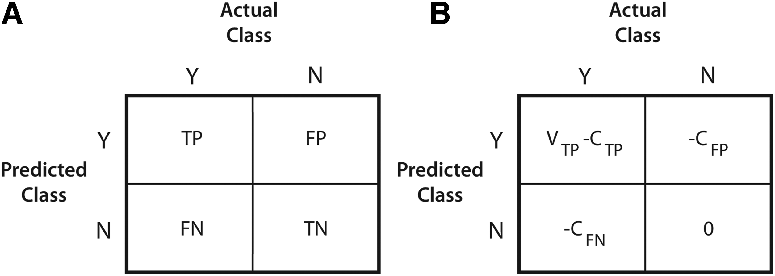
For any of the above economic applications, we need a way to express the expected economic value of taking an action for an instance as a function of Δm. We start by considering the confusion matrix derived from comparing the predicted class with the actual class/outcome of the instance in the set of actions based on a cutoff k.

We generally assume that a true positive (TP) (the number of positives above k), false positive (FP, the number of negatives above k), false negative (FN, number of positives below k), and true negative (TN, number of negatives below k) have a constant cost or economic gain associated with them, which we represent in the cost–confusion matrix of Figure 1. We admit that accurately specifying the figures in the cost–confusion matrix is often a nontrivial task, but for now we assume that these are known.

FIG. 1.

The confusion (A) and cost–confusion (B) matrices are helpful tools for setting up various classification metrics, as well as understanding the economic implications of classification decisions.

We next define a value E_F[V_i], which is the expected value of applying our classifier to a test instance i. E_F[V_i] is a real valued quantity that has units in some form of tangible currency. We focus our analysis at the instance level to decouple the size of the classification application from the classification of particular instances. Our goal is to express E_F[V_i] in terms of our evaluation function m(D, \documentclass{aastex}\usepackage{amsbsy}\usepackage{amsfonts}\usepackage{amssymb}\usepackage{bm}\usepackage{mathrsfs}\usepackage{pifont}\usepackage{stmaryrd}\usepackage{textcomp}\usepackage{portland, xspace}\usepackage{amsmath, amsxtra}\pagestyle{empty}\DeclareMathSizes{10}{9}{7}{6}\begin{document} $$\hat{s}$$ \end{document} , \documentclass{aastex}\usepackage{amsbsy}\usepackage{amsfonts}\usepackage{amssymb}\usepackage{bm}\usepackage{mathrsfs}\usepackage{pifont}\usepackage{stmaryrd}\usepackage{textcomp}\usepackage{portland, xspace}\usepackage{amsmath, amsxtra}\pagestyle{empty}\DeclareMathSizes{10}{9}{7}{6}\begin{document} $$\hat{Y}$$ \end{document} ) so that we can ultimately express the change in expected value (ΔE_F[V_i]) as a function of Δm. The price one should pay for incremental data should ultimately be a function of how that data changes the expected value of the application of that data.

We now define changes in E_F[V_i] explicitly in terms of changes in precision, lift, recall, AUC, and partial AUC. In the next section, we present just the main results for concision. The full derivations can be found in the Appendix.

Precision/lift

Precision at a threshold k represents the percentage of instances classified as positive that are indeed positive and is defined as: PRE _k =TP×(TP+FP)⁻¹. Lift at the same threshold k is just the precision at k divided by the base percentage of positives in the entire dataset (not just the set above k). Since the precision and lift vary by a constant scalar, we consider only precision for the rest of this analysis.

Given two classifiers F_k^Inc and F_k^BL, we can now express the change in expected value from using the former over the latter as a function of the change in precision. Specifically, \documentclass{aastex}\usepackage{amsbsy}\usepackage{amsfonts}\usepackage{amssymb}\usepackage{bm}\usepackage{mathrsfs}\usepackage{pifont}\usepackage{stmaryrd}\usepackage{textcomp}\usepackage{portland, xspace}\usepackage{amsmath, amsxtra}\pagestyle{empty}\DeclareMathSizes{10}{9}{7}{6}\begin{document} \begin{align*} \Delta E_k [ V_i ] = E_k [ V_i \mid {\rm PRE}_k^{{ \rm Inc}} ] - E_k [ V_i \mid { \rm PRE}_k^{{ \rm BL}} ] \\= \Delta { \rm PRE}_k \times ( V_{{ \rm TP}} - C_{{ \rm TP}} + C_{{ \rm FP}} ) \end{align*} \end{document}

where ΔPRE _k =PRE _k ^Inc−PRE _k ^BL.

Recall

Recall (also called the TP rate) at a threshold k represents the percentage of TPs within the top k and is defined as: REC _k =TPR _k =TP/(TP+FN). To express ΔE_k[V_i] in terms of ΔTPR _k , we need to also introduce the FP rate at threshold k (FPR _k ), defined as FPR _k =FP/(FP+TN).

Thus, for a fixed FPR _k : \documentclass{aastex}\usepackage{amsbsy}\usepackage{amsfonts}\usepackage{amssymb}\usepackage{bm}\usepackage{mathrsfs}\usepackage{pifont}\usepackage{stmaryrd}\usepackage{textcomp}\usepackage{portland, xspace}\usepackage{amsmath, amsxtra}\pagestyle{empty}\DeclareMathSizes{10}{9}{7}{6}\begin{document} \begin{align*}\Delta E_k [ V_i ] = p ( Y ) \times \Delta { \rm TPR}_k \times ( V_{{ \rm TP}} - C_{{ \rm TP}} + C_{{ \rm FN}} ) \end{align*} \end{document}

where ΔTPR _k =TPR _k ^Inc−TPR _k ^BL.

Without this constraint, we would need knowledge of both metrics to compute the change in expected value: \documentclass{aastex}\usepackage{amsbsy}\usepackage{amsfonts}\usepackage{amssymb}\usepackage{bm}\usepackage{mathrsfs}\usepackage{pifont}\usepackage{stmaryrd}\usepackage{textcomp}\usepackage{portland, xspace}\usepackage{amsmath, amsxtra}\pagestyle{empty}\DeclareMathSizes{10}{9}{7}{6}\begin{document} \begin{align*} \Delta E_k [V_i] = p (Y) \times \Delta {\rm TPR}_k \times (V_{{ \rm TP}} - C_{{ \rm TP}} + C_{{\rm FN}}) - p (N) \\ \quad \times \Delta { \rm FPR}_k \times C_{\rm FP} \end{align*} \end{document}

where ΔFPR _k =FPR _k ^Inc−FPR _k ^BL.

Some applications might call for minimizing the cost of acquiring a set number of TPs. In such cases, we seek to lower the FPR given a fixed TPR. This amounts to setting ΔTPR _k =0 and just using the right-most term in the above equation.

Area under the ROC curve

The receiver operator curve is a plot of the points (TPR _k , FPR _k ) of a given classifier F for every possible threshold value k. The AUC is a metric that defines the general ranking ability of a classifier across all instances. The AUC is also equivalent to the Mann–Whitney U statistic and represents the probability that a positively labeled instance has a higher score than a negatively labeled instance.

The AUC is an appropriate metric under scenarios where the exact classification threshold k might not be known in advance. This scenario is likely under budget uncertainty, when at the time of evaluating a predictive model, one does not know exactly the size of the population to which it will be applied. Another use case of the AUC is when data sets are sold in bulk such that all instances must be purchased. An ideal scenario is one where we can cherry pick the best instances (i.e., the instances that our classifier would predict to be positive), but we do not often have this option. In such circumstances, we need to quantify the average expected value of all instances.

We adjust the above notation to express this uncertainty over the threshold k. E_k[V_i] gives us the expected value of applying a classifier with a known threshold k on an instance. We now define E[E_k[V_i]] as the expected value of E_k[V_i] over all possible values of k.

With this quantity defined, we can relate the change in expected value to the change in AUC: \documentclass{aastex}\usepackage{amsbsy}\usepackage{amsfonts}\usepackage{amssymb}\usepackage{bm}\usepackage{mathrsfs}\usepackage{pifont}\usepackage{stmaryrd}\usepackage{textcomp}\usepackage{portland, xspace}\usepackage{amsmath, amsxtra}\pagestyle{empty}\DeclareMathSizes{10}{9}{7}{6}\begin{document} \begin{align*} \Delta E [E_k [V_i]] = (V_{{ \rm TP}} - C_{{ \rm TP}} + C_{{ \rm FN}}) \times p (Y) \times \Delta {\rm AUC} \end{align*} \end{document}

where ΔAUC=AUC^Inc−AUC^BL.

In situations where k is unknown but can be restricted to some range based on domain knowledge of the problem, the partial-AUC ¹⁸ can be used in the above equation.

Case Studies

“We have presented our methodology being agnostic to model estimation, but it should be noted that the algorithm/model used could have a dramatic effect on the final value estimates.”

In this section we present two case studies on real data that demonstrate our data pricing methodology. To recap our method, the estimation of the economic value of data begins first by defining exactly what is incremental data, determining an appropriate metric given the application, and defining values for the different cells in the cost–confusion matrix. The second step is to estimate two models, one without the incremental data and another with it. We have presented our methodology being agnostic to model estimation, but it should be noted that the algorithm/model used could have a dramatic effect on the final value estimates. Last, given both models, compute the difference in the desired metric and apply one of the formulas presented in the section Estimating the Value of Data.

We illustrate this methodology on the following classification scenarios:

1. Dstillery display advertising: We estimate the value of augmenting display advertising campaign decisions with third-party audience segments.

2. Direct mail campaign: We estimate the value of adding data for predicting response rates in a direct mail campaign soliciting donations to a veteran's charity.

Case study 1: display advertising

Dstillery is an advertising technology company that uses predictive modeling to define audience segments for display advertising. ¹⁹ The company uses both first-party and third-party user behavior data to match the right ads to the right users. As is common in the ad tech industry, Dstillery has its own native data but also has access to data segments sold by third parties. The optimization scenario we present here is one in which we want to target a specified number of users and minimize the total cost per acquisition, which is the cost of media plus data divided by total conversions. The metric we focus on is precision at 1% of the scored sample.

For this example, we cover a common scenario the firm faces when managing campaigns—given our own proprietary data, should we purchase any additional third-party data to improve campaign performance? We illustrate this scenario by estimating the performance improvement of adding 1 of 4 third-party audience segments ¹⁵ to each of 10 campaigns. We examine this under two scenarios: (1) where no prior data is available; (2) where the default Dstillery data is available. The second scenario best represents how our analysts would approach the problem in normal operations. We run the first to highlight a very important point—some data alone has demonstrable value, but conditional on other data being present, that value can be diminished.

Figure 2 shows the estimated value of 4 third-party segments for 10 campaigns under the first scenario (i.e., no other data available). In this analysis, we calculate ΔPRE. We do not need a prediction model here because the baseline is the base conversion rate (equivalent to a model without any features), and the incremental data is defined as a user being in a single particular segment.

FIG. 2.

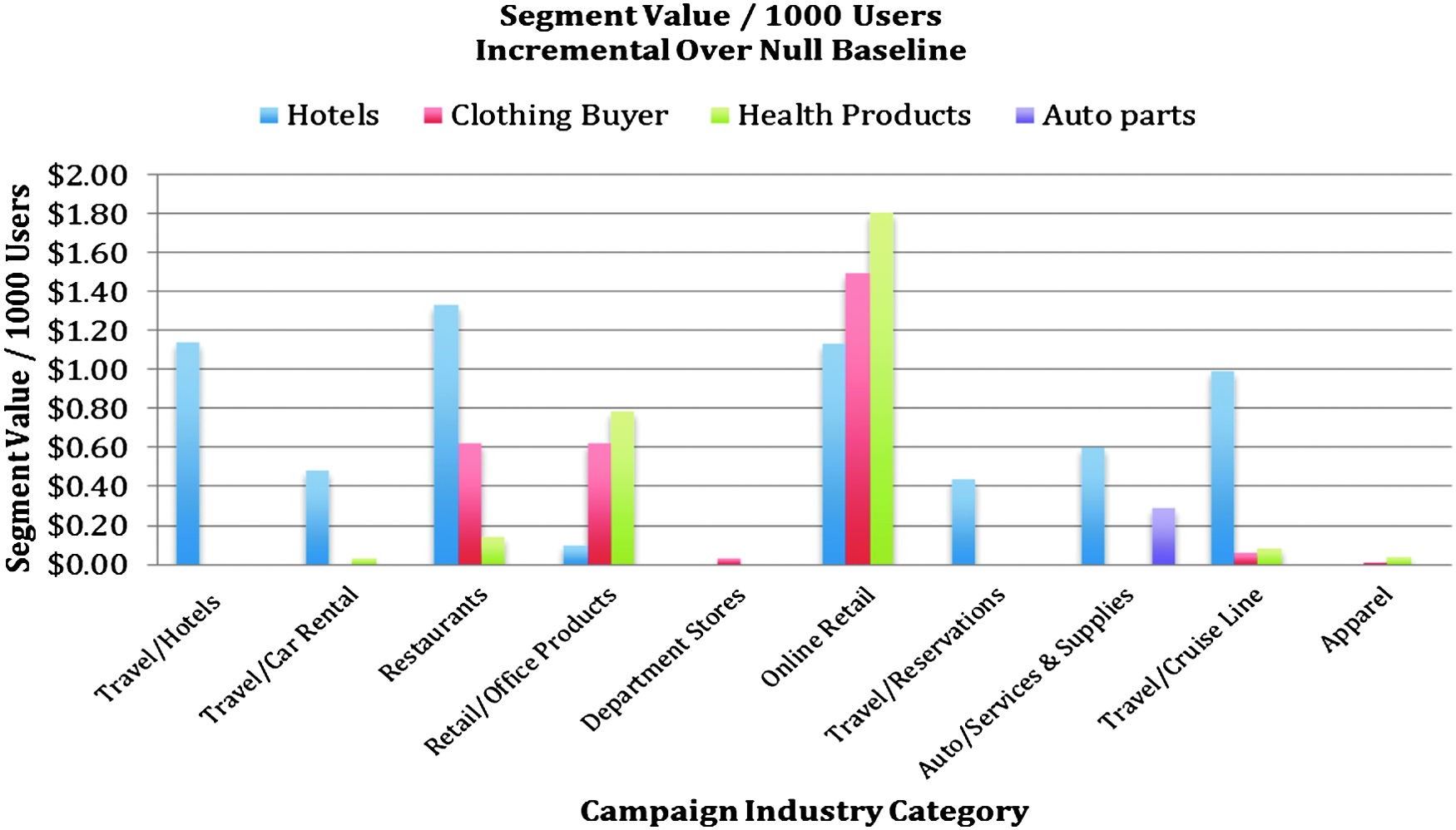
The incremental value of targeting a user in a particular segment across 10 different campaigns. The incremental value is relative to randomly targeting users and is represented as the value per 1000 users targeted. The value of a conversion is different for each campaign, but ranges from $200 for the cruise line to $1.50 for restaurants. For the purpose of this analysis, we assumed that the media cost is the same for users in the segment as it is for randomly targeted users.

We can see in this figure that each segment has a different value for each campaign, and a given segment can be worth a lot for one campaign and nothing for another. The variances are a function of both differing values per conversion and the fact that segments are naturally more suited for certain campaigns (e.g., we find the auto parts intender segment has value only for the campaign selling auto supplies).

The values shown in Figure 2 can be used by a campaign account manager as a decision tool for whether to purchase a particular segment for a given campaign. Given the assumed value of conversion and cost of media, if the cost of data is less than the value estimated by our methodology, then purchasing the data represents a positive ROI decision.

We next perform the same analysis using as a baseline the data that is native to the Dstillery system. This data consists of consumer web usage that contains the URLs visited by a particular consumer in a particular period of time. This data is partially purchased in batch from third parties and partially obtained for free as a byproduct of bidding activity. In effect, this data can be considered a sunk cost. In this experiment, we train L2 regularized logistic regression models ²⁰ with two groups of features: (1) binary indicators of user membership in any Dstillery owned and defined segment; (2) binary indicator of the user membership in the particular third-party segment we are evaluating. The estimates were derived using precision values calculated from an out-of-sample holdout set.

Figure 3 replicates Figure 2 with the new baseline model. We can see in Figure 3 that for the particular campaigns and segments chosen for this analysis, the incremental value of the data changes dramatically once we include Dstillery data. In most cases, the incremental value goes to zero. In general, this type of phenomenon is driven by redundancies in the incremental data. We see that the third-party segments have value when used alone, but conditional on some other data being present, the value is dramatically reduced.

FIG. 3.

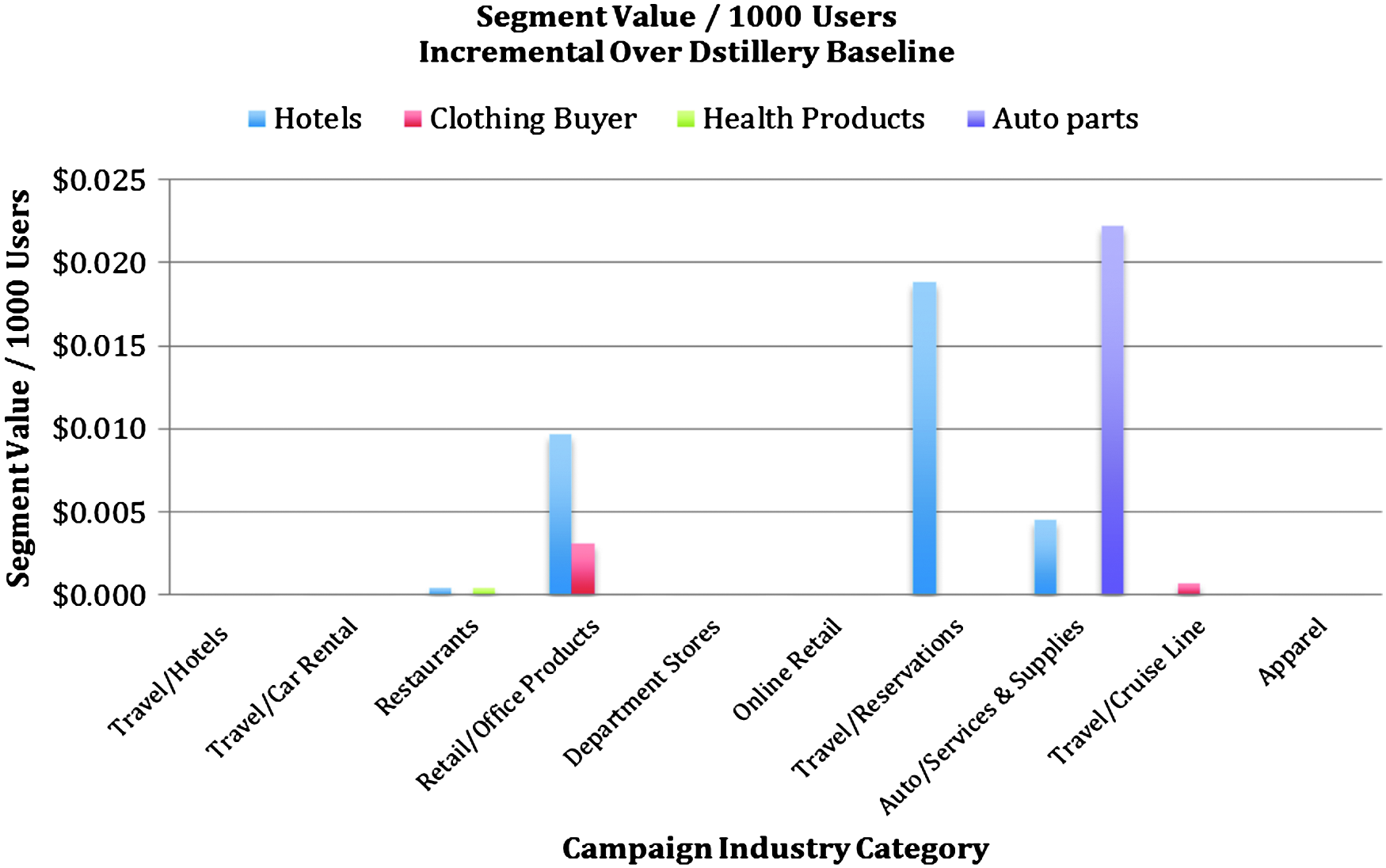
The incremental value of targeting a user in a particular segment across 10 different campaigns. The incremental value is over the performance achieved by using Dstillery's default data and is represented as the value per 1000 users targeted. In each case, we examine the precision when targeting the top 1% of the scored user base for models with and without the indicated segment.

Case study 2: direct mail donation solicitations

In this example, we examine another targeted marketing scenario, but the data acquisition process is different from the first setting. In the display advertising scenario presented above, a firm pays for the data only if the user is in the segment. In this sense the data can be cherry picked such that only users with some positive expected value are selected. In other cases, data is sold as an all-or-nothing scenario. In such a scenario, the firm buying the data has to buy a set of features for all users and only after the purchase can the buying firm decide who to target.

The dataset used is from the second KDD CUP in 1998. It was provided by the Paralyzed Veterans of America (PVA), a not-for-profit organization that provides programs and services for U.S. veterans with spinal cord injuries or disease. With an in-house database of over 13 million donors, PVA was also one of the largest direct mail fundraisers in the country. The dataset provided for the contest consists of 191k “lapsed” donors who are individuals that made their last donation to PVA 13–24 months prior to the date of the data.

We chose this dataset as a relevant case study because it contains very rich groups of features from different origins, is a well-defined predictive modeling problem, and contains known values for the quantities in the cost–confusion matrix.

The dataset has five groups of features, two of which are internal to PVA (base and historical) and three are external (census and two third-party sources):

• Base: information on the household including demographic data such as age, number of children, income, wealth, etc. (∼30 features)

• Census: large variety of aggregated census data of the neighborhood (∼300 features)

• Historical: PVA giving history of the specific donor over the last 10 years (∼10 features)

• Third 1: third-party data on known responses to other types of mail orders for ∼15 publications and purchase classes

• Third 2: third-party data on donor's interests on ∼15 categories

The targeting problem is to select from the list of lapsed donors a subset that has a high likelihood to donate if sent a solicitation letter in the mail. Using L2 regularized logistic regression, we estimate multiple models, with each model using a different subset of the feature groups specified above. We chose as a metric of analysis the AUC because of the uncertainty inherent in the application. Specifically, we need a value that represents the average value of any user, not just the set of users we want to target. Since we cannot cherry pick which users to purchase data from, we want a more conservative estimate, and AUC provides an apparatus for this.

Just like in the display advertising example, we estimate the value of incremental data using two baselines. Our first baseline is the “base” group defined above. The second baseline is “base” plus “historical,” and represents the features that PVA already has and does not need to purchase. We show incremental value against both baselines to quantify the inherent value of the user transaction history, which is a variety of data that many firms have in their customer relationship management systems. Table 1 shows AUCs, incremental AUC, and estimated value of each feature group. The main trend we see here is similar to that in the display advertising example: at least one of the third-party data sets has demonstrable value, but such value diminishes in the context of having useful proprietary data. We can see in the first block of values in Table 1 that the historical transaction data provides over 10×the value to the firm than any third-party data available for purchase. We also find that after considering the historical data, only one source of third-party data has value, and the maximum price the firm should pay for this data drops from $3.69 to $0.41 per 1000 records.

Table 1.

The Incremental Value of Various Feature Groups on the Paralyzed Veterans of America Data

Data used	AUC	Delta AUC	Data value per 1000 records
Base	0.5361
Base+Census	0.5402	0.0041	$3.04
Base+Third 1	0.5343	−0.0018	$0.00
Base+Third 2	0.5411	0.0049	$3.69
Base+Hist	0.6036	0.0674	$50.58
Base+Hist+Census	0.5958	−0.0078	$0.00
Base+Hist+Third 1	0.6000	−0.0036	$0.00
Base+Hist+Third 2	0.6041	0.0005	$0.41

In this analysis, we used the average donation amount of $15 as the estimate of V_TP. AUC, area under the ROC curve.

Conclusion

Despite a rich body of research that attempts to quantify the impact of adding additional data to a predictive modeling application, there is almost nothing that offers managers a tool for understanding how to evaluate incremental data in economic terms. Data scientists and their managers are not immune to the economic reality of having to make positive ROI decisions. As “big data” becomes the panacea for many business optimization decisions, it is increasingly important for managers to be able to evaluate their data-driven decisions and justify the investments made in acquiring and using data. Without the tools to make such evaluations, big data is more of a faith-based initiative than a scientific practice.

We presented in this work a starting point for understanding the value of data in economic terms. This methodology was borne out of necessity and, along with several variants of it, has served Dstillery in making managerial decisions around optimal data investment. Our framing of the problem as a counterfactual analysis follows naturally from the fact that evaluating data effectiveness always boils down to discussions of causality. Thinking causally, our methodology asks, “How much does this data cause our predictive performance to improve?” Naturally, data providers should be rewarded proportionately to the particular data's ability to effect positive change.

We note that for the practitioners who endeavor to apply the proposed methods to their own prediction problems, these methods are only as good as the decisions made at the time of application. Data has no intrinsic value, and the estimate of its value is only as good as the abilities of the modeler undertaking this exercise. The tools that we present are relatively straightforward, but behind them lie the choice of algorithm, the skill at objective out-of-sample evaluation, and the proper assessment of the true costs and benefits of taking a particular action. With a solid foundation of predictive modeling and knowledge of the problem, data scientists and managers can apply these methods to make data acquisition decisions with ROI as the primary criterion.