
Abstract
Sulfate and iron oxide deposits in Río Tinto (Southwestern Spain) are a terrestrial analog of early martian hematite-rich regions. Understanding the distribution and drivers of microbial life in iron-rich environments can give critical clues on how to search for biosignatures on Mars. We simulated a robotic drilling mission searching for signs of life in the martian subsurface, by using a 1m-class planetary prototype drill mounted on a full-scale mockup of NASA's Phoenix and InSight lander platforms. We demonstrated fully automated and aseptic drilling on iron and sulfur rich sediments at the Río Tinto riverbanks, and sample transfer and delivery to sterile containers and analytical instruments. As a ground-truth study, samples were analyzed in the field with the life detector chip immunoassay for searching microbial markers, and then in the laboratory with X-ray diffraction to determine mineralogy, gas chromatography/mass spectrometry for lipid composition, isotope-ratio mass spectrometry for isotopic ratios, and 16S/18S rRNA genes sequencing for biodiversity. A ubiquitous presence of microbial biomarkers distributed along the 1m-depth subsurface was influenced by the local mineralogy and geochemistry. The spatial heterogeneity of abiotic variables at local scale highlights the importance of considering drill replicates in future martian drilling missions. The multi-analytical approach provided proof of concept that molecular biomarkers varying in compositional nature, preservation potential, and taxonomic specificity can be recovered from shallow drilling on iron-rich Mars analogues by using an automated life-detection lander prototype, such as the one proposed for NASA's IceBreaker mission proposal.
1. Introduction
Searching for organics, molecular biomarkers, and other signs of past or extant life in Mars is one of the key objectives for present and future planetary exploration. Despite the current inhospitable conditions of the martian surface (dry, cold, and exposed to high levels of ionizing radiation), the planet may have been habitable for microbial life early in its history, with abundant sources of energy, carbon, nutrients, and shelter (Cabrol, 2018). Findings on the existence of water (liquid in the past, frozen in present) on Mars (Mellon et al., 2009; Martín-Torres et al., 2015; Villanueva et al., 2015) raised the probabilities of finding signs of life on that planet and motivating future exploration missions.
The Mars IceBreaker Life mission concept (McKay et al., 2013) is conceived to return to the northern Mars polar latitudes first visited by the Phoenix lander in 2008 to drill and sample the martian permafrost. The mission plans to go through the hard ice-cemented layers that the Phoenix mission (i.e., the first astrobiological mission devoted to sample ground ice) encountered, with the aim of acquiring material to search for organic molecules and specific unequivocal molecular biomarkers down to 1m depth.
Given the excessive costs and risks associated with full Mars missions, maturing the technology, procedures, and the analytical techniques in terrestrial analogs is mandatory. Simulation campaigns enable troubleshooting and tune the whole process of sampling, material delivery and distribution, as well as in situ analysis. Extreme terrestrial environments analogous to Mars offer great potential for the simulation campaigns, as well as for making progress in understanding how life may have adapted, spread, and left its fingerprints in the apparently inhospitable martian conditions.
The Río Tinto area (Southwestern Spain) provides a series of extreme settings considered as geochemical and mineralogical analogs of certain regions in Mars. Particularly useful are the similarities between the Río Tinto sulfide bioleaching products and the vast sulfate and iron oxide deposits detected in the martian Meridiani Planum rocks (Fernández-Remolar et al., 2005). The extremophilic microorganisms inhabiting the Río Tinto environment generate biosignatures that can be preserved in remarkable detail within iron sulfate (jarosite), iron oxyhydroxide (goethite), and iron oxide (hematite) minerals (Preston et al., 2011). The detection by NASA's Opportunity rover of jarosite and hematite on Meridiani Planum (Klingelhöfer et al., 2005) suggested the possibility of preserving signs of present or past life (if any) on this or other iron-rich environments on Mars.
Searching for molecular biomarkers in the northern martian terrains will require sample acquisition below the desiccated and irradiated surface, and through hard ice-cemented layers. Mars exploration drills must work dry (without lubricants), blind (no previous local or regional seismic or other surveys), light (very low downward force), and given the lightspeed transmission delays to Mars, automatic (no direct control from Earth). A decade of evolutionary development by NASA of integrated automated drilling and sample handling, at analog sites and in test chambers, has made it possible to go deeper through hard rocks and ice layers (Glass et al., 2008, 2014).
The NASA-funded Life-detection Mars Analog Project (LMAP) over 3 years (2014–2017) created a field brassboard similar in some respects to the proposed Icebreaker mission lander (McKay et al., 2013), including its full-size InSight/Phoenix-derived lander platform, the Honeybee Robotics Trident drill, a sample transfer arm/scoop, and the Signs of Life Detector (SOLID) immunoassay instrument (Parro et al., 2011). In February 2017, the Trident drill was tested at a high-fidelity analog site in the Atacama Desert (Chile) as part of the Atacama Rover Astrobiology Drilling System (ARADS) field experiment, where fully automated drilling and sample transfer were successfully demonstrated.
A new testing campaign was then conceived for both maturing the technical performance of the automated Trident drill and examining the bioanalytical value of the acquired samples, at the Río Tinto analog site. Samples (cuttings) obtained with the drill were automatically collected from an acidic, evaporitic site at Río Tinto and autonomously transferred to containers for offline detection of molecular biomarkers. A complete bioanalytical test, including lipid biomarkers, 16S/18S rRNA genes sequencing, and microarray immunoassays with life detector chip (LDChip; the core sensor of the SOLID instrument), was applied to subsamples collected at 20 cm-depth intervals up to 1 m depth.
As a “ground-truth,” the same multi-analytical detection approach was applied to core samples manually collected in parallel with a commercial vibro-corer drill down to 2-m depth. The biomarkers detected on the automatically acquired Trident drill samples (cuttings) were compared with those collected by the manual coring drill to validate the analytical functionality of the IceBreaker sampler. Simulation experiments involving organic-containing natural samples are highly valuable for mission design, as they contribute to constrain how many samples should be analyzed, what is the heterogeneity and how to deal with it, or what is the minimal information to define the mission threshold and baseline to be considered successful. This biogeochemical study constitutes a first approach for the field work and bioanalytical detection accomplished on an ideally and successfully funded Mars IceBreaker-life mission.
2. Materials and Methods
2.1. Study area
The Río Tinto basin hosts an acidic aqueous system driven by iron hydrochemistry, where highly acidic waters precipitate iron sulfates and oxides similar to those found in Meridiani outcrop rocks on Mars (Fernández-Remolar et al., 2005). Río Tinto sources from springs in Peña de Hierro, in the core of the Iberian Pyritic Belt (IPB), and the characteristic acidic pH of its reddish waters are the result of the activity of an underground bioreactor that obtains its energy from the massive sulfide deposits (Amils et al., 2014). Microbial metabolism's fingerprints from chemolithotrophic microorganisms thriving in the high concentration of the IPB iron sulfides may be preserved within iron minerals (e.g., jarosite, goethite, and hematite) that are abundantly found in the Río Tinto basin (Fernández-Remolar et al., 2004; Fernández-Remolar and Knoll, 2005; Parro et al., 2011), as in the martian Meridiani Planum (Klingelhöfer et al., 2005).
This study focuses on the northern domain of the Río Tinto basin, where the confluence of three acidic tributaries at Peña de Hierro (689 masl) constitute the source of the Río Tinto (Fernández-Remolar et al., 2004). In particular, the present drilling simulation was conducted on an evaporitic esplanade formed around a little stream springing a few meters toward the southeastern from Peña de Hierro (Fig. 1a), where periodic flooding and drying of the terrain gives place to abundant sulfate efflorescences, such as those observed at the testing campaign time (Fig. 1b). Its easy access and the existence of geomicrobiological data on the area [i.e., from the MARTE, (Fernández-Remolar et al., 2008; Stoker et al., 2008) and IPBSL (Amils et al., 2014) projects] were some of the reasons for selecting this site for the drilling simulation and bioanalytical survey.
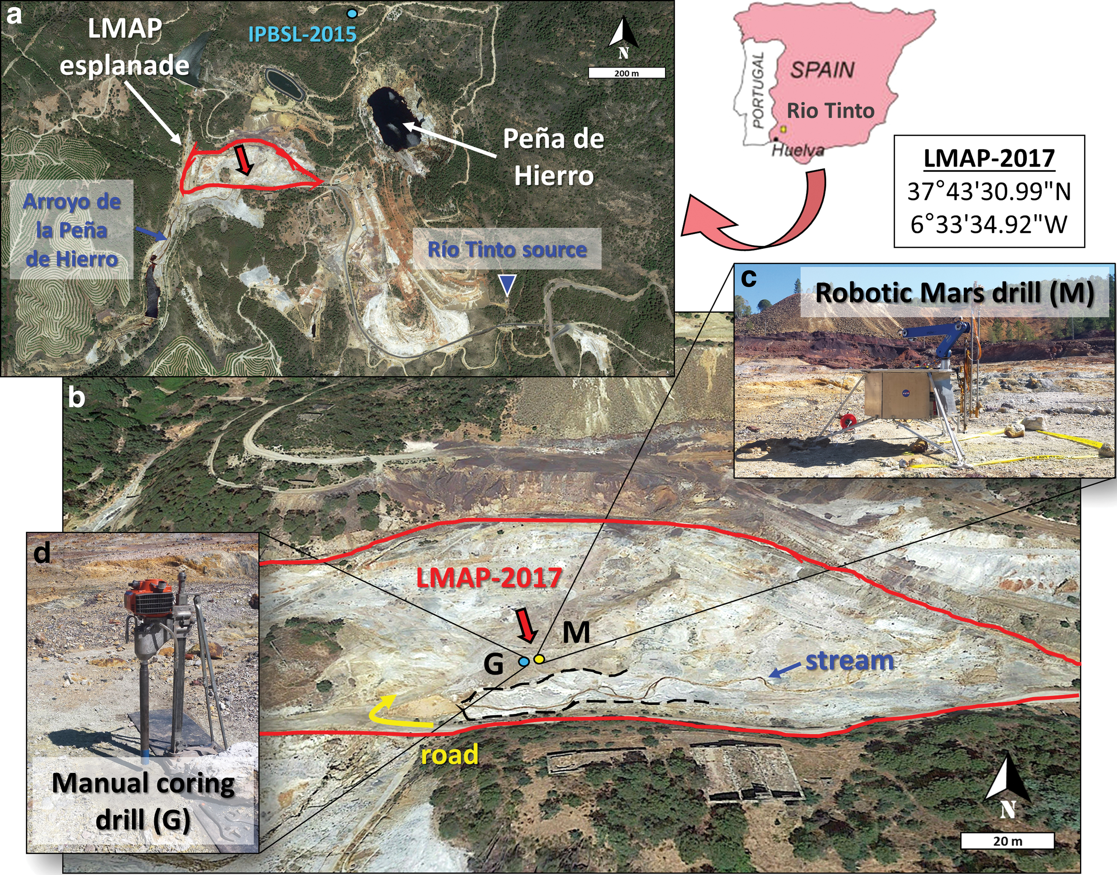
Site Drilling and study. Map of the study area in the Río Tinto basin (Southwestern Spain), with a regional map showing the location of the LMAP esplanade
Microbial life in Río Tinto is adapted to extreme conditions such as high acidity, abundance of heavy metals, and an Fe/S-based chemistry; acidophiles and chemolithotrophs are the major components of the microbial community. Eukaryotic microoorganisms contribute more than 60% of the Tinto basin biomass (López-Archilla et al., 2001), where a significant proportion of them are photosynthetic (mainly chlorophytes), whereas the prokaryotic diversity is mainly contributed (ca. 80%) by three bacterial genera (Leptospirillum spp., Acidithiobacillus ferroxidans, and Acidiphilium spp.) members of the iron cycle (González-Toril et al., 2003). As for the plants growing on the acidic soils of the Río Tinto basin (e.g., Pinus sp., Eucalyptus sp., Erica sp., Cistus ladanifer, or Taraxacum officinale), most of them use different strategies to overcome physiological problems associated with the extreme conditions of the habitat, such as accumulation of metals in plant tissues.
2.2. Sample collection
In June 2017, the Trident 1m-class planetary prototype drill was tested on an acidic site in Río Tinto, rich in sulfur-iron material, with stickiness properties that may be similar to those on Mars. Automated robotic drilling was conducted on the LMAP evaporitic esplanade (Fig. 1), adjacent to an acidic stream carrying little water as expected for the summer season and flowing about 350 m away into a larger stream called Arroyo de la Peña de Hierro (Fig. 1). The lander-mounted system (automated drill, robotic arm, and full-scale Phoenix-like lander deck) was deployed at the Mars-analog site (37°43′30.99″N and 6°33′34.92″W) (Fig. 1c). The Trident drill developed by Honeybee Robotics Spacecraft Mechanisms Corporation (Brooklyn, New York) is a 15 kg, rotary-percussive and fully autonomous robotic drill rated for lunar temperatures, with its own AI software executive (Glass et al., 2014). The drill power consumption was 30–40 W, 200 W max during 5–10-min drilling sequences. Drilling was conducted by using a bite-sampling approach, where samples were captured in 10–20 cm intervals to simulate a martian drilling scenario (Zacny et al., 2013). All pieces involved in the drilling campaign were initially autoclaved in the laboratory and then sterilized once deployed in the field. Iterative drill and scoop cleaning with organic solvents (acetone, dichloromethane, and methanol) was performed before each new hole was drilled to avoid human-sourced or cross contamination.
The surface to drill was previously scraped with a solvent-cleaned (dichloromethane and methanol) metal brush and stainless-steel spatula. Subsurface samples (cuttings) were automatically acquired from the drilling profile (i.e., robotic Mars drill or “M”) at every 20-cm depth (surface—20, 20–40, 40–60, 60–80, and 80–100 cm) and autonomously transferred by the robotic arm to sterile polypropylene jars for offline analysis. In parallel, a second borehole profile (i.e., ground-truth or “G”) was drilled ∼2 m away from M down to 2-m depth with a CARDI EN 400, a manual drill (with a 3 kW gas-powdered motor, and 85-mm diameter commercial off-the-shelf diamond-impregnated coring drill bits and rods) for manual validation. G samples were taken from the manual coring drill at different depth intervals (i.e., 10–20, 35–40, 50–60, 75–80, 90–95, 150–155, and 180–188 cm), covering different stratigraphic layers or interphases according to the lithological reconstruction (Fig. 2a).
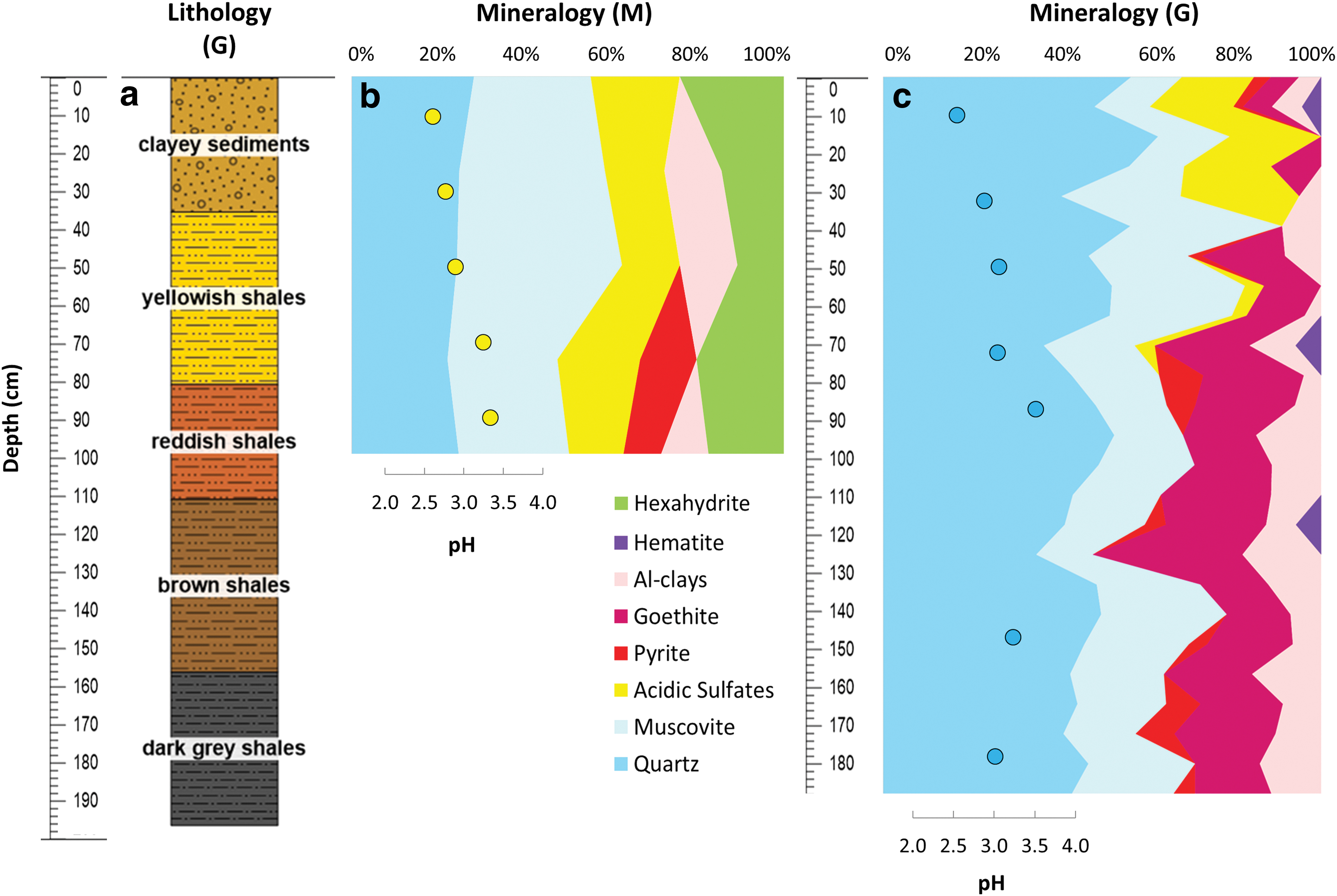
Stratigraphic column at the LMAP-2017 site, with the lithostratigraphic units reconstructed de visu on the manual coring drill (G)
Physical splitting and subsample handling were conducted wearing nitrile gloves and using solvent-cleaned stainless-steel material (spatulas and scoops). A total of 12 discrete samples of robotic Mars drill cuttings (n = 5; 30–70 g each) and manual coring drill subsamples (n = 7 of 200–300 g each) were collected and stored cold (∼4°C) in the field and during their transport to the laboratory 7 days later. Once in the laboratory, all samples were frozen to −20°C and freeze-dried before geochemical and biochemical analysis. All freeze-dried M and G samples were powdered (mortar and pestle) and homogenized before taking aliquots for the different biogeochemical analyses.
2.3. Bulk geochemistry analysis
The mineralogical composition of the M drill and G drill samples was measured by using an Olympus Terra X-ray analyzer. The Terra is a field portable X-ray diffraction/X-ray fluorescence instrument based on technology developed for the CheMin instrument on the Mars Science Laboratory rover (Sarrazin et al., 2005; Blake et al., 2012). The bulk sample is ground with a mortar and pestle and filtered to less than 150 microns; then, 15 mg is placed in an acoustically vibrated chamber that presents the instrument optics with multifarious orientations of the crystalline structure. This results in an X-ray diffraction pattern that is free of the problematic preferred-orientation effects. The angular range is 5–50° 2θ with diffraction resolution of 0.25–0.30° 2θ FWHM.
Anions and low-molecular-weight organic acids were measured by ion chromatography (IC) in the water-extractable phase of the M and G samples. For this analysis, 2 g of sample was sonicated (3 × 1 min cycles), diluted in 10 mL of deionized water, and filtered through a 22 μm GF/F. The supernatants were collected and loaded into a Metrohm 861 Advanced compact ion chromatographer (Metrohm AG, Herisau, Switzerland) undiluted or at dilution values, depending on ion concentrations. For all the anions, the column Metrosep A supp 7–250 was used with 3.6 mM sodium carbonate (NaCO3) as eluent. The pH of the water solutions was measured with a pH meter (WTW, GmbH & Co. KG, Weilheim, Germany) after 24 h of solution stabilization. More details of the IC analysis are fully described in Sánchez-García et al. (2018).
Stable isotopic composition of the bulk organic carbon (δ13C) and total nitrogen (TN) (δ 15N) were measured on the robotic Mars drill and manual coring drill samples with isotope-ratio mass spectrometry (IRMS), following USGS methods (Révész et al., 2012). Briefly, about 2 g of the subsurface samples was homogenized by grinding with a corundum mortar and pestle. To remove carbonates, HCl was added to the samples, let equilibrate for 24 h, and adjusted to neutral pH with ultrapure water. The residue was then dried (50°C) for 72 h; checked for a final, constant weight; and finally analyzed by IRMS (MAT 253; Thermo Fisher Scientific). The δ13C and δ 15N ratios were reported in the standard per mil notation by using three certified standards (USGS41, IAEA-600, and USGS40) with an analytical precision of 0.1‰. The content of total organic carbon (TOC % of dry weight [dw]) and TN (% dw) was measured with an elemental analyzer (HT Flash; Thermo Fisher Scientific) during the stable isotope measurements.
2.4. Lipid extraction, fractionation, and analysis
Lipids were extracted from the M and G samples with a method described in detail by Sánchez-García et al. (2019). Briefly, between 10 and 25 g of sample was extracted in a Soxhlet apparatus with a mixture of dichloromethane/methanol (DCM:MeOH, 3:1, v/v) during 24 h, after addition of three internal standards (tetracosane-D50, myristic acid-D27, 2-hexadecanol). After concentration to ∼2 mL and removal of elemental sulfur, the total lipid extracts (TLE) were separated into three fractions according to their different polarity (nonpolar, polar, and acidic). First, the TLE was passed through a Bond-Elut column (bond phase NH2, 500 mg, 40 μm particle size), where the neutral and acidic fractions were obtained by eluting with DCM:2-propanol (2:1, v/v) and subsequently acetic acid (2%) in diethyl ether, respectively. The neutral fraction was further separated into nonpolar and polar fractions by using an Al2O3 column (0.5 g of activated, 0.05–0.15-mm particle size Al2O3 in a Pasteur pipe), and eluting with hexane/DCM (9:1, v/v) and subsequently DCM/methanol (1:1, v/v), respectively. The acidic and polar fractions were trans-esterified (BF3 in methanol) and tri-methylsilylated (N,O-bis [trimethylsilyl] trifuoroacetamide [BSTFA]), respectively, before their analysis as fatty acid methyl esters (FAMEs) and tri-methyl silyl alkanols by gas chromatography–mass spectrometry (GC-MS).
The three lipid fractions were analyzed by GC-MS using a 6850 GC system coupled to a 5975 VL MSD with a triple axis detector (Agilent Technologies) operating with electron ionization at 70 eV and scanning from m/z 50 to 650. The analytes were injected (1 μL) and separated on a HP-5MS column (30 m × 0.25 mm i.d. × 0.25 μm film thickness) by using He as a carrier gas at 1.1 mL min−1. The oven temperature was programmed from 50°C to 130°C at 20°C min−1 and then to 300°C at 6°C min−1 (held 20 min) for the nonpolar fraction (i.e., hydrocarbons). For the polar (i.e., alkanols and sterols) and acidic (i.e., fatty acids) fractions, the oven temperature was programmed from 70°C to 130°C at 20°C min−1 and to 300°C at 10°C min−1 (held 10 min for the acidic or 15 min for the polar fractions). The injector temperature was 290°C, the transfer line was 300°C, and the MS source was 240°C.
Compound identification was conducted by comparing mass spectra and/or reference materials on mass-to-charge ratios of 57 (n-alkanes and isoprenoids), m/z = 74 (n-fatty acids as FAMEs), and m/z = 75 (n-alkanols and sterols). For compound quantification we employed external calibration curves of n-alkanes (C10–C40), n-FAME (i.e., FAMEs, C8–C24), n-alkanols (C10, C14, C18, and C20), and branched isoprenoids (2,6,10-trimethyl-docosane, crocetane, pristane, phytane, squalane, and squalene), all from Sigma Aldrich. The recoveries of the internal standards were measured to average 72% ± 23%.
2.5. DNA extraction, polymerase chain reaction amplification, and DNA sequencing
Total genomic DNA was extracted from the M and G samples by using the commercial kit PowerMax Soil DNA Isolation Kit (MO BIO Laboratories, Inc.), following the manufacturer's instructions with a 1-h (room temperature) enlargement of the lysis step. Polymerase chain reaction (PCR) amplification was then carried out on bacterial 16S rDNA V3–V4 gene (using the primer pairs 341-F/805-R, Herlemann et al., 2011) following Warren-Rhodes et al. (2018) specifications. Illumina MiSeq sequencing (Illumina, Inc., San Diego, CA) was then employed to construct a paired-end amplicon library.
Amplicon reads were processed with MOTHUR software v.1.40.0 (Schloss et al., 2009), by using a custom script based on MiSeq SOP (Kozich et al., 2013). Briefly, the pipeline consisted of several reads-trimming steps based on both quality and length (>400 bp) criteria. After trimming, sequence reads were clustered into operational taxonomic units (OTUs) at 97% of sequence similarity level. Even sequencing depth—corresponding to the lesser number of sequences found within the samples, that is, 63,736—was obtained by independent rarifying of datasets by random selection.
OTU representative sequences were then compared against the RDP database (RDP reference files v.16; release 11) (Cole et al., 2014) for taxonomic affinities assignment. Those OTU sequences reported as “cyanobacteria/chloroplast” were further assigned a taxonomic identity by comparing them against nr/nt (NBCI), EMBL, Greengenes, and SILVA databases for more precise cyanobacteria taxonomic identification. The sequences assigned to “mitochondria” or “chloroplast” were removed from further analyses. Community parameters, such as phylogenetic richness (S, total number of OTUs) and Shannon diversity index (H′), were calculated on the samples by using R package “vegan” (Oksanen et al., 2017). The same statistical package was also employed to perform a correspondence analysis (CA) for microbial classes and bulk geochemistry parameters (standardized and log-normalized).
2.6. Multiplex fluorescent sandwich microarray immunoassay
Powdered subsurface M and G samples were analyzed by a fluorescent sandwich microarray immunoassay (FSMI) with the LDChip immunosensor (i.e., LDChip) (Rivas et al., 2008; Parro et al., 2008; 2011). The LDChip is a shotgun antibody microarray produced for the simultaneous detection of potential microbial biomarkers from environmental samples (Parro et al., 2018; Sanchez-García et al., 2019) and/or for detecting possible traces of life in the field of the planetary exploration (Blanco et al., 2017; Moreno-Paz et al., 2018) as part of the SOLID instrument concept (Parro et al., 2008, 2011).
The LDChip is composed of 200 polyclonal antibodies produced against a wide range of immunogens: small organic molecules, peptides and proteins, and other biopolymers (exopolysaccharides, lipopolysaccharides), spores, or whole cells (bacteria and archaea) from extant or well-preserved remains of extinct life (Rivas et al., 2008; Sanchez-García et al., 2018). The antibodies used in this work are described in detail elsewhere (Sanchez-García et al., 2018, and in table S1 supplementary materials in Sánchez-García et al., 2019). In addition, bovine serum albumin, protein printing buffer, and preimmune sera were used as negative controls. To build the microarray, the immunoglobulin (IgG) fraction of each antibody was purified with protein-A by using the PURE1A kit (Sigma Aldrich Quimica S.L.) and printed onto microscope slides in a triplicate spot-pattern. Antibodies were titrated, fluorescently labeled with Alexa 647, and used to perform the FSMI as reported in Rivas et al. (2008).
In this study, Río Tinto subsurface samples were analyzed in the field with the LDChip immunosensor as previously described (Rivas et al., 2008; Parro et al., 2011; Blanco et al., 2012). Briefly, 0.5 g of each sample was suspended in 2 mL of TBSTRR buffer (0.4 M Tris-HCl pH 8, 0.3 M NaCl, 0.1% Tween 20), homogenized with a handheld ultrasonicator to extract the organic matter, and finally filtered through a 5-μm filter. A volume of 50 μL of each filtrate was used for the FSMI as a multianalyte-containing sample in the multiarray analysis cassette as previously described (Rivas et al., 2008; Blanco et al., 2017; Moreno-Paz et al., 2018). After a washing step, 50 μL of the mixture of 200 alexa-647 labeled antibodies was incubated in each chamber and then scanned in the GenePix 4100A scanner and the resulting images were analyzed and quantified by the GenePix Pro 7.0 Software (Molecular Devices, Sunnyvale, CA). The fluorescence intensity (F) of positive antigen-antibody reactions was calculated as reported by Rivas et al. (2011). To avoid false positives in the FSMI, fluorescent signal intensities for each antibody were considered positives when they had intensity at least 2.5 times the background level.
3. Results
3.1. Profiling the geochemistry of 1-m depth robotic drill in Río Tinto sediments
A simulated Mars drill (M) down to 1 m was performed with a rotary-percussive and fully autonomous robotic drill prototype on iron/sulfur-rich sediments in an evaporitic material about 10 m apart from the river stream (Fig. 1). As a ground-truth experiment, a second drill (G) was carried out ∼2 m far from M, by using a commercial, manual drilling and coring system (Section 2). The M drill rendered samples with a few tens of grams (20–70 g) of material, whereas G allowed us to collect hundreds of grams (Table 1) so that the mass required for multiple analyses at the different depths was not a limitation.
Concentration of Inorganic and Organic Anions (μg·g− 1) in the Subsurface Samples Along the Robotic Mars (M) and Manual Coring (G) Drills
n.d. = not detected.
The X-ray diffraction analysis revealed a subsurface mineralogy primarily composed of quartz and muscovite (Fig. 2). The relative abundance of both mineral species varied between the robotic M drill and manual coring G drill profiles, with muscovite being dominant (25–38%) along M (Fig. 2b) and quartz (35–63%) along G (Fig. 2c). Acidic sulfate minerals, including jarosite, natrojarosite, and copiapite, were similarly abundant throughout the M drill (13–21%) and in the upper layers (down to 80 cm) of the G profile (3–27%). Both M and G set of samples contained a ubiquitous comparable proportion (11–13% versus 4–18%, respectively) of aluminous clays (i.e., chlorite, vermiculite, montmorillonite, and kaolinite). In contrast, pyrite was only patchy throughout the two profiles and hematite was only detected in the G drill. Hexahydrite and goethite were distributed ubiquitously throughout the M (11–24%) and G (6–34%) profiles, respectively (Fig. 2).
The IC analysis detected the presence of diverse soluble inorganic and organic anions (Table 1). Sulfate was the most abundant anion among both the M (56–78 μg·g−1) and G (35–48 μg·g−1) samples. Chloride and fluoride were similarly abundant throughout the two drills (Fig. 3b, c) whereas bromide, nitrate, and phosphate were only present at low concentrations (≤0.215 μg·g−1) in a few depths of either the M or G profiles (Table 1). Formate showed concentrations ranging from 0.031 to 0.044 μg·g−1 in the M samples, and from 0 to 0.085 μg·g−1 in the G series (Fig. 3d). Acetate was detected to be ubiquitous throughout the M profile (0.022–0.041 μg·g−1), but only patchy (0–0.047 μg·g−1) along G (Fig. 3e).
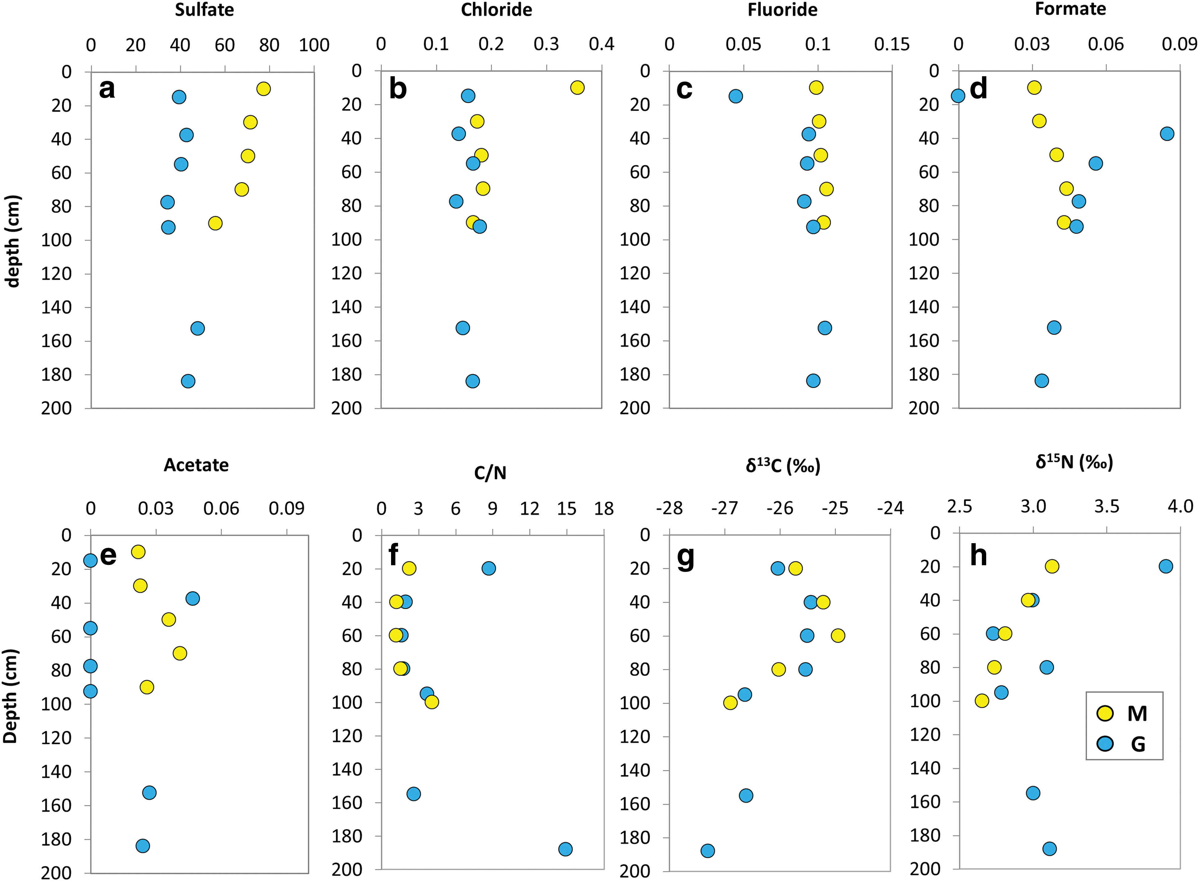
Depth distribution of bulk (elemental, molecular, and isotopic) geochemical variables in the Mars robotic drill (M, yellow) and manual coring drill (G, blue) profiles. Scatterplots showing the concentration (μg·g−1) of inorganic
The TOC content ranged from 0.12% to 0.38% (wt/wt) of dw among M and from 0.12% to 1.3% (wt/wt) among G (Table 2). The TN content ranged from 0.067% to 0.10% (wt/wt) in G and from 0.078% to 0.10% (wt/wt) in M, resulting in generally similar ratios of TOC to TN ratios (i.e., C/N) in both the M and G profiles (Fig. 3f). The carbon isotopic ratio (δ13C) varied from −27.3‰ to −25.4‰ in G and from −26.9‰ to −24.9‰ in M, whereas the nitrogen isotopic ratio from 2.7‰ to 3.9‰ in G and from 2.7‰ to 3.1‰ in M (Fig. 3g, h).
Concentration (ng·g− 1 of Dry Weight) of Lipid Biomarkers and Bulk Elemental and Stable Isotopic Composition of Organic Matter in the Subsurface Samples Along the Robotic Mars (M) and Manual Coring (G) Drills
Ratio of TOC over TN.
ACL of C10–C40 n-alkanes; C6–C33 n-fatty acids; and C10–C30 n-alkanols. ACL i-n = ∑(i·Xi +…+ n·Xn)/∑Xi +…+ Xn), where X is concentration (van Dongen et al., 2008).
CPI, CPI i-n = ½ Σ(Xi+Xi+2+…+Xn)/Σ(Xi−1+Xi+1+…+Xn−1) + ½Σ(Xi+Xi+2+…+Xn)/Σ(Xi+1+Xi+3+…+Xn+1), where X is concentration (van Dongen et al., 2008).
Ratio of odd, HMW alkanes (C27, C29, and C31) over even, LMW alkanes (C16, C18, and C20).
Sum of iso- and anteiso- n-fatty acids (C11–C29).
9-Hexadecenoic acid (measured as hexadec-9-enoate that is a fatty acid methyl ester).
9/11-Octadecenoic acid (measured as octadec-9/11-enoate).
9,12-Octadecenoic acid (measured as octadec-9,12-enoate).
24-Methylcholest-5-en-3β-ol.
24-Ethylcholest-5,22-dien-3β-ol.
24-Ethylcholest-5-en-3β-ol.
ACL = average chain length; CPI = carbon preference index; dw = dry weight; HMW = high molecular weight; LMW = low molecular weight; TN = total nitrogen; TOC = total organic carbon.
3.2. Lipid biomarker profiles
The GC-MS analysis of TLE from M and G set of samples yielded molecular biomarkers within the families of n-alkanes, isoprenoids, FAMEs, n-alkanols, and sterols. Straight chain fatty acids (a.k.a. normal or n-fatty acids) of 6 to 33 carbons were measured at concentrations from 129 to 1320 ng·g−1 of dw (Table 2). They showed average chain length (ACL) ranging from 14 to 26. n-Fatty acids with one [e.g., C16:1 (ω7) or C18:1 (ω7/9)] or two [C18:2 (ω6,9)] unsaturations were also detected (Table 2). Branched fatty acids with iso- and anteiso configuration (i-/a-) were detected between C11 and C29 at concentrations from 9 to 223 ng·g−1 dw (Fig. 4a), with predominance of the i/a-C15 and i/a-C17 compounds (Fig. 4b). Fatty acids with two carboxyl groups (i.e., dioic or dicarboxylic acids) from 6 to 30 carbons were also found at concentrations ranging from 0.7 to 173 ng·g−1 dw (Table 1 and Fig. 4c).
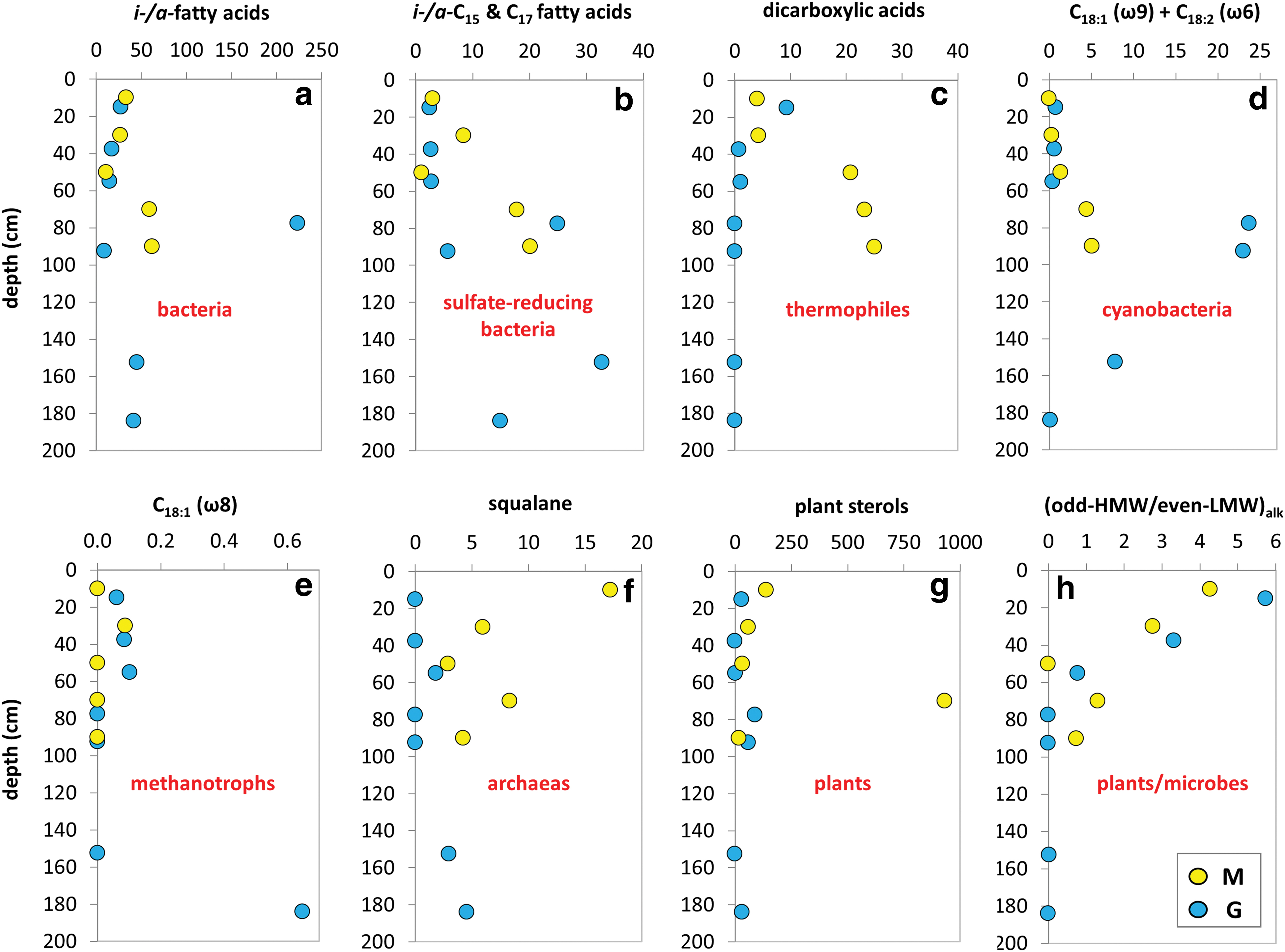
Depth distribution of lipid biomarkers along the Mars robotic drill (M, yellow) and manual coring drill (G, blue) profiles. Concentration (ng·g−1dw) of lipids, biomarkers of bacteria as iso-/anteiso-fatty acids of C11–C29
Straight chain alkanols (i.e., n-alkanols) of ACL ranging from 17 to 32 were measured in the m/z = 75 ion at concentrations from 150 to 21,363 ng·g−1 dw, together with terrestrial sterols (Goad and Akihisa, 1997) such as campesterol, stigmasterol, and β-sitosterol (3.6–1194 ng·g−1 dw; Table 2 and Fig. 4g).
Straight chain alkanes (n-alkanes) with between 10 and 40 carbons were measured at concentrations from 144 to 9164 ng·g−1 dw (Table 2). They exhibited molecular distribution with dominance of the high-molecular-weight (HMW) homologs that produced ACL between 22 and 32 (Table 2). The carbon preference index of the n-alkanes was generally lower than one in the two profiles, except at the 0–20 cm (M and G) and 75–80 cm (G) depth intervals. The ratios of vegetal, odd HMW (i.e., C27, C29, and C31) over microbial, low-molecular-weight (LMW) n-alkanes (Eglinton and Hamilton, 1967), both odd LMW (C17, C19, and C21) and even LMW (C16, C18, and C20), were generally larger than the ones throughout both drills down to the 80–100-cm interval (Fig. 4h). Isoprenoids such as pristane, phytane, and squalane were detected in the same ion as the n-alkanes (i.e., m/z = 74) at total concentrations ranging from 0.037 to 18 ng·g−1 dw (Table 2).
3.3. Prokaryotic diversity by DNA sequencing
Total DNA was extracted from both set of samples, used for PCR amplification of the 16S rRNA gene, sequencing, and bioinformatic analysis. The results indicated that the bacterial OTUs adscriptions along the drills were largely represented by Proteobacteria, Firmicutes, and Actinobacteria phyla, together accounting for 85% and 93% of the total bacterial reads in the M and G drills, respectively. Along the M drill, Actinobacteria and Clostridia classes were more abundant (21% of bacterial reads in these samples) in the upper layers, whereas Bacilli and Gammaproteobacteria were more abundant with depth (21%) (Fig. 5a). Other classes such as Alpha- and Betaproteobacteria represented only 1.9% and 3.3% of the sequences found at the M drill. The microbial community in the G drill was rather dominated by Alphaproteobacteria (48%), with minor presence of the other classes mentioned earlier (Fig. 5b). In both the M and G drills, Cytophagia, Bacteroidia, Deltaproteobacteria, Deinococci, and Cyanobacteria classes were found at minor proportion (<1%) (Fig. 5).
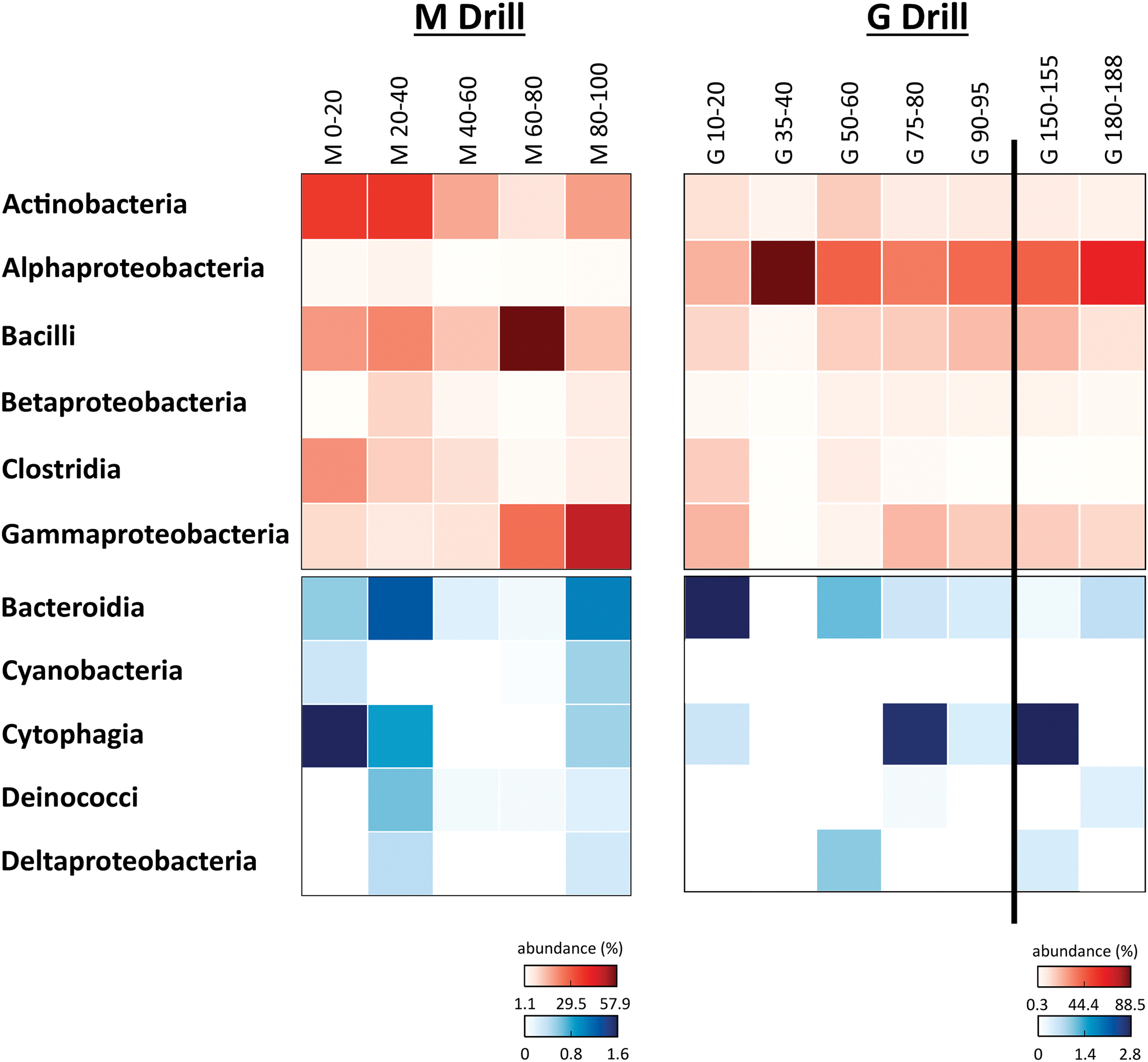
Bacterial DNA diversity. Heat maps showing the relative abundance (number of sequences at the class level) along the Mars robotic drill (M) and manual coring drill (G) profiles. Only bacterial classes accounting for >0.5% of total number of sequences are plotted. Both heat maps are split into two to better show the relative abundance of the less represented classes (blue scale). In both the red and blue scales, white color indicates absence of sequences (please notice the different % of abundance in each heat map). Color images are available online.
Within the described classes, the most abundant family along the M drill was Staphylococcaceae (Bacillales order, Bacilli class; 3–16% of bacterial reads). This family showed greater abundance in the upper sections of M, along with unclassified families belonging to the orders Actinomycetales (Actinobacteria; 2–15%) and Clostridiales (Firmicutes; 2–12%) (Fig. 6). In contrast, the families Oceanospirillaceae (Oceanospirillales, Gammaproteobacteria; 0.003–8%) and Vibrionaceae (Vibrionales, Gammaproteobacteria; 0.02–37%) were relatively more abundant at deeper layers. Neisseriaceae (Neisseriales, Betaproteobacteria; 0.6–5% of bacterial reads) and Moraxallaceae (Pseudomonadales, Gammaproteobacteria; 1–4%) were families less abundantly represented in M (Fig. 6).
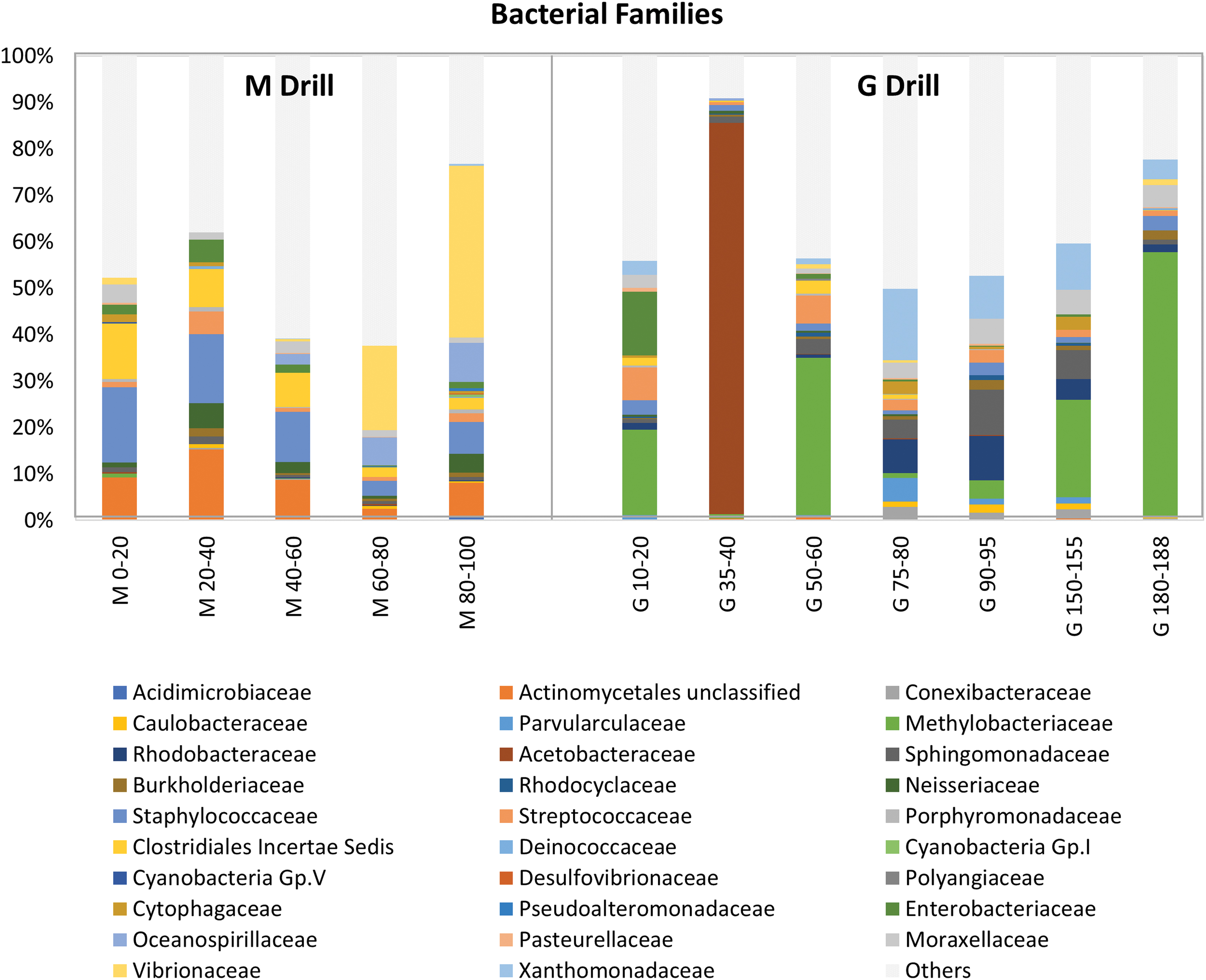
Comparison of bacterial community composition along the robotic Mars drill (M) versus manual coring drill (G) profiles. Relative abundance (number of sequences) of bacterial families along the M and G profiles. Only the most abundant family within each order is represented. Less abundant families are grouped in the “others” category (light gray bars). Color images are available online.
The bacterial community at the G drill showed a slightly different structure, with a widespread distribution of Methylobacteriaceae (Rhizobiales, Alphaprotebacteria; 0.9–57%) that showed its highest abundance at the deepest section (Fig. 6). A comparable widespread distribution, but accounting for a much lower number of bacterial reads, was that of Xanthomonadaceae (Xanthomonadales, Gammaproteobacteria; 0–15%), Sphingomonadaceae (Sphingomonadales, Alphaproteobacteria; 0.9–10%), Rhodobacteraceae (Rhodobacterales, Alphaproteobacteria; 0.002–10%), Moraxallaceae (Pseudomonadales, Gammaproteobacteria; 0.002–5%), and Streptococcaceae (Lactobacillales, Bacilli; 0.6–7%). From those, Streptococcaeae was more abundant in the upper layers of the G drill, whereas Xanthomonadaceae, Sphingomonadaceae, Rhodobacteraceae, and Moraxallaceae were preferentially distributed at depth (Fig. 6). Of special interest was the particularly high abundance (84% of sequences) of the family Acetobacteraceae (Rhodospirillales, Alphaproteobacteria) in almost exclusively the 35–40-cm depth interval in G (Fig. 6).
The CA of bacterial classes and mineralogy-geochemistry (Fig. 7) showed that all samples belonging to the same drill clustered together along the CA1 axis (explaining 59.8% of variance). Only the most surficial sample from the G drill (10–20-cm depth) was positioned near the M samples. CA2 accounted for 22.4% of total variance explained by the analysis, and it grouped the samples according to a depth pattern (Fig. 7). Most of the bacterial classes were located close to the ordination center, with Alphaproteobacteria clearly clustering along with the G samples, Clostridia and Actinobacteria located close to M samples from the upper layers, and Gammaproteobacteria and Bacilli located close to deep M layers. Samples from the M profile showed higher influence from geochemical features such as δ13C, chloride, or pyrite, muscovite and acidic sulfates; whereas those from G were rather affected by the amount of quartz, goethite, TOC, or aluminous clays.
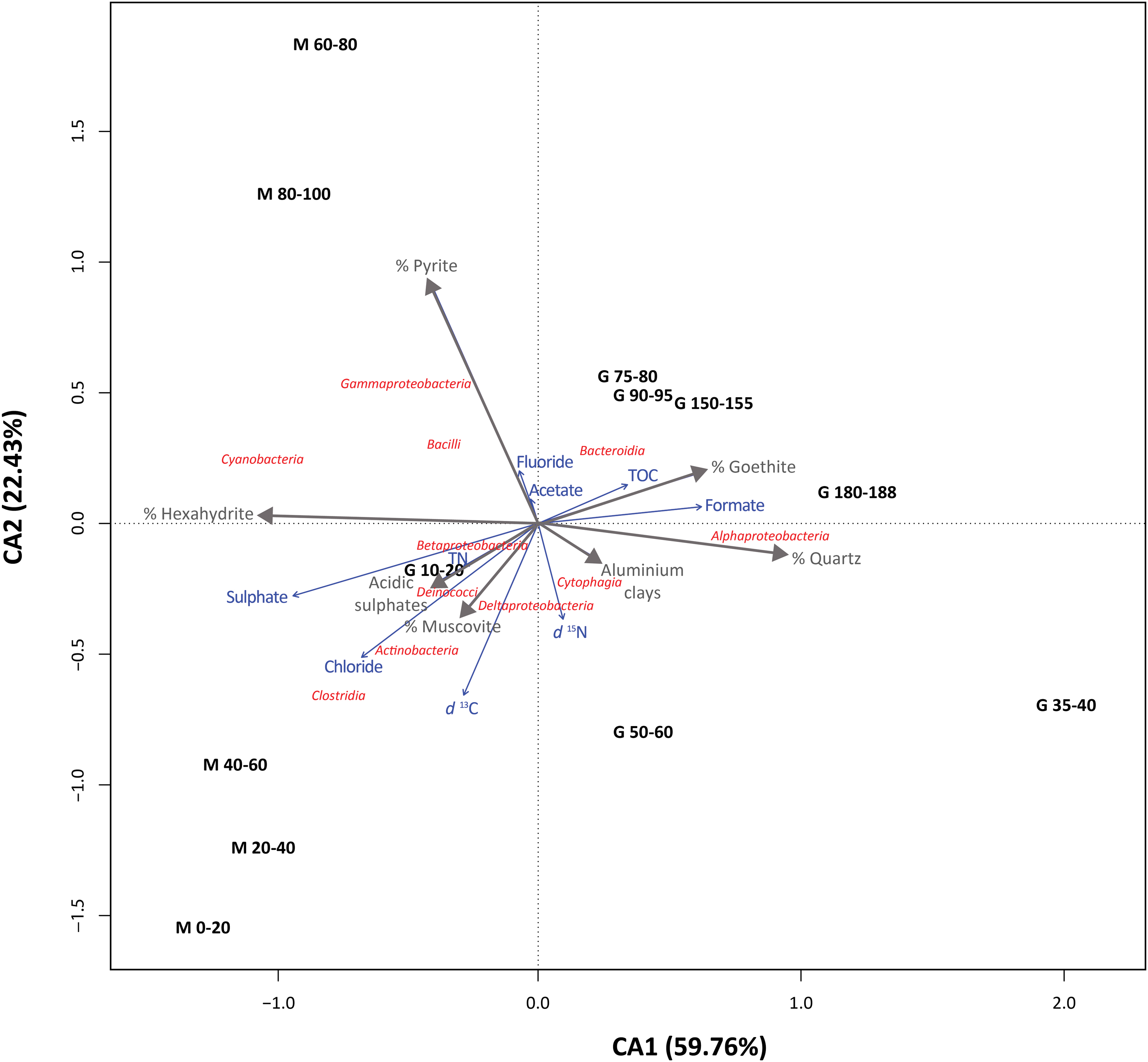
Single CA of bacterial classes (red) from different sampling depths (black) along the robotic drill (M) and manual coring drill (G) profiles with mineralogical (gray) and geochemical variables (blue). Only bacterial classes accounting for >0.5% of total number of sequences are plotted. In total, CA1 and CA2 explained 82.19% of the dataset's variance. The closer the clustering of microbial groups and/or mineralogical/geochemical variables to a sampling profile and depth, the more characteristic these groups are at that site and the more explained by the local mineralogy/geochemistry they are. Distance among sampling sites depicts compositional differences between them, and arrow length of the participation of each geochemical/mineralogical variable in explaining the variance. CA, correspondence analysis. Color images are available online.
Samples from the M drill contained a higher number of OTUs (i.e., S ranging from 699 to 939) than those from the G drill (S = 330–638). This resulted in the Shannon diversity index (H′) ranging from 2.14 to 3.76 in M and from 1.07 to 3.90 in G. In both drills, the bacterial community richness (S) decreased from the surface to 20–40 cm depth in G, or 40–60 cm in M, showing a maximum at 40–60 cm in G or 60–80 cm in M (Fig. 8a). The microbial diversity (H′) displayed a general decrease along the M drill, with an upturn in the deepest interval (Fig. 8b). Overall, the H′ index varied little throughout the G drill, except for the 35–40- and 180–188-cm depths showing lower values.
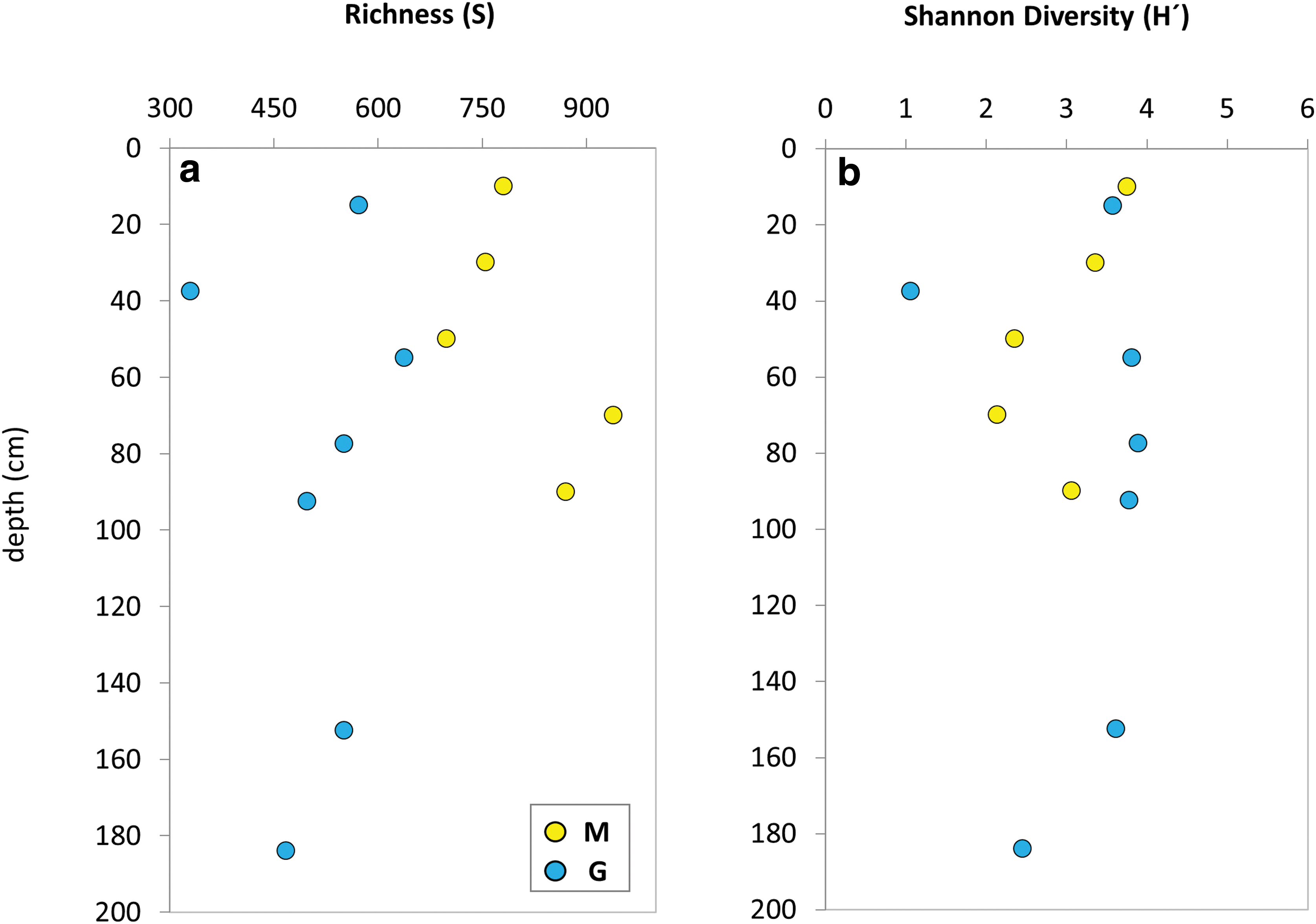
Estimation of microbial richness
3.4. Microbial markers profiling with an LDChip immunoassay
Up to 0.5 g of each sample from the two drills was processed and analyzed for detecting microbial markers by FSMIs (Section 2). The fluorescence intensity for each antibody spot in the LDChip microarray was quantified, corrected by the background and blank control, and represented as a heat map showing the relative fluorescence intensity of the positive immunodetections by the LDChip (Fig. 9).
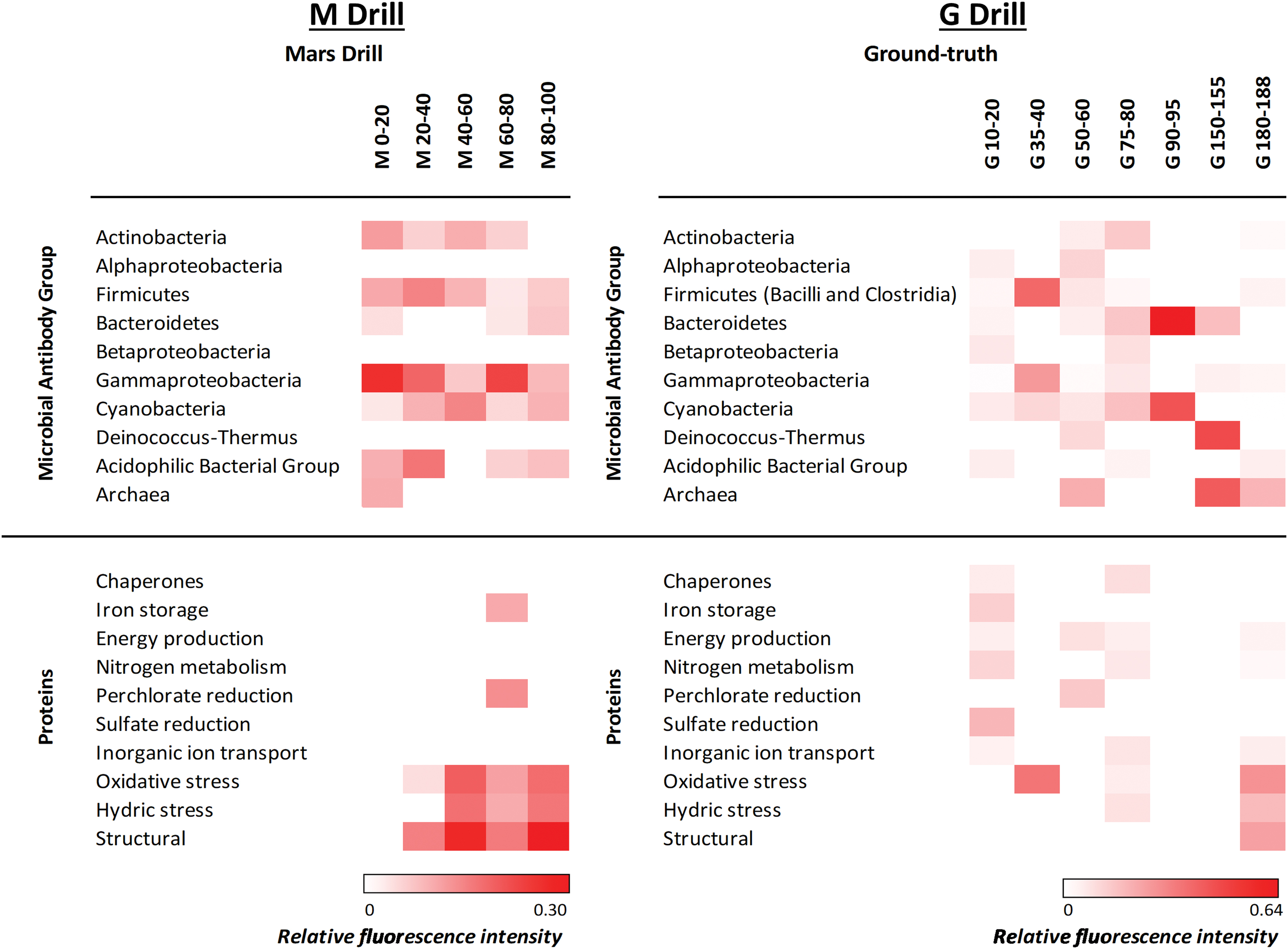
Heat map representing relative fluorescence signals obtained in the M and G samples with fluorescent sandwich microarray immunoassay in the LDCHip microarray immunosensor. Antibodies were grouped in different categories corresponding to main prokaryotic groups and proteins involved in several potential metabolisms. Antibodies printed in the microarray are described in Section 2. Proteins detected with the LDChip in this work are as follows: (1) chaperones: HscA and GroEL; (2) iron storage protein BFR (bacterioferritin); (3) energy production: Bacteriorodopsin, RRO (rubredoxin), NADH Deshidrogenase quinone, and OmcS (C-type cytochrome); (4) nitrogen metabolism: NifD, NifS, NirS (nitrite reductase), and NRA (nitrate reductase); (5) perchlorate reduction: perchlorate reductase; (6) sulfate reduction: DsrA (dissimilatory sulfite reductase subunit A); (7) inorganic ion transport: ModA and K+ tranporter; (8) oxidative stress: CcdA (cytochrome c-type biogenesis), PhcA2 (phycocyanin alpha-subunit), DhnA2 (fructose-bisphosphate aldolase), and PufM2 (photosynthetic reaction center M subunit); (9) hydric stress: SodA and SodF (superoxide dismutases) and WshR (water stress protein); and (10) structural: FtsZ (cell division protein). Relative fluorescence intensity of each category was calculated as the average of the fluorescence intensity for each antibody in three replicate samples and considering no redundant positive immunodetections for each category. Relative fluorescence intensity was plotted in a color gradient scale ranging from 0 to 1 (white represented values below the limit of detection and red values for the maximum fluorescence intensity obtained for each drill profile). LDChip, life detector chip. Color images are available online.
In the M drill, the LDChip showed positive immunodetections of Gammaproteobacteria (mainly Acidithiobacillus spp, Psicrobacter sp., and Halothiobacillus sp.), Firmicutes (mainly Bacillus subtilis spores), Actinobacteria (both mycelium and spores of Streptomyces), and Cyanobacteria (Anabaena spp.). Also, positive signals from Bacteroidetes and cellular and exopolysaccharide extracts from Río Tinto (streams and biofilms; González-Toríl et al., 2003), here named as “acidophilic bacterial group,” were also observed at certain depths (Fig. 9a). This group was dominated by acidophilic iron oxidizers such as Leptospirillum spp. (Nitrospirae), Acidithiobacillus spp. (Gammaproteobacteria), and Acidimicrobium spp. (Actinobacteria). In addition, the sulfide-oxidizing bacterium Sulfobacillus acidophilus (Firmicutes) was also detected throughout the M drill. Archaeal markers (Halorubrum spp., and Pyroccoccus spp.) were detected only in the most-shallow sample of the M drill.
In the G drill, the LDChip showed a patchy distribution with no particular pattern with depth, except Bacteroidetes, Cyanobacteria (Anabaena sp. and Microcystis sp.), Deinococcus-Thermus, and Archaea (Halorubrum spp., and Pyroccoccus spp.) that were slightly more abundant in deeper samples (Fig. 9b). The “acidophilic bacterial group” was only detected in some G samples always at a lower fluorescence signal intensity than in the M drill (Fig. 9). Finally, iron reducers such as Acidocella sp. and Acidiphilium sp. (Alphaproteobacteria), the anaerobic sulfate-reducing bacterium Desulfosporinus meridiei (Firmicutes), and the chlorate-reducer Ideonella spp. (Betaproteobacteria) were also identified by the LDChip overall in the upper layers of the G drill.
The LDChip also showed positive immunodetection of proteins involved in relevant metabolic processes such as hydric stress (water stress-resistance protein WshR or superoxide dismutase proteins SodA and sodF) or oxidative stress (antioxidant protein PhcA2, which is phycocianin α-chain from Nostoc), mostly in the M drill (Fig. 9a). Other proteins involved in septation and sporulation processes in Streptomyces and Bacillus such as the FtsZ (Beall and Lutkenhaus, 1991) or CcdA (Schiott and Hederstedt, 2000) were detected in M from 20-cm depth. In the G drill, the proteins related to oxidative and hydric stress (SodA, sodF, and WhsR) were only detected at 75–80- and mostly 180–188-cm-depth intervals (Fig. 9b). Other proteins detected and irregularly distributed in G were chaperone-like proteins (i.e., HscA and GroEL) or those involved in energy metabolism (i.e., NADH dehydrogenase quinone, bacteriorhodopsin, rubredoxin, and cytochromes), nitrogen fixation (i.e., NifD and NifS of Leptospirillum sp.), nitrate reduction (i.e., nitrate reductase, or NRA of Micrococcus spp.), and nitrite reduction (nitrite reductase or NirS protein) (Fig. 9b).
4. Discussion
4.1. Multianalytical biomarker profiling along a Mars simulated drill
The analysis of different molecular biomarkers revealed a ubiquitous presence of microbial biomass throughout the 1m-depth M drill profile. On one hand, there was a generalized detection of i-/a- fatty acids (Fig. 4a) typically associated to bacterial sources (Kaneda, 1991), consistent with low C/N ratios (Fig. 3f). Organic matter with C/N ratios between 4 and 10 (here ≤4.1) reflect microbial activity in contrast to plant-derived material typically showing C/N ≥ 20 (Meyers, 1994), owing to the abundance of cellulose in vascular plants and its absence in microorganisms, together with the remineralization of carbon and immobilization of nitrogenous material by microbes (Sollins et al., 1984; Schubert and Calvert, 2001). On the other hand, immunodetections of structural proteins involved in cell division and septation such as FtsZ were also generally detected throughout the M drill, except for the most surficial layer (Fig. 9a). The DNA sequencing indicated that the ubiquitous microbiology was dominated by members of the Actinobacteria, Bacilli, Clostridia, and Gammaproteobacteria classes (Fig. 5).
Microbial biomass signals showed certain distribution patterns with depth along the M drill. For instance, microorganisms commonly found in soil and decaying organic matter (Actinomycetales) were more abundantly measured down to 60-cm depth, along with Staphylococcaceae and spore-forming unclassified Clostridiales (Fig. 6a), both (facultative and strict, respectively) anaerobes. This was consistent with the immunodetection of spore-forming Firmicutes (Bacillus) and Actinobacteria (Streptomyces) with LDChip, mostly down to 60-cm depth (Fig. 9a). At the same time, the immunodetection of proteins involved in mechanisms of resistance to desiccation (SodA, sodF, and WshR) revealed a hydric stress in the deeper half of the M profile, more or less mirroring the distribution of proteins involved in reducing damage caused by oxidative stress (Ccda, PhcA2, DhnA2, and PufM2). Archaeal biomarkers, measured as both lipid proxies of halophilic archaea (i.e., squalane; ten Haven et al., 1988) and positive immunodetections against Halorubrum spp. and Pyroccoccus spp., were preferentially found in the upper M layers (Figs. 4f and 8a, respectively).
In addition, microbes particularly resistant to heavy metals such as Moraxellaceae were also more abundant in upper layers (Fig. 6a), coinciding with immunodetection of Gammaproteobacteria (including Moraxellaceae) involved in sulfur oxidation (i.e., Acidithiobacillus spp, Psicrobacter sp., and Halothiobacillus sp.) (Fig. 9a). In contrast, heterotrophic Vibronaceae, also resistant to heavy metals, facultative anaerobes capable of doing fermentation, were relatively more abundant in samples below 60 cm, similar to Oceanospirillaceae (Fig. 6a).
Lipid biomarkers such as C15 and C17 i-/a- fatty acids related with sulfate-reducing bacteria (Kaneda, 1991) (Fig. 4b) or dicarboxylic acids (Fig. 4c) elsewhere described as proxies of thermophiles (Carballeira et al., 1997) were increasingly detected with depth (Fig. 4b, c). Other source-specific lipid proxies such as the mono-unsaturated C18:1 (ω8) fatty acid (methanotrophic biosignatures; Boschker and Middleburg, 2002 and references therein) did not show a particular depth pattern (Fig. 4e).
Despite the acidic pH conditions (Fig. 1b), low but generalized presence of cyanobacterial markers was consistently detected by DNA sequencing (ca. 1%), LDChip (e.g., Anabaena spp.), and lipid biomarkers (C18:1 [ω9], and C18:2 [ω6] fatty acids; Cohen et al., 1995; Allen et al., 2010) along the M drill. So far, Cyanobacteria have not been found in acidophilic environments. Some of us have recently reported viable cyanobacteria in rocky cores from a 607m-depth borehole 500 m far northeast from our sampling site (IPBSL-2015 in Fig. 1), but at pH values higher than 6 (Puente-Sánchez et al., 2018). The unexpected presence of these endolithic and hypolithic cyanobacteria in the dark deep subsurface of the Río Tinto area was explained by specific adaptations to environmental and nutritional stress, such as the use of molecular hydrogen as energy source (Puente-Sánchez et al., 2018). This possibility can also be considered in this study, where Cyanobacteria could occupy specific high pH (≥4–5) microniches, which is not unreasonable considering the mineralogical (Fig. 2b, c) and geochemical (Fig. 3a) variability observed in barely 2 m of horizontal distance between the M and G drills. Also, inputs of allochthone organic matter from upper, surrounding less acid terrains would provide a suitable habitat for Cyanobacteria, such as those northward of the LMAP esplanade (e.g., Puente-Sánchez et al., 2018). In addition, the generalized presence of impermeable clay-rich and shale layers together with the hydric stress inferred from LDChip signals of hydric stress proteins (Fig. 9a) could contribute toward creating those high pH microniches for cyanobacterial strains.
This microbial community observed is consistent with a biomass δ13C and δ15N composition (Fig. 3g, h) reflecting carbon fixation pathways related to the Calvin cycle or reductive acetyl-CoA pathway (Hayes, 2001), and nitrogen metabolisms linked to N2 fixation via nitrogenase, organic N assimilation, and/or NH4 + production from organic matter decomposition (δ15N values from 0‰ to 6‰; Robinson, 2001). Microorganisms fixing carbon through the Calvin cycle (e.g., Cyanobacteria, other photosynthetic bacteria, and some archaea) produce biomass δ13C values relative to CO2 ranging from −18‰ to −30‰ (Guy et al., 1993), whereas those using the reductive acetyl-CoA pathway (variety of anaerobic, nonphotosynthetic bacteria and archaea) result in δ13C values from −23‰ to −44‰ (Preuβ et al., 1989). In our drilled samples, different members of the Firmicutes, Alpha, Beta, and Gammaproteobacteria phyla are potential users of either of the two carbon fixation pathways; whereas members of Cyanobacteria and Alphaproteobacteria (Rhizobiales), as well as algae and/or plants are capable of nitrogen fixation.
Compared with the M drill samples, the microbial community in G was rather dominated by families involved in methylotrophic metabolism (Methylobacteriacea), acidophilic microorganisms that use O2 and Fe+3 as electron acceptors (Acetobacteraceae), heavy metal-resistant microorganisms (Rhodocyclaceae, Moraxellacea, and Enterobacteriaceae), or nitrite reducers (Xanthomonadaceae) (Fig. 6b). In contrast to the M community, no particular depth pattern was observed in the distribution of the microbial community along the G drill.
Overall, the difference between the M and G holes was remarkable for the lipid (Fig. 4), DNA (Figs. 5 and 6), and antibody biomarkers (Fig. 9). The microbial community in M was, overall, richer and less diverse than that along the G drill (Fig. 8). The depth pattern described earlier for the microbial community in M appeared to be somehow influenced by mineralogical and geochemical features, as the subsurface samples of the robotic drill were clustered in the CA according to their depth (Fig. 7). On the one hand, muscovite and acidic sulfates together with the biomass δ13C and chloride content seemed to be major drivers of the microbial community at the upper layers, largely represented by members of the Actinobacteria and Clostridia classes. On the other hand, the presence of pyrite was a key factor for explaining the microbial composition of the deeper communities in M, dominated by Gammaproteobacteria. In contrast, the microbial community in G, mostly represented by Alphaproteobacteria, did not follow a clear depth pattern (Fig. 7). Yet, certain differentiation was observed between deep samples (from 75 to 188 cm) largely influenced by the amount of goethite, formate, or TOC, and those from upper layers (from 35 to 60 cm depth) more affected by factors such as the proportion of quartz or the δ15N ratio (Fig. 7a). In summary, we postulate that the mineralogy and bulk geochemistry influenced habitability in this particular Río Tinto shallow subsurface Mars analog, where a number of biomarkers displayed distribution patterns along the depth profiles.
4.2. Different factors influencing the multianalytical microbial detection
The present multianalytical study produced some diverging results responding to different factors that deserve a detailed discussion according to their nature. Overall, result discrepancies were attributable to (i) different detection techniques (i.e., analysis of lipid material, DNA sequencing, or immunoassays), (ii) different sampling systems (i.e., robotic drill versus manual vibro-coring), and (iii) spatial variability of mineralogy and geochemistry.
The first factor attributes such discrepancies to the analytical constraints of each technique. On one hand, each of the three techniques applied here for detecting biomarkers has targets of different composition (i.e., free organic-soluble lipids versus DNA sequences versus diverse antigens), biological specificity, and resistance to degradation. Lipids are structural components of cell membranes, ubiquitous in all organisms and, thus, of less taxonomic specificity. As a counterpart, they are among the most recalcitrant organic biomarkers, with hydrocarbon skeletons being capable of resisting degradation for up to billions of years (Brocks and Summons, 2003). In contrast, genetic (i.e., nucleic acid sequences of DNA) and immunological (i.e., peptidic and nonpeptidic epitopes from microorganisms and biological polymers pursued by the LDChip) biomarkers are among the most labile biomolecules. The differential specificity and preservation potential of lipids, DNA, or antigens influence the detection capacity of each approach, thus leading us to expect results that are not necessarily comparable from a quantitative and even qualitative perspective. This explains the different level of taxonomic detail obtained from the lipids (detecting only certain general groups) versus the DNA or LDChip (detecting phylogenetic groups from phyla to family) results.
In addition, some biomarkers (lipids) show lower source specificity than others (DNA or antibodies) because of their nature (i.e., structural components of cell membranes generally present in most phylogenetic groups), thus offering a relatively less exclusive source diagnosis. That is the case with, for instance, squalane, dicarboxylic acids, or different polyunsaturated C18 fatty acids that, despite occurring potentially in other organisms even in most (e.g., squalane), are likely to derive mostly from archaea (squalane; Brocks and Summons, 2003), cyanobacteria (C18:1 [ω9] and C18:2 [ω6]; Willers et al., 2015 and references therein), or simply have been described just in certain groups to date (e.g., dicarboxylic acids on thermophiles, Carballeira et al., 1997; or C18:1 [ω8] on methanotrophs, e.g., Bowman et al., 1991 or Bodelier et al., 2009). All this may explain, to some extent, the lack of agreement in the detection of certain groups (e.g., archaea) by DNA sequencing, LDChip, and lipid biomarkers. Besides, a low abundance of archaeal biomass relative to other biological sources (e.g., bacteria, algae or plants) reduces the detection capability of its DNA by sequencing techniques. In contrast, the higher sensitivity of the immunological LDChip or the greater resistance to degradation of lipid remnants allows the detection of archaeal biomass even at low concentrations (Figs. 4f and 9).
Beyond being a limiting factor, handling such heterogeneous results has a positive aspect, that is, the complementary information the three biomarker types provide on biological terms, with DNA affording high taxonomic specificity from resisting genetic material, the LDChip providing high sensitivity on the detection of a defined number of microorganisms and proteins (i.e., 200 antibodies), and the lipid biomarkers offering the best estimation of the existing biomass with distinction of general sources (i.e., prokaryotic vs. eukaryotic, aquatic vs. terrestrial, or a number of source-specific microbes). On the other hand, each detection approach belongs to a different type of analytical method, where the LDChip is a microarray immunoassay interrogating a panel with a finite number of polyclonal antibodies (i.e., close method); whereas the other two approaches are able to detect any existing genetic (DNA) or structural (lipid) material (i.e., open methods). This difference explains the lack of detection by the LDChip of certain microbial groups that were detected by DNA sequencing (e.g., Alpha- and Betaproteobacteria, or Deinoccoci) in the M drill.
Finally, the size of analytical sample varies considerably from one to another approach (i.e., 10–25 g of subsurface sample for lipid extraction, 10 g for DNA extraction, and 0.5 g for the LDChip immunoassay), which certainly affected how representative the analytical sample is of the whole field sample (i.e., material from each depth interval).
The second factor refers to the different approach followed to collect samples from the Río Tinto-analog subsurface. On one hand, the Trident drill autonomously accessed the terrain to 100-cm depth for acquiring small subsurface samples (i.e., ≤70 g) in the form of cuttings from 20-cm-depth intervals. On the other hand, about 100–200 g of subsurface material was sampled manually at different depth intervals (covering different visually determined color layers; Fig. 2a) from the 200-cm-deep G drill acquired with a manual vibro-corer. The different (collection) sample size and slightly different depth interval covered by each sampling technique, as well as the mixing (M) versus not-mixing (G) procedures, may explain part of the divergences observed between the biomarker patterns in the M versus G profiles, such as those of lipid proxies (e.g., archaeal squalane; Fig. 4f), phylogenetic groups (e.g., Proteobacteria or Cyanobacteria; Figs. 5 and 9), or metabolic processes (Fig. 9).
Complementary with the latter, a third and last diverging factor is the spatial geochemical and mineralogical heterogeneity across the sampled terrain that may also contribute to explaining the different biomarker profiles between the M and G drills. In about 2 m of distance, mineralogical (e.g., pyrite and hexahydrite; Fig. 1b, c) and geochemical features such as the concentration of sulfate, formate, or acetate (Fig. 3a, d, and e, respectively) varied considerably from the M to the G drills. Small-scale heterogeneity is an important factor for being considered in any drilling analysis both on Earth and on Mars, with sample homogenization being a difficulty in robotic missions. In fact, in a comparable distance (i.e., ∼140 cm), differences in the bulk geochemistry (calcium oxide and calcium sulfates) were observed between the Cumberland and John Klein holes, the first two martian drills analyzed by the Mars Science Laboratory in the apparently uniform sedimentary Sheepbed Mudstone, an ancient lacustrine environment in Yellowknife Bay (Jackson et al., 2016).
The spatial variability is a relevant aspect to be taken into account in life detection missions, as it likely plays a role in defining environmental differences at a microscale (i.e., niches) that certainly influences the preferential development of certain microorganisms or the differential preservation of their remnants. Consequently, small-scale heterogeneity may have an important impact on the drilling and sampling strategies in missions such as IceBreaker (McKay et al., 2013).
Altogether, factors related to analytical constraints, biological specificity, chemical resistance, sampling approach, and environmental heterogeneity contributed to producing heterogeneous results hardly comparable from a quantitative perspective, but rather complementary in the forensic information they supply from biomarkers of different scope (lipids, DNA sequences, or immunodetections).
5. Conclusions
The autonomous lander-mounted drilling system successfully demonstrated fully robotic and intelligent sample acquisition and transfer for biomarker detection in the Río Tinto-Mars analog site. The Trident drill mounted on a NASA Phoenix/InSight-like mockup platform provided subsurface samples that allowed for a multianalytical investigation of microbial diversity at a high level of detail (structural, phylogenetic, and metabolic). The parallel manual sampling and analysis of lipid, genetic, and immunological biomarkers demonstrated feasibility and fidelity of the automated biomarker-searching approach. A diverse subsurface microbial community was found to be ubiquitous, with a certain association of microbial biomarkers with abiotic variables such as mineralogy, bulk geochemistry, and/or local scarcity of water.
The spatial heterogeneity of such abiotic variables at a local microscale, thus, raised the relevance of considering several drilling sites for achieving a good coverage and local representativity of the target area. Still, sampling different lithologies may be also paramount for increasing the chances of detecting life biomarkers. Assuming the complexity of deciding on the best sampling targets and considering the limited number of drills that could be taken in a given life detection mission, a compromise must be reached between lithological variability and spatial coverage of a priority target area. This is an important aspect for future Mars astrobiology missions, where the window of success is narrow and detecting low concentrations (if any) of potential biosignatures is complicated.
Detecting residual biosignatures in extreme environments such as the martian subsurface may prove highly challenging owing to the combination of expected low biomass, existence of mineral and rocky refugia in a variable mineralogy and geochemistry, and a resulting patchy biomarker distribution. Assuming that any potential biomarker on Mars is expected to be scarce and diffusedly scattered throughout the martian subsurface (even forming micro-niches), covering the maximum extension possible (both in depth and horizontal distance) is key for increasing the chances of detection.
Aiming for the best radiation-preserved (perhaps organic) material, future ESA ExoMars rover mission plans to drill down to 2 m, and the IceBreaker mission concept plans to go down to 1m depth. We report here a successful demonstration of autonomous drilling down to 1m depth as a proof-of-concept study. The drill apparatus employed in this study has demonstrated that subsurface biosignatures spanning a wide range of compositional nature, preservation potential, and taxonomic specificity can be recovered from an iron-rich Mars analog site. Although genetic biosignatures (i.e., DNA sequences) may not be the primary method used to search for traces of life on Mars, their use in this study corroborated and complemented the information obtained from other methods currently used or foreseen in future missions (i.e., lipid GC-MS, and SOLID-LDChip). The high preservation potential of lipid biomarkers, the high sensitivity of the LDChip for detecting biopolymers, and the complementary information provided by both techniques make them fundamental components for IceBreaker mission payload for searching for molecular evidence of life in the martian ice-cemented subsurface.
Footnotes
Author Disclosure Statement
No competing financial interests exist.
Funding Information
This work has been funded by the Spanish Ministry of Science, Innovation and Universities and Fondo Europeo de Desarrollo Regional (MICINN/FEDER) projects No. CGL2015-74254-JIN, ESP2015-69540-R, and RYC-2014-19446; the State Research Agency (AEI) Project no. MDM-2017-0737 Unidad de Excelencia “María de Maeztu”; and the NASA PSTAR project No. 13-MMAMA13-0007.