Sage Journals: Discover world-class research

Abstract

We present a catalog of spectra and geometric albedos, representative of the different types of solar system bodies, from 0.45 to 2.5 μm. We analyzed published calibrated, uncalibrated spectra, and albedos for solar system objects and derived a set of reference spectra and reference albedos for 19 objects that are representative of the diversity of bodies in our solar system. We also identified previously published data that appear contaminated. Our catalog provides a baseline for comparison of exoplanet observations to 19 bodies in our own solar system, which can assist in the prioritization of exoplanets for time intensive follow-up with next-generation extremely large telescopes and space-based direct observation missions. Using high- and low-resolution spectra of these solar system objects, we also derive colors for these bodies and explore how a color–color diagram could be used to initially distinguish between rocky, icy, and gaseous exoplanets. We explore how the colors of solar system analog bodies would change when orbiting different host stars. This catalog of solar system reference spectra and albedos is available for download through the Carl Sagan Institute.

1. Introduction

The first spectra of extrasolar planets have already been observed for gaseous bodies (e.g., Snellen et al., 2010; Kreidberg et al., 2014; Dyudina et al., 2016; Mesa et al., 2016; Sing et al., 2016). To aid in comparative planetology, exoplanet observations will require an accurate set of disk-integrated reference spectra and albedos of solar system objects. To establish this catalog for the solar system, we use disk-integrated spectra from several sources. We use uncalibrated and calibrated spectra as well as albedo when available from the literature to compile our reference catalog. About half of the spectra and albedos we derive in this article are based on uncalibrated observations obtained from the Tohoku-Hiroshima-Nagoya Planetary Spectral Library (THN-PSL) (Lundock et al., 2009), which provides a large coherent data set of uncalibrated data taken with the same telescope. Our analysis shows contamination of part of that data set, as discussed in Sections 2.1 and 2.2; therefore, we only include a subset of their data in our catalog (Section 4.3).

This article provides the first catalog of calibrated spectra (Fig. 1) and geometric albedos (Fig. 2) of 19 bodies in our solar system, representative of a wide range of object types: all 8 planets, 9 moons (representing, icy, rocky, and gaseous moons), and 2 dwarf planets (Ceres in the Asteroid belt and Pluto in the Kuiper belt). This catalog is available through the Carl Sagan Institute¹ to enable comparative planetology beyond our solar system.

FIG. 1.

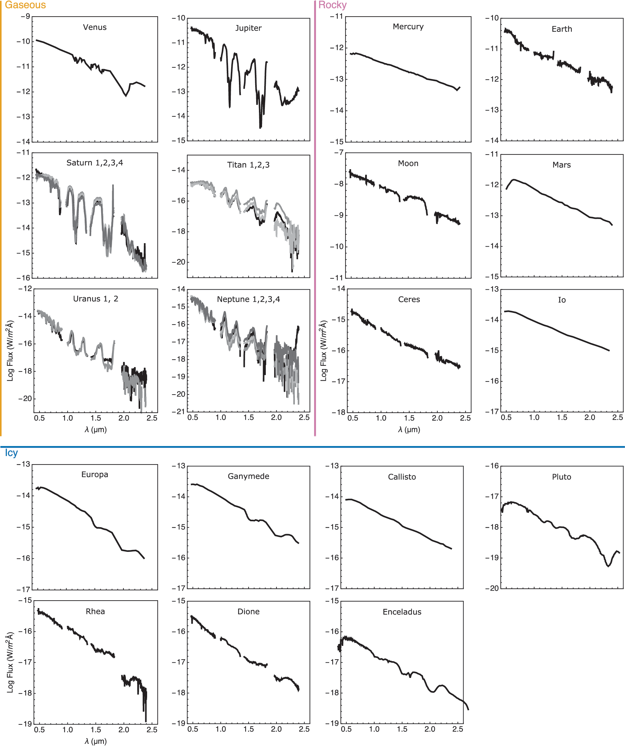
Spectra for 19 solar system bodies for Ceres, Dione, Earth, Jupiter, Moon, Neptune, Rhea, Saturn, Titan, Uranus (albedos calculated in this article based on uncalibrated data by Lundock et al., 2009), Callisto (Spencer, 1987), Enceladus (Filacchione et al., 2012), Europa (Spencer, 1987), Ganymede (Spencer, 1987), Io (Fanale et al., 1974), Mars (McCord and Westphal, 1971), Mercury (Mallama, 2017), Pluto (Protopapa et al., 2008; Lorenzi et al., 2016), and Venus (Meadows, 2006 [theoretical]; Pollack et al., 1978 [observation]). Items are arranged by body type then by distance from the Sun.

FIG. 2.

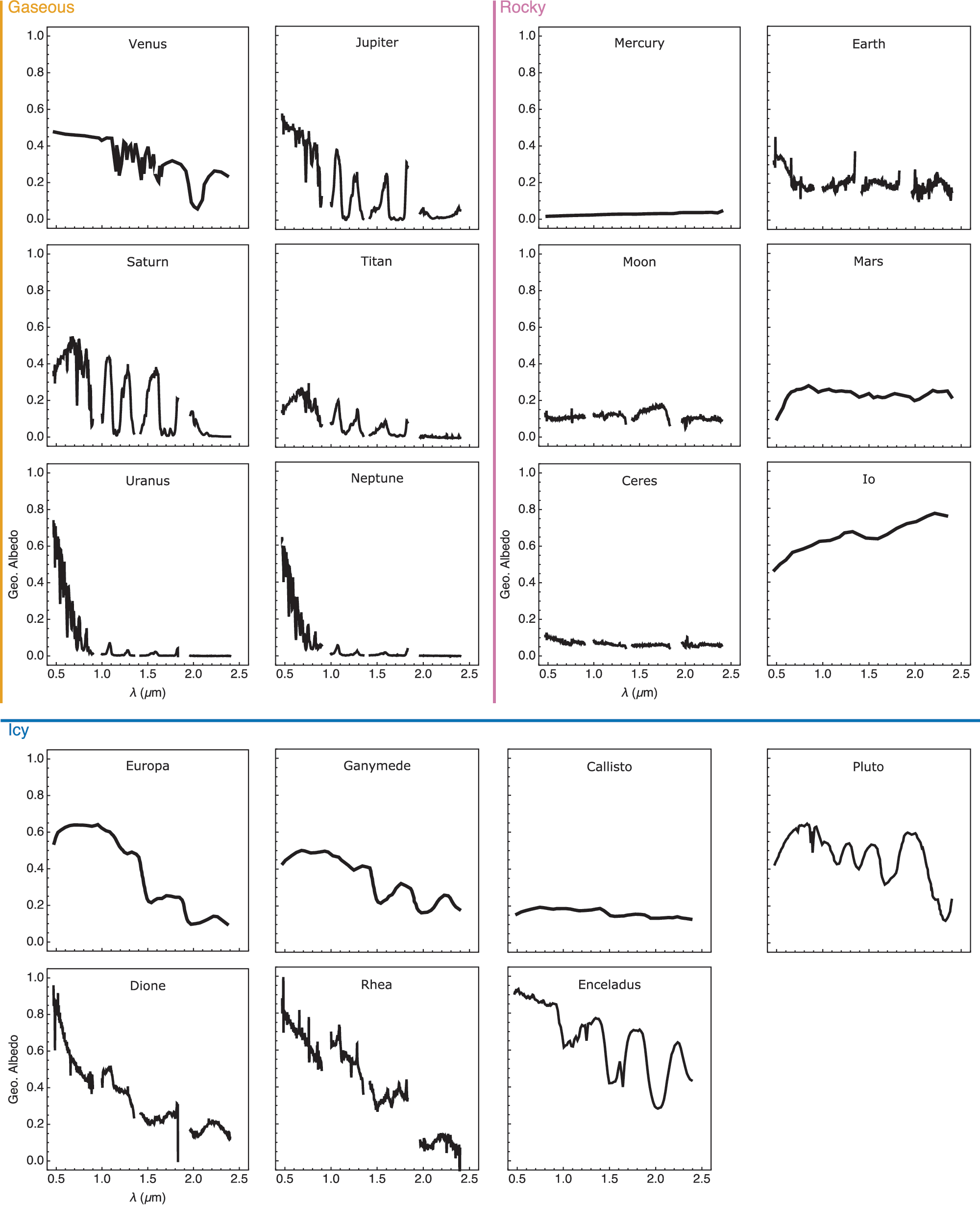
Geometric albedos for 19 solar system bodies for Ceres, Dione, Earth, Jupiter, Moon, Neptune, Rhea, Saturn, Titan, Uranus (albedos calculated in this article based on uncalibrated data by Lundock et al., 2009), Callisto (Spencer, 1987), Enceladus (Filacchione et al., 2012), Europa (Spencer, 1987), Ganymede (Spencer, 1987), Io (Fanale et al., 1974), Mars (McCord and Westphal, 1971), Mercury (Mallama, 2017), Pluto (Protopapa et al., 2008; Lorenzi et al., 2016), and Venus (Meadows, 2006 [theoretical]; Pollack et al., 1978 [observation]). Items are arranged by body type then by distance from the Sun.

Several teams have shown that photometric colors of planetary bodies can be used to initially distinguish between icy, rocky, and gaseous surface types (Traub, 2003; Lundock et al., 2009; Cahoy et al., 2010; Krissansen-Totton et al., 2016) and that models of habitable worlds lie in a certain color space (Traub, 2003; Hegde and Kaltenegger, 2013; Krissansen-Totton et al., 2016). We expand these earlier analyses from a smaller sample of solar system objects to 19 solar system bodies in our catalog, which represent the diversity of bodies in our solar system bodies. In addition, we explore the influences of spectral resolution on characterization of planets in a color–color diagram by creating low-resolution versions of our data. Using the derived albedos, we also explore how colors of analog planets would change if they were orbiting other host stars.

Section 2 of this article describes our methods to identify contamination in the THN-PSL data, derive calibrated spectra, albedos, and colors from the uncalibrated THN-PSL data, and show how we model the colors of the objects around the Sun and other host stars. Section 3 presents our results, Section 4 discusses our catalog, and Section 5 summarizes our findings.

2. Methods

We first discuss our analysis of the THN-PSL data and show how we identified contaminated data in detail, then discuss how we derived spectra and albedo from the uncontaminated data. Finally we discuss spectra and albedo from other data sources for our catalog.

2.1. Calibrating the spectra of solar system bodies from the THN-PSL

The THN-PSL is a collection of observations of 38 spectra for 18 solar system objects observed over the course of several months in 2008. The spectra of one of the objects, Callisto, were contaminated and could not be reobserved, whereas the spectrum for Pluto in the database is a composite spectrum of both Pluto and Charon. We analyzed the data for the 16 remaining solar system objects for additional contamination and found 6 apparently contaminated objects among them, leaving 10 objects in the database that do not appear contaminated. Their albedos are similar to published values in the literature for the wavelength range such data are available for. We show the derived albedos for both contaminated and uncontaminated data from the database in Fig. 3, compared with available values from the literature for these bodies.

FIG. 3.

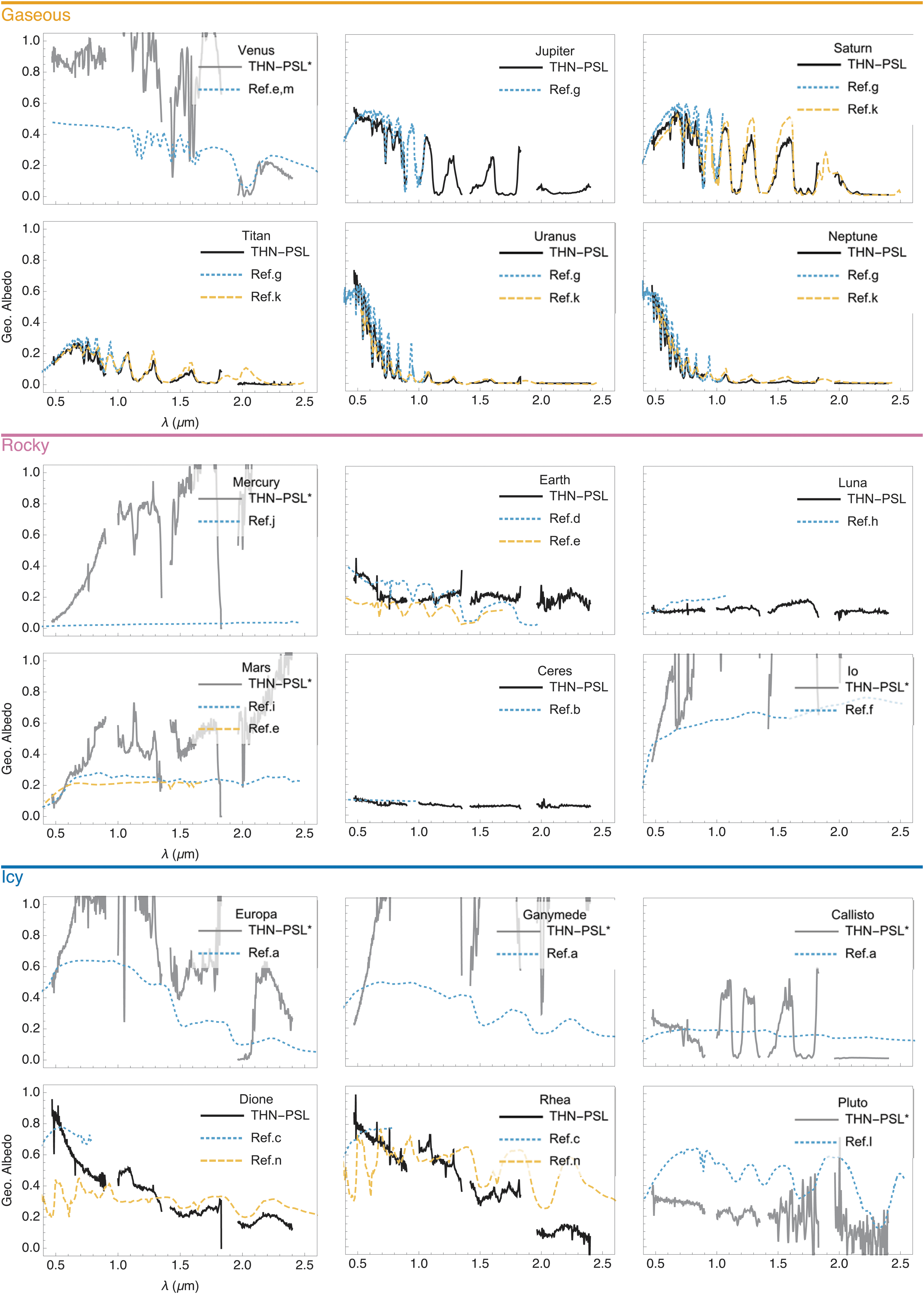
A comparison of geometric albedos for the solar system bodies in our catalog between published values and the albedo calculated from the THN-PSL data. THN-PSL data-based albedos are denoted with solid lines for uncontaminated data and with an asterisk and gray line if contaminated. References for comparison albedos: a (Spencer, 1987), b (Reddy et al., 2015), c (Noll et al., 1997), d (Kaltenegger et al., 2010), e (Meadows, 2006), f (Fanale et al., 1974), g (Karkoschka, 1998), h (Lane and Irvine, 1973), i (McCord and Westphal, 1971), j (Mallama, 2017), k (Fink and Larson, 1979), l (Protopapa et al., 2008; Lorenzi et al., 2016), m (Pollack et al., 1978), and n (Cassini VIMS—NASA PDS). Items are arranged by body type then by distance from the Sun. THN-PSL, Tohoku-Hiroshima-Nagoya Planetary Spectral Library.

The THN-PSL data were taken in 2008 using the TRISPEC instrument while on the Kanata Telescope at the Higashi-Hiroshima observatory. TRISPEC (Watanabe et al., 2005) splits light into one visible channel and two near-infrared channels, giving a wavelength range of 0.45–2.5 μm. The optical band covered 0.45–0.9 μm and had a resolution of \documentclass{aastex}\usepackage{amsbsy}\usepackage{amsfonts}\usepackage{amssymb}\usepackage{bm}\usepackage{mathrsfs}\usepackage{pifont}\usepackage{stmaryrd}\usepackage{textcomp}\usepackage{portland, xspace}\usepackage{amsmath, amsxtra}\usepackage{upgreek}\pagestyle{empty}\DeclareMathSizes{10}{9}{7}{6}\begin{document}$$R = \lambda / \Delta \lambda = 138$$ \end{document} . The first infrared (IR) channel has a coverage from 0.9 to 1.85 μm and had a resolution of \documentclass{aastex}\usepackage{amsbsy}\usepackage{amsfonts}\usepackage{amssymb}\usepackage{bm}\usepackage{mathrsfs}\usepackage{pifont}\usepackage{stmaryrd}\usepackage{textcomp}\usepackage{portland, xspace}\usepackage{amsmath, amsxtra}\usepackage{upgreek}\pagestyle{empty}\DeclareMathSizes{10}{9}{7}{6}\begin{document}$$R = 142$$ \end{document} . The second IR channel has a coverage from 1.85 to 2.5 μm and had a resolution of \documentclass{aastex}\usepackage{amsbsy}\usepackage{amsfonts}\usepackage{amssymb}\usepackage{bm}\usepackage{mathrsfs}\usepackage{pifont}\usepackage{stmaryrd}\usepackage{textcomp}\usepackage{portland, xspace}\usepackage{amsmath, amsxtra}\usepackage{upgreek}\pagestyle{empty}\DeclareMathSizes{10}{9}{7}{6}\begin{document}$$R = 360$$ \end{document} . Note that the slit subtends 4.5 arcseconds by 7 arcmin, meaning that spectra for larger bodies such as Saturn and Jupiter were not disk integrated (Section 4). As discussed in the original article, all spectra are unreliable <0.47 μm and between 0.9 and 1.0 μm from a dichroic coating problem with the beam splitters. Near 1.4 and 1.8 μm, Earth's water absorption degrades the quality and >2.4 μm thermal contamination is an issue. These wavelength regions are grayed out in all relevant figures in our article but do not influence our color analysis, due to the choice of filters. The raw data available for download include all data points.

The THN-PSL article discusses several initial observations of moons that were contaminated with light from their host planet, rendering their spectra inaccurate (080505 Callisto, 081125 Dione, 080506 Io, and 080506 Rhea). These objects (with the exception of Callisto) were observed again and the extra light was removed in a different manner to more accurately correct the spectra (Lundock et al., 2009). Callisto was not reobserved and, therefore, the THN-PSL Calisto data remained contaminated (Fig. 3).

The fluxes of the published THN-PSL observations were not calibrated but arbitrary normalized to the value of 1 at 0.7 μm. This makes the data set generally useful to compare the colors of the uncontaminated objects, as shown in the original article, but limits the data's usefulness as reference for extrasolar planet observations because geometric albedos can only be derived from calibrated spectra. The conversion factors used in the original publication were not available (Ramsey Lundock, pers. comm.).

However, in addition to the V magnitude, the THN-PSL gives the color differences: V-R, R-I, R-J, J-K, and H-Ks for each observation, providing the R, I, and J magnitudes. Therefore, we used the published V, R, I, and J magnitudes to derive the conversion factor for each spectrum to match the published color magnitudes and to calibrate the THN-PSL observations.

We define the conversion factor k such that \documentclass{aastex}\usepackage{amsbsy}\usepackage{amsfonts}\usepackage{amssymb}\usepackage{bm}\usepackage{mathrsfs}\usepackage{pifont}\usepackage{stmaryrd}\usepackage{textcomp}\usepackage{portland, xspace}\usepackage{amsmath, amsxtra}\usepackage{upgreek}\pagestyle{empty}\DeclareMathSizes{10}{9}{7}{6}\begin{document}$$k{f_{norm}} = \;f { \rm{ \;}} ;$$ \end{document} , where \documentclass{aastex}\usepackage{amsbsy}\usepackage{amsfonts}\usepackage{amssymb}\usepackage{bm}\usepackage{mathrsfs}\usepackage{pifont}\usepackage{stmaryrd}\usepackage{textcomp}\usepackage{portland, xspace}\usepackage{amsmath, amsxtra}\usepackage{upgreek}\pagestyle{empty}\DeclareMathSizes{10}{9}{7}{6}\begin{document}$${f_{norm}}$$ \end{document} and f are the normalized and absolute spectra, respectively. Adapting the method outlined in Fukugita et al. (1995), the magnitude in a single band using the filter response, V, and the spectrum of Vega, \documentclass{aastex}\usepackage{amsbsy}\usepackage{amsfonts}\usepackage{amssymb}\usepackage{bm}\usepackage{mathrsfs}\usepackage{pifont}\usepackage{stmaryrd}\usepackage{textcomp}\usepackage{portland, xspace}\usepackage{amsmath, amsxtra}\usepackage{upgreek}\pagestyle{empty}\DeclareMathSizes{10}{9}{7}{6}\begin{document}$${f_{vega}}$$ \end{document} , are given by Equation 1. The spectrum of Vega (Bohlin, 2014)² and the filter responses are the same as in the THN-PSL publication and shown in Figs. 4 and 5, respectively. The filters we used are V (Johnson and Morgan, 1953); R and I (Cousins, 1976; Bessell, 1979); and J, H, K, and Ks (Tokunaga et al., 2002). Since the THN-PSL article recorded the V, R, I, and J color magnitudes for each object, we derive the conversion factor to obtain each magnitude and average them to obtain k. For example, we substitute \documentclass{aastex}\usepackage{amsbsy}\usepackage{amsfonts}\usepackage{amssymb}\usepackage{bm}\usepackage{mathrsfs}\usepackage{pifont}\usepackage{stmaryrd}\usepackage{textcomp}\usepackage{portland, xspace}\usepackage{amsmath, amsxtra}\usepackage{upgreek}\pagestyle{empty}\DeclareMathSizes{10}{9}{7}{6}\begin{document}$${k_V}{f_{norm}} = \;f$$ \end{document} in Equation 2 and isolate k_V as shown in Equation 3 to calculate the conversion factors for the V band. The conversion factors for each band for a single object were averaged and used to calibrate the normalized spectra. \documentclass{aastex}\usepackage{amsbsy}\usepackage{amsfonts}\usepackage{amssymb}\usepackage{bm}\usepackage{mathrsfs}\usepackage{pifont}\usepackage{stmaryrd}\usepackage{textcomp}\usepackage{portland, xspace}\usepackage{amsmath, amsxtra}\usepackage{upgreek}\pagestyle{empty}\DeclareMathSizes{10}{9}{7}{6}\begin{document} \begin{align*}{ m_V } = - 2.5lo { g_ { 10 } } \left( { { \frac { \int Vfd \lambda } { \int V { f_ { vega } } d \lambda } } } \right) \tag { 1 } \end{align*} \end{document} \documentclass{aastex}\usepackage{amsbsy}\usepackage{amsfonts}\usepackage{amssymb}\usepackage{bm}\usepackage{mathrsfs}\usepackage{pifont}\usepackage{stmaryrd}\usepackage{textcomp}\usepackage{portland, xspace}\usepackage{amsmath, amsxtra}\usepackage{upgreek}\pagestyle{empty}\DeclareMathSizes{10}{9}{7}{6}\begin{document} \begin{align*}{ m_V } = - 2.5lo { g_ { 10 } } \left( { { \frac { \int V { k_V } { f_ { norm } } d \lambda } { \int V { f_ { vega } } d \lambda } } } \right) \tag { 2 } \end{align*} \end{document} \documentclass{aastex}\usepackage{amsbsy}\usepackage{amsfonts}\usepackage{amssymb}\usepackage{bm}\usepackage{mathrsfs}\usepackage{pifont}\usepackage{stmaryrd}\usepackage{textcomp}\usepackage{portland, xspace}\usepackage{amsmath, amsxtra}\usepackage{upgreek}\pagestyle{empty}\DeclareMathSizes{10}{9}{7}{6}\begin{document} \begin{align*}{ k_V } = \left( { { \frac { \int V { f_ { vega } } d \lambda } { \int V { f_ { norm } } d \lambda } } } \right) { 10^ { { \frac { - { m_V } } { 2.5 } } } } \tag { 3 } \end{align*} \end{document} \documentclass{aastex}\usepackage{amsbsy}\usepackage{amsfonts}\usepackage{amssymb}\usepackage{bm}\usepackage{mathrsfs}\usepackage{pifont}\usepackage{stmaryrd}\usepackage{textcomp}\usepackage{portland, xspace}\usepackage{amsmath, amsxtra}\usepackage{upgreek}\pagestyle{empty}\DeclareMathSizes{10}{9}{7}{6}\begin{document} \begin{align*} k = \left( {{k_V} + {k_R} + {k_I} + {k_J}} \right) / 4 \tag{4} \end{align*} \end{document}

FIG. 4.

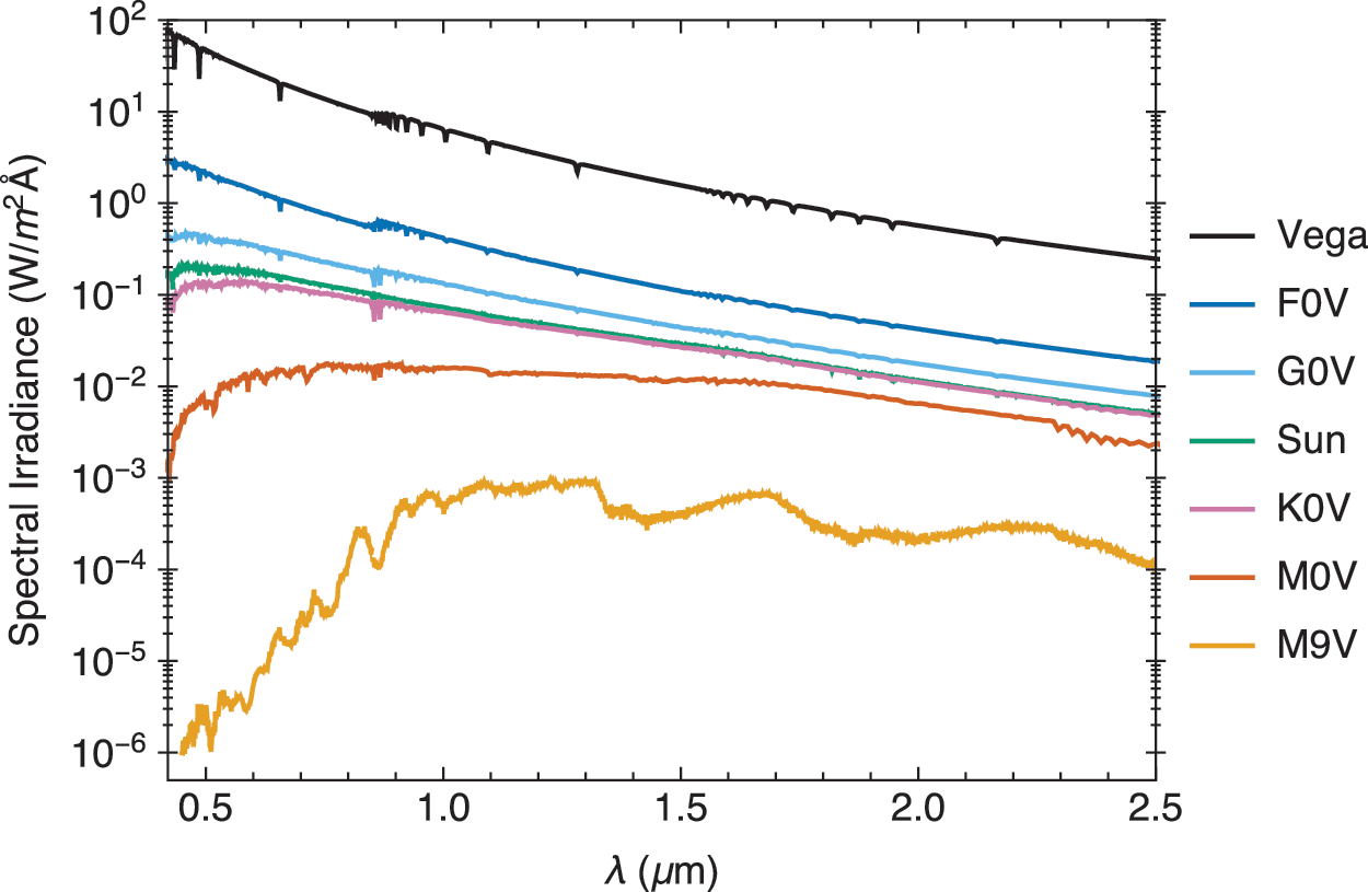
Reference spectra used for calibration (Sun and Vega) and model spectra used for host stars at 1 AU (F0V, G0V, K0V, M0V, M9V). Vega was multiplied by 1013 to fit on the same plot.

FIG. 5.

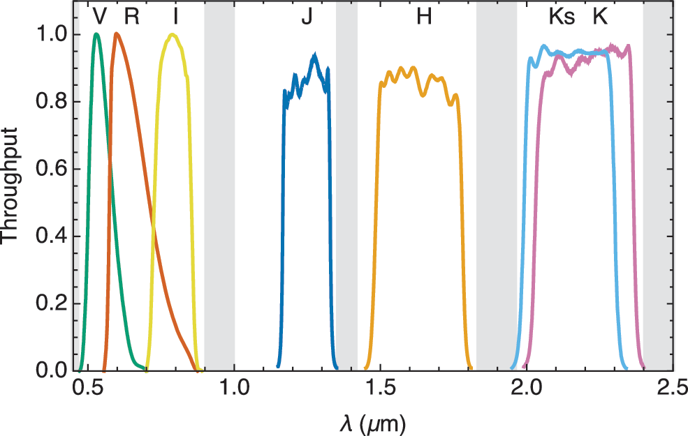
Standard filters used for flux calibration and color calculations. Gray bands show the wavelength range where the observed fluxes from the THN-PSL are not reliable.

We used this method to calibrate the THN-PSL data for each object. When comparing the coefficient of variation (CV) of the conversion factors for each body, we found that the data showed two distinct groups, one with a CV >14% and another with a CV <6%. We use that distinction to set the level of the conversion factor for uncontaminated spectra to (CV >6%) over the different filter bins. If the CV value was in the second group (CV >14%), the data are flagged as contaminated and not used in our catalog. The nature of this contamination is unclear, it could be photometric error during the observation, excess light from the host planet, or other effects that influenced the observations. The values calculated for k_V , \documentclass{aastex}\usepackage{amsbsy}\usepackage{amsfonts}\usepackage{amssymb}\usepackage{bm}\usepackage{mathrsfs}\usepackage{pifont}\usepackage{stmaryrd}\usepackage{textcomp}\usepackage{portland, xspace}\usepackage{amsmath, amsxtra}\usepackage{upgreek}\pagestyle{empty}\DeclareMathSizes{10}{9}{7}{6}\begin{document}$$\;{k_R}$$ \end{document} , \documentclass{aastex}\usepackage{amsbsy}\usepackage{amsfonts}\usepackage{amssymb}\usepackage{bm}\usepackage{mathrsfs}\usepackage{pifont}\usepackage{stmaryrd}\usepackage{textcomp}\usepackage{portland, xspace}\usepackage{amsmath, amsxtra}\usepackage{upgreek}\pagestyle{empty}\DeclareMathSizes{10}{9}{7}{6}\begin{document}$$\;{k_I}$$ \end{document} , \documentclass{aastex}\usepackage{amsbsy}\usepackage{amsfonts}\usepackage{amssymb}\usepackage{bm}\usepackage{mathrsfs}\usepackage{pifont}\usepackage{stmaryrd}\usepackage{textcomp}\usepackage{portland, xspace}\usepackage{amsmath, amsxtra}\usepackage{upgreek}\pagestyle{empty}\DeclareMathSizes{10}{9}{7}{6}\begin{document}$$\;{k_J}$$ \end{document} , and \documentclass{aastex}\usepackage{amsbsy}\usepackage{amsfonts}\usepackage{amssymb}\usepackage{bm}\usepackage{mathrsfs}\usepackage{pifont}\usepackage{stmaryrd}\usepackage{textcomp}\usepackage{portland, xspace}\usepackage{amsmath, amsxtra}\usepackage{upgreek}\pagestyle{empty}\DeclareMathSizes{10}{9}{7}{6}\begin{document}$$\;k$$ \end{document} , and the CV for each observation are given in Appendix Table A1.

2.2. Albedos of solar system bodies

We then derive the geometric albedo from the calibrated spectra as a second part of our analysis (see Tables 1 and 2 for references) by dividing the observed flux of the solar system bodies by the solar flux and accounting for the observation geometry as given in Equation 5 (de Vaucouleurs, 1964). \documentclass{aastex}\usepackage{amsbsy}\usepackage{amsfonts}\usepackage{amssymb}\usepackage{bm}\usepackage{mathrsfs}\usepackage{pifont}\usepackage{stmaryrd}\usepackage{textcomp}\usepackage{portland, xspace}\usepackage{amsmath, amsxtra}\usepackage{upgreek}\pagestyle{empty}\DeclareMathSizes{10}{9}{7}{6}\begin{document} \begin{align*} p = { \frac { { d^2 } a_b^2f } { \phi \left( \alpha \right) R_b^2a_ \oplus ^2 { f_ { sun } } } } , \tag { 5 } \end{align*} \end{document}

Table 1.

Parameters for the 10 Solar System Bodies from the THN-PSL We Used to Calculate the Calibrated Flux and Albedos

Name	Observation date	V mag.	d (AU)	a_b (AU)	R_b (km)	α (deg.)	φ (α)	Phase reference	Albedo ref.
Ceres	11/25/08	8.40	2.405	2.558	470	23	0.34(5)	Reddy et al. (2015)	Reddy et al. (2015)
Dione	5/5/08	10.40	8.97	9.298	560	6	0.88(3)	Buratti and Veverka (1984)	Noll et al. (1997), Cassini VIMS—NASA PDS
Earth	11/21/08	−2.50	0.0026^a	0.988^a	6378	70	0.5	Goode et al. (2001)	Kaltenegger et al. (2010), Meadows (2006)
Jupiter	5/7/08	−2.40	4.68	5.199	71,492	10	0.91(8)	Irvine et al. (1968)	Karkoschka (1998)
Moon	11/21/08	−9.30	0.00261	0.988	1738	108	0.05(1)	Lane and Irvine (1973)	Lane and Irvine (1973)
Neptune 1	5/7/08	7.90	30.14	30.04	24,766	2	1	Pollack et al. (1986)	Karkoschka (1998), Fink and Larson (1979)
Neptune 2	11/20/08	7.90	30.145	30.03	24,766	2	1	Pollack et al. (1986)	Karkoschka, 1998, Fink and Larson (1979)
Neptune 3	11/25/08	7.90	30.23	30.03	24,766	2	1	Pollack et al. (1986)	Karkoschka, 1998, Fink and Larson (1979)
Neptune 4	11/26/08	7.90	30.247	30.03	24,766	2	1	Pollack et al. (1986)	Karkoschka, 1998, Fink and Larson, 1979)
Pluto^b	5/11/08	15.00	30.72	31.455	1150	1	1		Lorenzi et al. (2016); Protopapa et al. (2008)
Rhea	11/25/08	9.90	9.591	9.36	764	6	0.87(2)	Buratti and Veverka (1984)	Noll et al. (1997), Cassini VIMS—NASA PDS
Saturn 1	5/5/08	1.00	8.97	9.296	60,268	6	0.76(3)	Irvine et al. (1968)	Karkoschka (1998), Fink and Larson (1979)
Saturn 2	11/19/08	1.20	9.685	9.356	60,268	6	1	Irvine et al. (1968)	Karkoschka (1998), Fink and Larson (1979)
Saturn 3	11/19/08	1.20	9.685	9.356	60,268	6	0.76(3)	Irvine et al. (1968)	Karkoschka (1998), Fink and Larson (1979)
Saturn 4	11/22/08	1.20	9.6385	9.359	60,268	6	0.76(3)	Irvine et al. (1968)	Karkoschka (1998), Fink and Larson (1979)
Titan 1	5/5/08	8.40	8.97	9.3	2575	6	0.98(3)	Tomasko and Smith (1982)	Karkoschka (1998), Fink and Larson (1979)
Titan 2	5/6/08	8.40	8.97	9.3	2575	6	0.98(3)	Tomasko and Smith (1982)	Karkoschka (1998), Fink and Larson (1979)
Titan 3	11/24/08	8.60	9.5947	9.364	2575	6	0.98(3)	Tomasko and Smith (1982)	Karkoschka (1998), Fink and Larson (1979)
Uranus 1	5/11/08	5.90	20.66	20.097	25,559	2	1	Pollack et al. (1986)	Karkoschka (1998), Fink and Larson (1979)
Uranus 2	11/20/08	5.80	19.742	20.097	25,559	3	1	Pollack et al. (1986)	Karkoschka (1998), Fink and Larson (1979)

References used for phase function and albedo.

To obtain the proper geometric albedo for this Earthshine observation, a factor of 2.38E5 is needed.

The Pluto–Charon spectrum is added for completeness.

THN-PSL = Tohoku-Hiroshima-Nagoya Planetary Spectral Library.

Table 2.

Data for the Solar System Bodies from the THN-PSL Data Set That Were Contaminated Based on the Shape of Their Calculated Geometric Albedo

Name	Observation date	V Mag.	d (AU)	a_b (AU)	R_b (km)	α (deg.)	φ (α)		Albedo Ref.
Callisto^a	5/5/08	6.30	4.73	5.214	2410	10	0.60(2)	Squyres and Veverka (1981)	Spencer (1987), Spencer et al. (1995)
Europa	5/7/08	5.60	4.69	5.195	1565	10	0.88(5)	Buratti and Veverka (1983), Buratti and Veverka (1984)	Buratti and Veverka (1983), Spencer (1987), Spencer et al. (1995)
Ganymede	11/26/08	5.40	5.7518	5.12066	2634	8	0.80(5)	Squyres and Veverka (1981)	Spencer (1987), Spencer et al. (1995)
Io	11/26/08	5.80	5.7556	5.12348	1821	8	0.87(5)	Simonelli and Veverka (1984)	Spencer et al. (1995), Fanale et al. (1974)
Mars	5/12/08	1.30	1.68	1.6676	3397	35	0.58(5)	Irvine et al. (1968)	McCord and Westphal (1971), Meadows (2006)
Mercury	5/11/08	0.00	0.99	0.37547	2440	96	0.11(5)	Irvine et al. (1968), Mallama et al. (2002)	Mallama et al. (2002), Mallama (2017)
Venus	11/20/08	−4.20	1.077	0.72556	6052	63	0.4(1)	Irvine et al. (1968)	Meadows (2006), Kaltenegger et al. (2010)

Note that the authors state that the Callisto data are contaminated.

where d is the separation between Earth and the body, a_b the distance between the Sun and the body at the time of observation, and \documentclass{aastex}\usepackage{amsbsy}\usepackage{amsfonts}\usepackage{amssymb}\usepackage{bm}\usepackage{mathrsfs}\usepackage{pifont}\usepackage{stmaryrd}\usepackage{textcomp}\usepackage{portland, xspace}\usepackage{amsmath, amsxtra}\usepackage{upgreek}\pagestyle{empty}\DeclareMathSizes{10}{9}{7}{6}\begin{document}$${a_ \oplus}$$ \end{document} the semimajor axis of Earth. \documentclass{aastex}\usepackage{amsbsy}\usepackage{amsfonts}\usepackage{amssymb}\usepackage{bm}\usepackage{mathrsfs}\usepackage{pifont}\usepackage{stmaryrd}\usepackage{textcomp}\usepackage{portland, xspace}\usepackage{amsmath, amsxtra}\usepackage{upgreek}\pagestyle{empty}\DeclareMathSizes{10}{9}{7}{6}\begin{document}$${f_{sun}}$$ \end{document} and f are the fluxes from the Sun seen from Earth and the body seen from Earth, respectively, R_b is the radius of the body being observed, and \documentclass{aastex}\usepackage{amsbsy}\usepackage{amsfonts}\usepackage{amssymb}\usepackage{bm}\usepackage{mathrsfs}\usepackage{pifont}\usepackage{stmaryrd}\usepackage{textcomp}\usepackage{portland, xspace}\usepackage{amsmath, amsxtra}\usepackage{upgreek}\pagestyle{empty}\DeclareMathSizes{10}{9}{7}{6}\begin{document}$$\phi \left( \alpha \right)$$ \end{document} is the value of the phase function at the point in time the observation was taken. For \documentclass{aastex}\usepackage{amsbsy}\usepackage{amsfonts}\usepackage{amssymb}\usepackage{bm}\usepackage{mathrsfs}\usepackage{pifont}\usepackage{stmaryrd}\usepackage{textcomp}\usepackage{portland, xspace}\usepackage{amsmath, amsxtra}\usepackage{upgreek}\pagestyle{empty}\DeclareMathSizes{10}{9}{7}{6}\begin{document}$${f_{sun}}$$ \end{document} , we used the standard Space Telescope Imaging Spectrograph Sun spectrum (Bohlin et al., 2001)³ shown in Fig. 4. If the geometric albedo exceeds 1, the data are flagged as contaminated and not used in our catalog.

Note that we also compared the spectra that were flagged as contaminated in this two-step analysis with the available data and models from other groups (Fig. 3). All flagged spectra show a strong difference in albedo for these bodies observed by other teams, supporting our analysis method (Fig. 3).

2.3. Using colors to characterize planets

We use a standard astronomy tool, a color–color diagram, to analyze whether we can distinguish solar system bodies based on their colors and what effect resolution and filter choice has on this analysis. Several teams have shown that photometric colors of planetary bodies can be used to initially distinguish between icy, rocky, and gaseous surface types (Traub, 2003; Lundock et al., 2009; Cahoy et al., 2010; Krissansen-Totton et al., 2016). We calculated the colors from high- and low-resolution spectra to mimic early results from exoplanet observations as well as explored the effect of spectral resolution on the colors and their interpretation. The error for colors derived from the THN-PSL data was calculated by adding the errors used by Lundock et al. (2009) and the error accumulated through the conversion process of 6% in the k value. This gives \documentclass{aastex}\usepackage{amsbsy}\usepackage{amsfonts}\usepackage{amssymb}\usepackage{bm}\usepackage{mathrsfs}\usepackage{pifont}\usepackage{stmaryrd}\usepackage{textcomp}\usepackage{portland, xspace}\usepackage{amsmath, amsxtra}\usepackage{upgreek}\pagestyle{empty}\DeclareMathSizes{10}{9}{7}{6}\begin{document}$$\Delta \left( {J - K} \right) = \pm 0.34$$ \end{document} and \documentclass{aastex}\usepackage{amsbsy}\usepackage{amsfonts}\usepackage{amssymb}\usepackage{bm}\usepackage{mathrsfs}\usepackage{pifont}\usepackage{stmaryrd}\usepackage{textcomp}\usepackage{portland, xspace}\usepackage{amsmath, amsxtra}\usepackage{upgreek}\pagestyle{empty}\DeclareMathSizes{10}{9}{7}{6}\begin{document}$$\Delta \left( {R - J} \right) = \pm 0.28$$ \end{document} for the error values. We reduce the high-resolution data of \documentclass{aastex}\usepackage{amsbsy}\usepackage{amsfonts}\usepackage{amssymb}\usepackage{bm}\usepackage{mathrsfs}\usepackage{pifont}\usepackage{stmaryrd}\usepackage{textcomp}\usepackage{portland, xspace}\usepackage{amsmath, amsxtra}\usepackage{upgreek}\pagestyle{empty}\DeclareMathSizes{10}{9}{7}{6}\begin{document}$$R = 138 - 360$$ \end{document} to \documentclass{aastex}\usepackage{amsbsy}\usepackage{amsfonts}\usepackage{amssymb}\usepackage{bm}\usepackage{mathrsfs}\usepackage{pifont}\usepackage{stmaryrd}\usepackage{textcomp}\usepackage{portland, xspace}\usepackage{amsmath, amsxtra}\usepackage{upgreek}\pagestyle{empty}\DeclareMathSizes{10}{9}{7}{6}\begin{document}$$R = 8$$ \end{document} to mimic colors that are generated from low-resolution spectra as shown in Fig. 6. The colors at high resolutions were used to determine the best color–color combination for surface and atmospheric characterization, a process that was repeated for colors derived from low-resolution spectra.

FIG. 6.

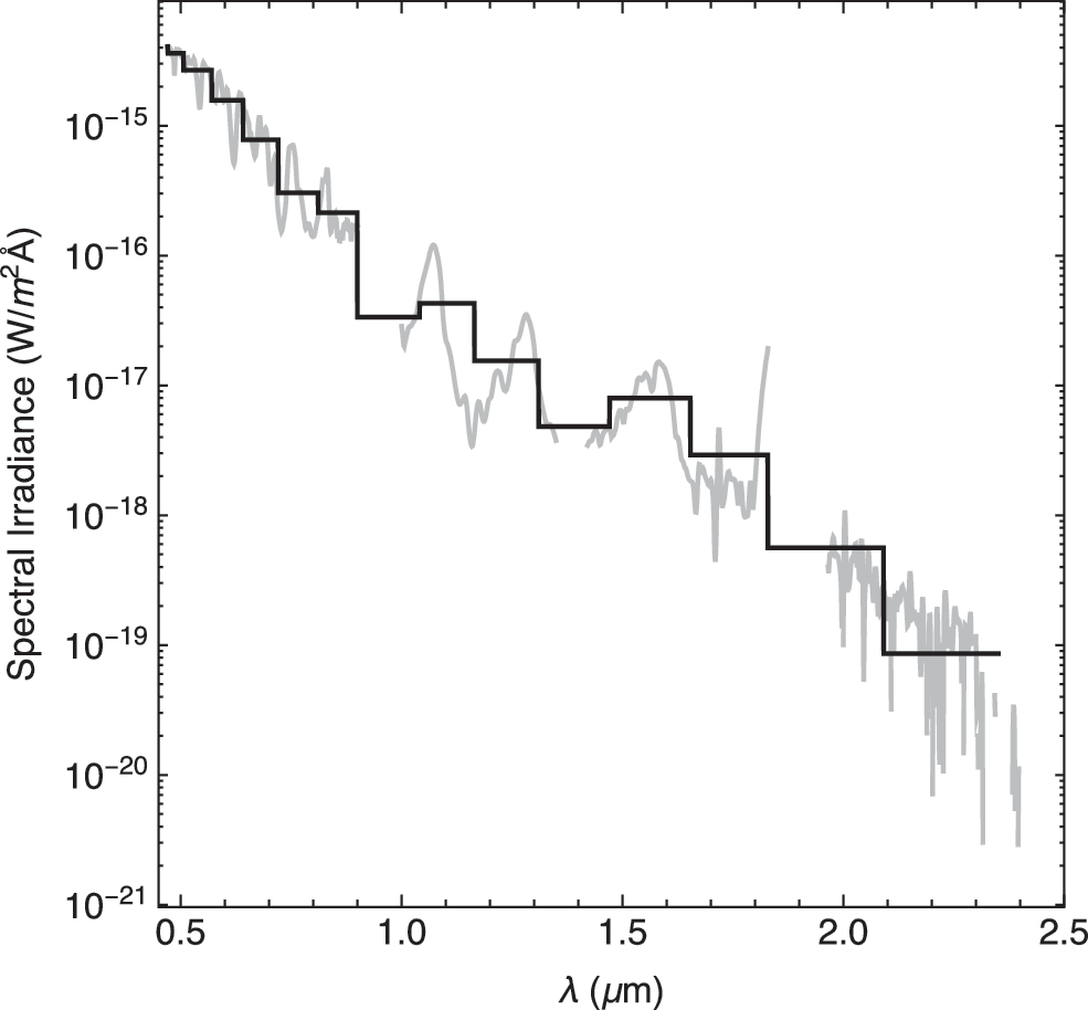
An example of a reduced resolution spectrum compared with its high-resolution observations.

We also explored how to characterize solar system analog planets around other host stars using their colors by placing the bodies at an equivalent orbital distance around different host stars (F0V, G0V, K0V, M0V, and M9V). We used stellar spectra for the host stars from the Castelli and Kurucz Atlas (Castelli and Kurucz, 2004)⁴ and the PHOENIX library (Husser et al., 2013)⁵ (Fig. 4). As a first-order approximation, we have assumed that the albedo of the object would not change under this new incoming stellar flux (Section 4).

3. Results

3.1. A spectra and albedo catalog of a diverse set of solar system objects

We assembled a reference catalog of 19 bodies in our solar system as a baseline for comparison with upcoming exoplanet observations. To provide a wide range of solar system bodies in our catalog, we compiled and analyzed data from uncalibrated and calibrated spectra of previously published disk-integrated observations. Our catalog contains spectra and geometric albedo of the eight planets: Mercury (Mallama, 2017), Venus (Pollack et al., 1978; Meadows, 2006), Earth (Lundock et al., 2009), Mars (McCord and Westphal, 1971), Jupiter, Saturn, Uranus, and Neptune (Lundock et al., 2009). Nine moons: Io (Fanale et al., 1974), Callisto, Europa, Ganymede (Spencer, 1987), Enceladus⁶ (Filacchione et al., 2012), Dione, Rhea, the Moon, and Titan (Lundock et al., 2009), and two dwarf planets: Ceres (Lundock et al., 2009) and Pluto (Protopapa et al., 2008; Lorenzi et al., 2016).

For the eight planets of the Solar System, nine moons (Callisto, Dione, Europa, Ganymede, Io, the Moon, Rhea, and Titan), and two dwarf planets (Ceres and Pluto), we present the absolute fluxes in Fig. 1 and the geometric albedos in Fig. 2.

3.2. Contaminated spectra in the THN-PSL data set

When we derived the geometric albedo from the calibrated THN-PSL spectra as the second part of our analysis, we found that six objects (Io, Europa, Ganymede, Mercury, Mars, and Venus) display geometric albedos exceeding 1, indicating that the measurements are contaminated (Table 2 and Fig. 3). We compared the albedo of these six observations with previously published values in the literature (McCord and Westphal, 1971; Fanale et al., 1974; Pollack et al., 1978; Buratti and Veverka, 1983; Spencer, 1987; Spencer et al., 1995; Mallama et al., 2002; Meadows, 2006; Mallama, 2017) and found substantial differences over the wavelength covered by the different teams (Fig. 3). We list the seven bodies with contaminated THN-PSL measurements in Table 2.

3.3. Spectra not flagged as contaminated in the THN-PSL data set

Table 1 lists the spectra of the 10 bodies from the THN-PSL database, which were not flagged as contaminated and are part of our catalog, as well as the Pluto–Charon spectrum. It shows the properties we used to calculate their albedos, once we un-normalized the uncalibrated data as well as references to previously published albedos. Note that we did not use the THN-PSL Pluto–Charon spectrum in our analysis because it is not a Pluto spectrum. Instead we use the spectrum for Pluto published by two teams (Protopapa et al., 2008; Lorenzi et al., 2016) that cover the wavelength range required for our analysis. We show both spectra in Fig. 3 for completeness.

We compared the derived albedo of the 10 bodies from the THN-PSL database, which were not flagged as contaminated, against disk-integrated spectra and albedo from observations or models in the literature for the wavelengths available. Our derived albedos are in qualitative agreement with previously published data (Fig. 3) for Ceres (Reddy et al., 2015); Dione and Rhea (Cassini VIMS; Noll et al., 1997); Earth (Meadows, 2006; Kaltenegger et al., 2010); the Moon (Lane and Irvine, 1973); and Jupiter, Saturn, Uranus, Neptune, and Titan (Fink and Larson, 1979; Karkoschka, 1998). We simulated their absolute fluxes with the same observation geometry as the THN-PSL spectra to be able to compare them (Fig. 3). Note that small changes are likely due to observation geometry as well as the changes in the atmospheres over the time between observations. Gaseous bodies are known to have daily variations in brightness (Belton et al., 1981). For completeness, we include the THN-PSL observation of the combined spectrum of Pluto and Charon and compare it with the albedo of Pluto (Protopapa et al., 2008; Lorenzi et al., 2016). We averaged several Cassini VIMS observations together and used them as references for Rhea and Dione.⁷

3.4. Using color–color diagrams to initially characterize solar system bodies

To qualify the solar system objects in terms of extrasolar planet observables, we consider whether they are gaseous, icy, or rocky bodies and do not distinguish between moons and planets. Thus, Titan and Venus are both gaseous bodies in our analysis since only their atmosphere is being observed at this wavelength range.

Figure 7 shows the spectra as well as the colors for the three subcategories in our catalog. The top panel shows gaseous bodies: Jupiter, Saturn, Uranus, Neptune, Venus, and Titan. The middle panel shows rocky bodies: Mars, Mercury, Io, Ceres, Earth, and the Moon. The bottom panel shows icy bodies: Ganymede, Dione, Rhea, Callisto, Pluto, Europa, and Enceladus. Each surface type occupies its own color space in the diagram.

FIG. 7.

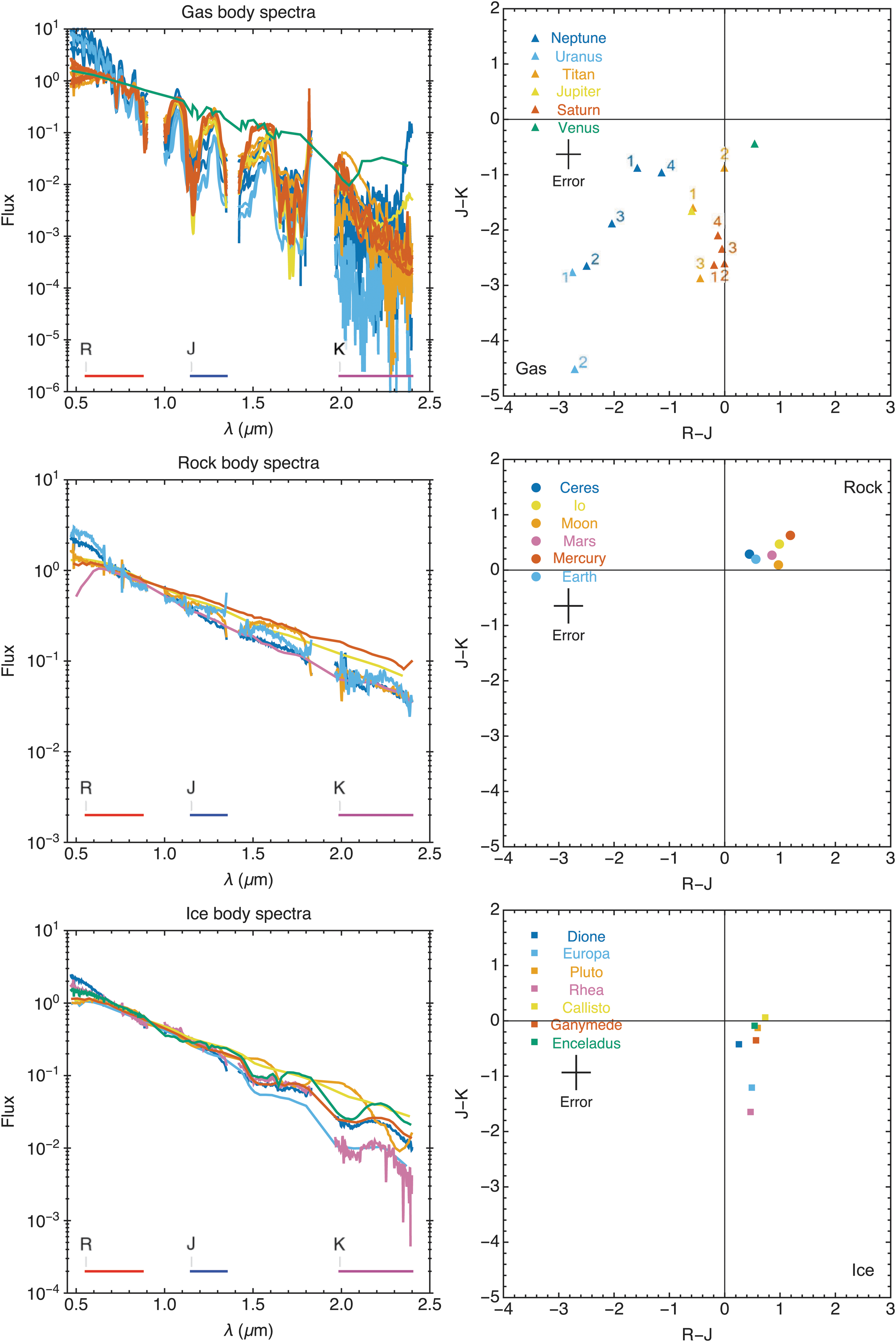
Spectra and color–color diagrams for gaseous, rocky, and icy bodies of the Solar System. Previously published data were used for bodies that were contaminated in the THN-PSL following the references in Fig. A1.

To explore how the resolution of the available spectra and thus the observation time available would influence this classification, we reduced the spectral resolution for all spectra to \documentclass{aastex}\usepackage{amsbsy}\usepackage{amsfonts}\usepackage{amssymb}\usepackage{bm}\usepackage{mathrsfs}\usepackage{pifont}\usepackage{stmaryrd}\usepackage{textcomp}\usepackage{portland, xspace}\usepackage{amsmath, amsxtra}\usepackage{upgreek}\pagestyle{empty}\DeclareMathSizes{10}{9}{7}{6}\begin{document}$$R = \lambda / \Delta \lambda$$ \end{document} of 8. We find that the derived colors of the solar system bodies do not shift substantially (Fig. 8), showing that colors derived from high- and low-resolution spectra provide similar capabilities for first-order color characterization of a solar system object. Although a slight shift occurs in the color–color diagram, the three different solar system surface types (gaseous, rocky, and icy) can still be distinguished, showing that colors from low-resolution spectra can be used for first-order characterization of bodies in our solar system. We chose a lower resolution of \documentclass{aastex}\usepackage{amsbsy}\usepackage{amsfonts}\usepackage{amssymb}\usepackage{bm}\usepackage{mathrsfs}\usepackage{pifont}\usepackage{stmaryrd}\usepackage{textcomp}\usepackage{portland, xspace}\usepackage{amsmath, amsxtra}\usepackage{upgreek}\pagestyle{empty}\DeclareMathSizes{10}{9}{7}{6}\begin{document}$$R = 8$$ \end{document} since the bin width near the K-band becomes larger than the K-band filter itself at lower resolutions. Bandwidth is directly proportional to the amount of light collected by a telescope and thus the time needed for observation. If low-resolution spectra could initially characterize a planet, exoplanets could be prioritized for time-intense high-resolution follow-up observations from their colors. At a lower resolution, a higher signal-to-noise ratio is required to achieve the same distinguishability as an observation at high resolution. The ratio of the integral uncertainties of two spectra at different resolutions, \documentclass{aastex}\usepackage{amsbsy}\usepackage{amsfonts}\usepackage{amssymb}\usepackage{bm}\usepackage{mathrsfs}\usepackage{pifont}\usepackage{stmaryrd}\usepackage{textcomp}\usepackage{portland, xspace}\usepackage{amsmath, amsxtra}\usepackage{upgreek}\pagestyle{empty}\DeclareMathSizes{10}{9}{7}{6}\begin{document}$${ \rm{ \Delta }}{I_A}$$ \end{document} and \documentclass{aastex}\usepackage{amsbsy}\usepackage{amsfonts}\usepackage{amssymb}\usepackage{bm}\usepackage{mathrsfs}\usepackage{pifont}\usepackage{stmaryrd}\usepackage{textcomp}\usepackage{portland, xspace}\usepackage{amsmath, amsxtra}\usepackage{upgreek}\pagestyle{empty}\DeclareMathSizes{10}{9}{7}{6}\begin{document}$${ \rm{ \Delta }}{I_B}$$ \end{document} , is proportional to the number of bins being integrated over, N, and the measurement uncertainty of each bin, \documentclass{aastex}\usepackage{amsbsy}\usepackage{amsfonts}\usepackage{amssymb}\usepackage{bm}\usepackage{mathrsfs}\usepackage{pifont}\usepackage{stmaryrd}\usepackage{textcomp}\usepackage{portland, xspace}\usepackage{amsmath, amsxtra}\usepackage{upgreek}\pagestyle{empty}\DeclareMathSizes{10}{9}{7}{6}\begin{document}$$\delta m$$ \end{document} , as shown in Equation 6. \documentclass{aastex}\usepackage{amsbsy}\usepackage{amsfonts}\usepackage{amssymb}\usepackage{bm}\usepackage{mathrsfs}\usepackage{pifont}\usepackage{stmaryrd}\usepackage{textcomp}\usepackage{portland, xspace}\usepackage{amsmath, amsxtra}\usepackage{upgreek}\pagestyle{empty}\DeclareMathSizes{10}{9}{7}{6}\begin{document} \begin{align*}{ \frac { { \rm { \Delta } } { I_A } } { { \rm { \Delta } } { I_B } } } \propto \sqrt { { \frac { { N_B } } { { N_A } } } } { \frac { \delta { m_A } } { \delta { m_B } } } \tag { 6 } \end{align*} \end{document}

FIG. 8.

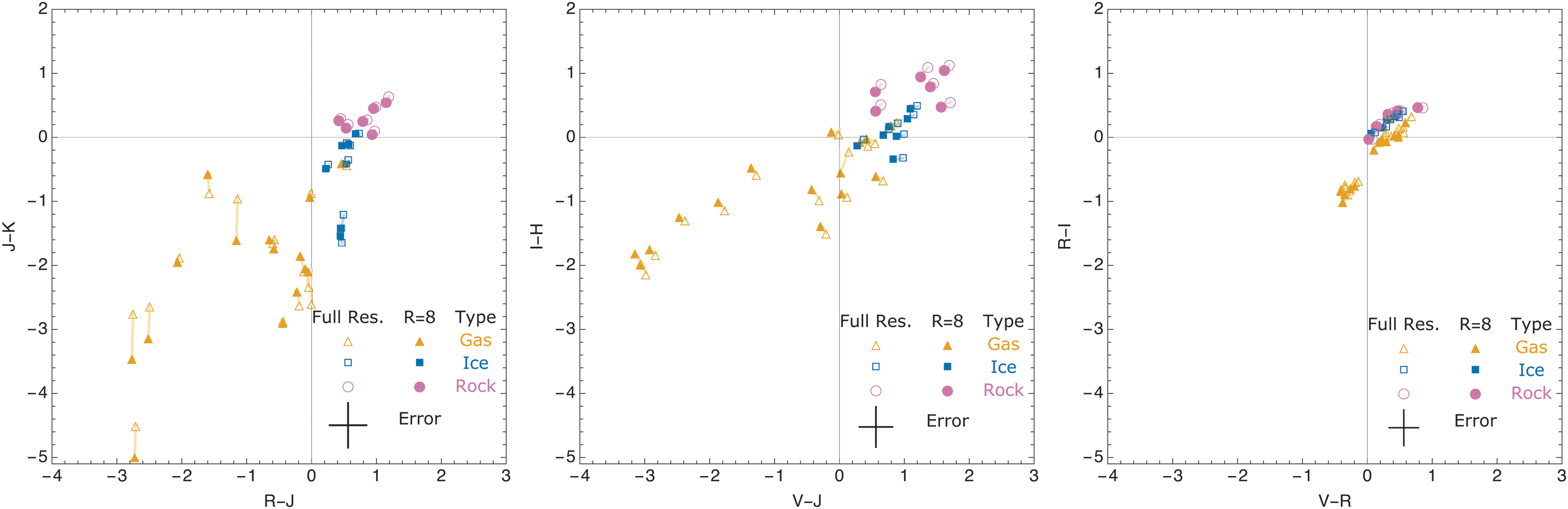
Comparison of colors calculated using low- (filled symbols, \documentclass{aastex}\usepackage{amsbsy}\usepackage{amsfonts}\usepackage{amssymb}\usepackage{bm}\usepackage{mathrsfs}\usepackage{pifont}\usepackage{stmaryrd}\usepackage{textcomp}\usepackage{portland, xspace}\usepackage{amsmath, amsxtra}\usepackage{upgreek}\pagestyle{empty}\DeclareMathSizes{10}{9}{7}{6}\begin{document}$$R = 8$$ \end{document} ) versus high-resolution (nonfilled symbols, R = 138, 142, and 360 for THN-PSL data) spectra for 19 solar system bodies around the Sun. Each panel shows a different filter combination and the symbols represent the three surface types: gaseous (square), icy (triangle), and rocky (circle).

We explored different filter combinations to best distinguish between icy, gaseous, and rocky bodies. We find that R-J versus J-K colors distinguish the bodies best (see also Traub, 2003; Lundock et al., 2009; Cahoy et al., 2010; Krissansen-Totton et al., 2016).

If only a smaller wavelength range is available, such as V through H or V through I, Fig. 8 shows which alternative filter combinations can still separate the surface types. However, Fig. 8 shows that a wider wavelength range improves the characterization of surfaces for solar system objects substantially. The success of using this method to characterize the Solar System reduces with narrower wavelength coverage. Long wavelengths (J and K band) especially help distinguish different kinds of Solar System bodies (Fig. 8). To characterize all bodies in the solar system, it is important to have wavelength coverage of the visible and near IR at a resolution that distinguishes each band.

3.5. Colors of solar system analog bodies orbiting different host stars

To provide observers with the color space where solar system analog exoplanets could be found, we use the albedos shown in Fig. 2 to explore the colors of similar bodies orbiting different host stars. For airless bodies, the albedo is a direct surface measurement; therefore, that assumption should be valid for similar surface composition. For objects with substantial atmospheres that can be influenced by stellar radiation, individual models are needed to assess whether the albedo of a system's bodies would notably change due to the different host star flux. Note that Earth's albedo would not change significantly from F0V to M9V host stars in the wavelength range considered here (see Rugheimer et al., 2013, 2015).

Figure 9 shows the colors of the solar system analog bodies orbiting other host stars. Because their albedo is assumed to be constant, the shift closely mimics the shift in colors of the host star. For hotter host stars, the colors shift to a bluer section of the color–color diagram (F0V). For cooler host stars, the colors shift toward a redder portion of the color space (M0V and M9V). This provides insights for observers into where the divisions in color space of rocky, icy, and gaseous bodies lie depending on the host star's spectral class.

FIG. 9.

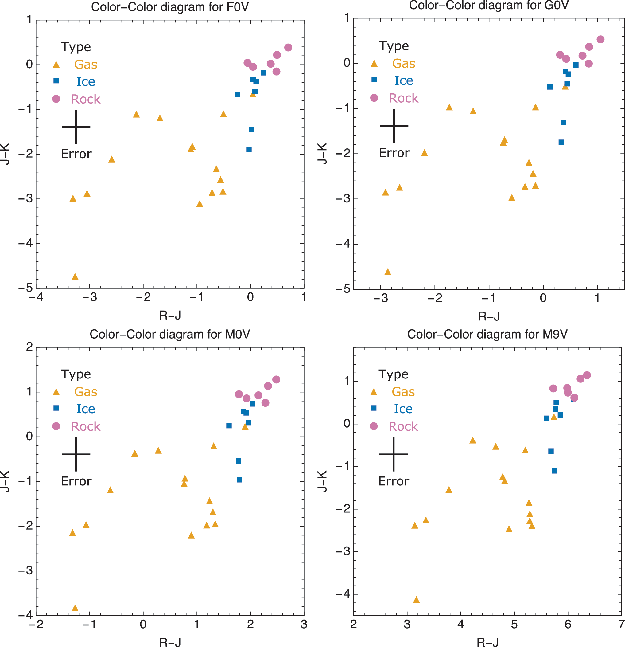
Colors of solar system bodies around different host stars. Here we show the colors of solar system bodies for an F0V (upper left), a G0V (upper right), an M0V (lower left), and an M9V (lower right) host star.

4. Discussion

4.1. Change in colors of gaseous planets

Some gaseous bodies in the THN-PSL with multiple spectra (Uranus, Neptune, and Titan) show variations in their colors larger than the error (Fig. 7). Gaseous bodies are known to vary in brightness over timescales shorter than the time between these observations (Belton et al., 1981), consistent with the THN-PSL data. This indicates that any subdivide for gaseous bodies would be challenging from their colors alone. However, the K-band is also more susceptible to photometric error as discussed in the THN-PSL article (Lundock et al., 2009), which could add to the observed differences. Multiple uncontaminated observations across the same wavelengths for rocky or icy bodies are not available in the literature; therefore, we cannot assess whether a spread in colors also exists for rocky or icy bodies, independent of viewing geometry.

4.2. Nondisk-integrated spectra of some objects

Owing to the finite field of view of the TRISPEC instrument, the observations of Earth, Moon, Jupiter, and Saturn were not disk integrated. A disk-integrated spectrum is preferred because it averages the light from the entire body instead of from a small region of its surface. The spectrograph slit was centered on the planet and aligned longitudinally for Jupiter and Saturn, making the spectra as representative of the entire surface as possible. When comparing their spectra with other sources, the spectra show a good match to disk-integrated spectra (Fink and Larson, 1979; Karkoschka, 1998). This could not be done for the Moon and the Earthshine observations, leading to variations in their spectra from previously published data.

4.3. Spectra derived from the THN-PSL data set

We have used several spectra of planets and moons from the THN-PSL data set that did not appear contaminated in our analysis. The contamination of six objects in the THN-PSL database raises questions about the viability of the spectra in this database in general. We compared the 10 bodies that we used in our catalog, which were not flagged as contaminated against disk-integrated spectra and albedo from observations or models in the literature. These observations or models were not available for the whole wavelength range, thus we could not compare the full wavelength range; however, the range covered shows qualitative agreement with previously published data (Fig. 3) and thus we have included the spectra and albedos we derived from the uncalibrated THN-PSL data in our analysis. For Earth and the Moon, time variability of the spectra can be explained because observations of Earth and the Moon were not disk integrated, due to the spectrographic slit as discussed in Section 4.2. Note that for most solar system objects, reliable disk-averaged spectra for different times are lacking, which are observations that would be useful for future exoplanet comparisons.

4.4. Similarity of the color of water and rock

The primarily liquid water surface of Earth is unique in the Solar System; however, this is not apparent in the color–color diagrams (Figs. 7 –9). This is because water and rock share a similar relatively flat albedo over the 0.5–2.5 μm wavelength range. This specific color–color degeneracy for rock and water can be broken if shorter wavelength observations are available (see also Krissansen-Totton et al., 2016).

4.5. Color of CO₂ atmospheres appears similar to icy surfaces

Venus has the interesting position of being a rocky planet that has a gaseous appearance but lies among the colors of the icy bodies in the color–color diagrams. This is due to Venus having a primarily CO₂ atmosphere, which provides a similarly sloped albedo as ice in this wavelength range. This shows the limits of initial characterization through a color–color diagram. It will make habitability assessments from colors alone of terrestrial planets especially on the edges of their habitable zones very difficult since CO₂ is likely to be present. Estimates of the effective stellar flux that reaches the planet or moon could help to disentangle the ice/CO₂ degeneracy on the inner edge of the habitable zone. On the outer edge of the habitable zone, both surface types should be present, CO₂-rich atmospheres and icy bodies; therefore, higher resolution spectra will be needed to break such degeneracy.

4.6. Spotting the absence of methane in a gas planet's colors

The absence of methane in Venus' atmosphere makes it distinguishable from the other gaseous objects in our solar system in the color–color diagrams. More information about the atmospheric composition of exoplanets and exomoons would be needed before we can assess whether we could derive similar inferences for other planetary systems.

4.7. Colors of objects that are made of “dirty snow”

In the color–color diagrams, Ganymede and Callisto fall in the region between rocky and ice bodies due to their high amount of “dirty snow” compared with the other bodies in the icy body category. Given the error bars in their colors, these two bodies could be placed in either the rocky or icy categories. Such rocky–icy bodies are anticipated in other planetary systems as well and should lie in the color space between the icy and rocky bodies like in our solar system.

5. Conclusions

We present a catalog of spectra and geometric albedos for 19 solar system bodies, which are representative of the types of surfaces found throughout the Solar System for wavelengths from 0.45 to 2.5 μm. This catalog provides a baseline for comparison of exoplanet observations with the most closely studied bodies in our solar system. The data used and created in this article are available for download through the Carl Sagan Institute.⁸

We show the utility of a color–color diagram to distinguish between rocky, icy, and gaseous bodies in our solar system for colors derived from high- as well as low-resolution spectra (Figs. 7 and 8) and initially characterize extrasolar planets and moons. The spectra, albedo, and colors presented in this catalog can be used to prioritize time-intensive follow-up spectral observations of extrasolar planets and moons with current and next generation like the extremely large telescopes. Assuming an unchanged albedo, solar system body analog exoplanets shift their position in a color–color diagram following the color change of the host stars (Fig. 9). Detailed spectroscopic characterization will be necessary to confirm the provisional categorization from the broadband photometry suggested here, which is only based on planets and moons of our own solar system.

Planetary science broke new ground in the 70s and 80s with spectral measurements for solar system bodies. Exoplanet science will see a similar renaissance in the near future, when we will be able to compare spectra of a wide range of exoplanets with the catalog of bodies in our solar system.

Footnotes

Acknowledgments

Thanks to Gianrico Filacchione, Ramsey Lundock, Erich Karkoschka, Siddharth Hegde, Paul Helfenstein, Steve Squyres, and our reviewers for helpful discussions and comments. The authors acknowledge support by the Simons Foundation (SCOL No. 290357, Kaltenegger), the Carl Sagan Institute, and the NASA/New York Space Grant Consortium (NASA Grant No. NNX15AK07H).

Author Disclosure Statement

No competing financial interests exist.

Abbreviations Used

Appendix Table A1.

Calculated k Values for Each Band and Their Average for Each Observation

Name	Observation date	k_V	k_R	k_I	k_J	k	Standard deviation	CV (%)
Uncontaminated (CV <6% and albedo <1)
Ceres	11/25/08	8.27E-16	8.27E-16	8.45E-16	8.36E-16	8.34E-16	8.44E-18	1.01
Dione	5/5/08	1.34E-16	1.34E-16	1.35E-16	1.34E-16	1.34E-16	6.75E-19	0.50
Earth	11/21/08	1.48E-11	1.48E-11	1.50E-11	1.50E-11	1.49E-11	1.14E-13	0.77
Jupiter	5/7/08	2.17E-11	2.16E-11	2.08E-11	2.19E-11	2.15E-11	5.03E-13	2.34
Moon	11/21/08	1.49E-08	1.49E-08	1.54E-08	1.51E-08	1.51E-08	2.27E-10	1.50
Neptune 1	5/7/08	5.28E-16	5.38E-16	4.89E-16	5.25E-16	5.20E-16	2.14E-17	4.11
Neptune 2	11/20/08	4.44E-16	4.53E-16	4.33E-16	4.42E-16	4.43E-16	8.44E-18	1.90
Neptune 3	11/25/08	2.96E-16	3.02E-16	2.86E-16	2.97E-16	2.95E-16	6.51E-18	2.20
Neptune 4	11/26/08	7.80E-16	7.94E-16	7.46E-16	7.76E-16	7.74E-16	2.00E-17	2.59
Pluto	5/11/08	2.67E-18	2.67E-18	2.70E-18	2.71E-18	2.69E-18	2.10E-20	0.78
Rhea	11/25/08	2.72E-16	2.71E-16	2.73E-16	2.73E-16	2.72E-16	1.14E-18	0.42
Saturn 1	5/5/08	8.29E-13	8.31E-13	7.86E-13	8.49E-13	8.24E-13	2.70E-14	3.28
Saturn 2	11/19/08	1.11E-12	1.10E-12	1.05E-12	1.13E-12	1.10E-12	3.44E-14	3.14
Saturn 3	11/19/08	1.00E-12	9.97E-13	9.57E-13	1.02E-12	9.94E-13	2.68E-14	2.70
Saturn 4	11/22/08	7.57E-13	7.52E-13	7.21E-13	7.62E-13	7.48E-13	1.81E-14	2.42
Titan 1	5/5/08	1.12E-15	1.13E-15	1.09E-15	1.13E-15	1.12E-15	1.79E-17	1.60
Titan 2	5/6/08	1.74E-15	1.72E-15	1.70E-15	1.76E-15	1.73E-15	2.47E-17	1.43
Titan 3	11/24/08	1.17E-15	1.16E-15	1.12E-15	1.18E-15	1.16E-15	2.45E-17	2.11
Uranus 1	5/11/08	3.04E-15	3.12E-15	2.76E-15	3.00E-15	2.98E-15	1.53E-16	5.12
Uranus 2	11/20/08	3.30E-15	3.37E-15	3.19E-15	3.26E-15	3.28E-15	7.48E-17	2.28
Contaminated (albedo >1)
Callisto	5/5/08	7.38E-15	7.36E-15	6.90E-15	7.55E-15	7.30E-15	2.78E-16	3.81
Europa	5/7/08	2.47E-14	2.46E-14	2.58E-14	2.48E-14	2.49E-14	5.57E-16	2.24
Ganymede	11/26/08	4.20E-14	4.17E-14	4.52E-14	4.26E-14	4.29E-14	1.62E-15	3.79
Io	11/26/08	1.26E-14	1.25E-14	1.41E-14	1.29E-14	1.31E-14	7.45E-16	5.70
Mars	5/12/08	1.59E-12	1.57E-12	1.73E-12	1.60E-12	1.62E-12	7.56E-14	4.67
Mercury	5/11/08	7.18E-12	7.12E-12	8.02E-12	7.31E-12	7.41E-12	4.16E-13	5.61
Venus	11/20/08	1.40E-10	1.39E-10	1.43E-10	1.39E-10	1.40E-10	2.08E-12	1.49
Contaminated (CV >14%)
Earth	5/11/08	1.84E-11	1.79E-11	1.62E-11	2.26E-11	1.88E-11	2.71E-12	14.43
Moon	11/21/08	2.08E-08	1.84E-08	2.10E-08	3.04E-08	2.26E-08	5.33E-09	23.55
Uranus	5/7/08	3.28E-15	3.22E-15	2.60E-15	7.30E-16	2.46E-15	1.19E-15	48.52

The CV and albedo (Fig. 3) were used to determine level of reliability of the observation.

CV = coefficient of variation.

References

Belton

M.J.S.

, Wallace

, and Howard

(1981) The periods of Neptune—evidence for atmospheric motions. Icarus, 46:263–274.

Bessell

M.S.

(1979) UBVRI photometry. II—the cousins VRI system, its temperature and absolute flux calibration, and relevance for two-dimensional photometry. Publ Astron Soc Pac, 91:589–607.

Bohlin

(2014) Hubble space telescope CALSPEC flux standards: Sirius (and Vega). Astron J, 147:127.

Bohlin

, Dickinson

, and Calzetti

(2001) Spectrophotometric standards from the far-ultraviolet to the near-infrared: STIS and NICMOS fluxes. Astron J, 122:2118–2128.

Brown

R.H.

, Baines

K.H.

, Bellucci

, Bibring

J.-P.

, Buratti

B.J.

, Capaccioni

, Cerroni

, Clark

R.N.

, Coradini

, Cruikshank

D.P.

, Drossart

, Formisano

, Jaumann

, Langevin

, Matson

D.L.

, Mccord

T.B.

, Mennella

, Miller

, Nelson

R.M.

, Nicholson

P.D.

, Sicardy

, and Sotin

(2004) The Cassini Visual and Infrared Mapping Spectrometer (VIMS) Investigation. Space Science Reviews, 115:111–168.

Buratti

and Veverka

(1983) Voyager photometry of Europa. Icarus, 55:93–110.

Buratti

and Veverka

(1984) Voyager photometry of Rhea, Dione, Tethys, Enceladus and Mimas. Icarus, 58:254–264.

Cahoy

K.L.

, Marley

M.S.

, and Fortney

J.J.

(2010) Exoplanet albedo spectra and colors as a function of planet phase, separation, and metallicity. Astrophys J, 724:189–214.

Castelli

and Kurucz

R.L.

(2004) New grids of ATLAS9 model atmospheres. arvix:astro-ph/040587.

10.

Cousins

(1976) Standard stars for VRI photometry with S25 response photocathodes. Monthly Notes Astron Soc S Afr, 35:70.

11.

de Vaucouleurs

(1964) Geometric and photometric parameters of the terrestrial planets. Icarus, 3:187–235.

12.

Dyudina

, Zhang

, Li

, Kopparla

, Ingersoll

A.P.

, Dones

, Verbiscer

, and Yung

Y.L.

(2016) Reflected light curves, spherical and bond albedos of Jupiter- and Saturn-like exoplanets. Astrophys J, 822:76.

13.

Fanale

, Johnson

, and Matson

(1974) Io—a surface evaporite deposit. Science, 186:922–925.

14.

Filacchione

, Capaccioni

, Ciarniello

, Clark

R.N.

, Cuzzi

J.N.

, Nicholson

P.D.

, Cruikshank

D.P.

, Hedman

M.M.

, Buratti

B.J.

, Lunine

J.I.

, Soderblom

L.A.

, Tosi

, Cerroni

, Brown

R.H.

, McCord

T.B.

, Jaumann

, Stephan

, Baines

K.H.

, and Flamini

(2012) Saturn's icy satellites and rings investigated by Cassini–VIMS: III—radial compositional variability. Icarus, 220:1064–1096.

15.

Fink

and Larson

(1979) The infrared spectra of Uranus, Neptune, and Titan from 0.8 to 2.5 microns. Astrophys J, 233:1021–1040.

16.

Fukugita

, Shimasaku

, and Ichikawa

(1995) Galaxy colors in various photometric band systems. Publ Astron Soc Pac, 107:945.

17.

Goode

, Qiu

, Yurchyshyn

, Hickey

, Chu

, Kolbe

, Brown

, and Koonin

S.E.

(2001) Earthshine observations of the Earth's reflectance. Geophys Res Lett, 28:1671–1674.

18.

Hegde

and Kaltenegger

(2013) Colors of extreme exo-Earth environments. Astrobiology, 13:47–56.

19.

Husser

, Wende-von Berg

, Dreizler

, Homeier

, Reiners

, Barman

, and Hauschildt

(2013) A new extensive library of PHOENIX stellar atmospheres and synthetic spectra. Astron Astrophys, 553:A6.

20.

Irvine

W.M.

, Simon

, Menzel

D.H.

, Pikoos

, and Young

A.T.

(1968) Multicolor photoelectric photometry of the brighter planets. III. Observations from boyden observatory. Astron J, 73:807.

21.

Johnson

H.L.

and Morgan

W.W.

(1953) Fundamental stellar photometry for standards of spectral type on the revised system of the Yerkes spectral atlas. Astrophys J, 117:313.

22.

Kaltenegger

, Selsis

, Fridlund

, Lammer

, Beichman

, Danchi

, Eiroa

, Henning

, Herbst

, Léger

, Liseau

, Lunine

, Paresce

, Penny

, Quirrenbach

, Röttgering

, Schneider

, Stam

, Tinetti

, and White

G.J.

(2010) Deciphering spectral fingerprints of habitable exoplanets. Astrobiology, 10:89–102.

23.

Karkoschka

(1998) Methane, ammonia, and temperature measurements of the Jovian planets and titan from CCD-spectrophotometry. Icarus, 133:134–146.

24.

Kreidberg

, Bean

J.L.

, Désert

J.-M.

, Benneke

, Deming

, Stevenson

K.B.

, Seager

, Berta-Thompson

, Seifahrt

, and Homeier

(2014) Clouds in the atmosphere of the super-Earth exoplanet GJ1214b. Nature, 505:69–72.

25.

Krissansen-Totton

, Schwieterman

E.W.

, Charnay

, Arney

, Robinson

T.D.

, Meadows

, and Catling

D.C.

(2016) Is the pale blue dot unique? Optimized photometric bands for identifying earth-like exoplanets. Astrophys J, 817:31.

26.

Lane

and Irvine

(1973) Monochromatic phase curves and albedos for the lunar disk. Astron J, 78:267.

27.

Lorenzi

, Pinilla-Alonso

, Licandro

, Cruikshank

D.P.

, Grundy

W.M.

, Binzel

R.P.

, and Emery

J.P.

(2016) The spectrum of Pluto, 0.40–0.93 μm—I. Secular and longitudinal distribution of ices and complex organics. Astron Astrophys, 585:A131.

28.

Lundock

, Ichikawa

, Okita

, Kurita

, Kawabata

K.S.

, Uemura

, Yamashita

, Ohsugi

, Sato

, and Kino

(2009) Tohoku-Hiroshima-Nagoya planetary spectra library: a method for characterizing planets in the visible to near infrared. Astron Astrophys, 507:1649–1658.

29.

Mallama

(2017) The spherical bolometric albedo of planet Mercury. arXiv:1703.02670.

30.

Mallama

, Wang

, and Howard

R.A.

(2002) Photometry of Mercury from SOHO/LASCO and Earth. The phase function from 2 to 170 deg. Icarus , 155:253–264.

31.

McCord

and Westphal

(1971) Mars: narrow-band photometry, from 0.3 to 2.5 microns, of surface regions during the 1969 apparition. Astrophys J, 168:141.

32.

Meadows

V.S.

(2006) Modelling the diversity of extrasolar terrestrial planets. In IAU Colloq. 200: Direct Imaging of Exoplanets: Science & Techniques, edited by Aime

and Vakili

Cambridge University Press.

33.

Mesa

, Vigan

, D'Orazi

, Ginski

, Desidera

, Bonnefoy

, Gratton

, Langlois

, Marzari

, Messina

, Antichi

, Biller

, Bonavita

, Cascone

, Chauvin

, Claudi

R.U.

, Curtis

, Fantinel

, Feldt

, Garufi

, Galicher

, Henning

, Incorvaia

, Lagrange

A.M.

, Millward

, Perrot

, Salasnich

, Scuderi

, Sissa

, Wahhaj

, and Zurlo

(2016) Characterizing HR 3549 B using SPHERE. Astron Astrophys, 593:A119.

34.

Noll

K.S.

, Roush

T.L.

, Cruikshank

D.P.

, Johnson

R.E.

, and Pendleton

Y.J.

(1997) Detection of ozone on Saturn's satellites Rhea and Dione. Nature, 388:45–47.

35.

Pollack

, Strecker

, Witteborn

, Erickson

, and Baldwin

(1978) Properties of the clouds of Venus, as inferred from airborne observations of its near-infrared reflectivity spectrum. Icarus, 34:28–45.

36.

Pollack

, Rages

, Baines

, Bergstralh

, Wenkert

, and Danielson

(1986) Estimates of the bolometric albedos and radiation balance of Uranus and Neptune. Icarus, 65:442–466.

37.

Protopapa

, Boehnhardt

, Herbst

T.M.

, Cruikshank

D.P.

, Grundy

W.M.

, Merlin

, and Olkin

C.B.

(2008) Surface characterization of Pluto and Charon by L and M band spectra. Astron Astrophys, 490:365–375.

38.

Reddy

, Li

J.-Y.

, Gary

, Sanchez

, Stephens

, Megna

, Coley

, Nathues

, Le Corre

, and Hoffmann

(2015) Photometric properties of Ceres from telescopic observations using Dawn Framing Camera color filters. Icarus, 260:332–345.

39.

Rugheimer

, Kaltenegger

, Zsom

, Segura

, and Sasselov

(2013) Spectral fingerprints of Earth-like planets around FGK stars. Astrobiology, 13:251–269.

40.

Rugheimer

, Kaltenegger

, Sasselov

, and Segura

(2015) Characterizing pale blue dots around FGKM stars. In AAS/Division for Extreme Solar Systems Abstracts (Vol. 3), edited by Cox

, American Astronomical Society, Washington DC.

41.

Simonelli

D.P.

and Veverka

(1984) Voyager disk-integrated photometry of Io. Icarus, 59:406–425.

42.

Sing

D.K.

, Fortney

J.J.

, Nikolov

, Wakeford

H.R.

, Kataria

, Evans

T.M.

, Aigrain

, Ballester

G.E.

, Burrows

A.S.

, Deming

, Désert

J.M.

, Gibson

N.P.

, Henry

G.W.

, Huitson

C.M.

, Knutson

H.A.

, Lecavelier

Des

, Etangs

, Pont

, Showman

A.P.

, Vidal-Madjar

, Williamson

M.H.

, and Wilson

P.A.

(2016) A continuum from clear to cloudy hot-Jupiter exoplanets without primordial water depletion. Nature, 529:59–62.

43.

Snellen

I.A.G.

, de Mooij

E.J.W

. and Burrows

(2010) Bright optical day-side emission from extrasolar planet CoRoT-2b. Astron Astrophys, 513:A76.

44.

Spencer

(1987) The Surfaces of Europa, Ganymede, and Callisto: an Investigation Using Voyager IRIS Thermal Infrared Spectra. The University of Arizona.

45.

Spencer

, Calvin

, and Person

(1995) CCD spectra of the Galilean satellites: molecular oxygen on Ganymede. J Geophys Res, 100:19049–19056.

46.

Squyres

and Veverka

(1981) Voyager photometry of surface features on Ganymede and Callisto. Icarus, 46:137–155.

47.

Tokunaga

, Simons

, and Vacca

(2002) The Mauna Kea observatories near-infrared filter set. II. Specifications for a new JHKL'M' filter set for infrared astronomy. Publ Astron Soc Pac, 114:180–186.

48.

Tomasko

and Smith

(1982) Photometry and polarimetry of Titan—pioneer 11 observations and their implications for aerosol properties. Icarus, 51:65–95.

49.

Traub

(2003) The colors of extrasolar planets. In Scientific Frontiers in Research on Extrasolar Planets (Vol. 294), edited by Deming

and Seager

. Astronomical Society of the Pacific, San Francisco.

50.

Watanabe

, Nakaya

, Yamamuro

, Zenno

, Ishii

, Okada

, Yamazaki

, Yamanaka

, Kurita

, Kino

, Ijiri

, Hirao

, Nagata

, Sato

, Kawai

, Nakamura

, Sato

, Ebizuka

, Hough

J.H.

, and Chrysostomou

(2005) TRISPEC: a simultaneous optical and near-infrared imager, spectrograph, and polarimeter. Publ Astron Soc Pac, 117:870–884.

A Catalog of Spectra,Albedos,and Colors of Solar System Bodies for Exoplanet Comparison

Abstract

1. Introduction

2. Methods

2.1. Calibrating the spectra of solar system bodies from the THN-PSL

2.2. Albedos of solar system bodies

2.3. Using colors to characterize planets

3. Results

3.1. A spectra and albedo catalog of a diverse set of solar system objects

3.2. Contaminated spectra in the THN-PSL data set

3.3. Spectra not flagged as contaminated in the THN-PSL data set

3.4. Using color–color diagrams to initially characterize solar system bodies

3.5. Colors of solar system analog bodies orbiting different host stars

4. Discussion

4.1. Change in colors of gaseous planets

4.2. Nondisk-integrated spectra of some objects

4.3. Spectra derived from the THN-PSL data set

4.4. Similarity of the color of water and rock

4.5. Color of CO2 atmospheres appears similar to icy surfaces

4.6. Spotting the absence of methane in a gas planet's colors

4.7. Colors of objects that are made of “dirty snow”

5. Conclusions

Footnotes

Acknowledgments

Author Disclosure Statement

Abbreviations Used

References

4.5. Color of CO₂ atmospheres appears similar to icy surfaces