
Abstract
We show that photoevaporation of small gaseous exoplanets (“mini-Neptunes”) in the habitable zones of M dwarfs can remove several Earth masses of hydrogen and helium from these planets and transform them into potentially habitable worlds. We couple X-ray/extreme ultraviolet (XUV)–driven escape, thermal evolution, tidal evolution, and orbital migration to explore the types of systems that may harbor such “habitable evaporated cores” (HECs). We find that HECs are most likely to form from planets with ∼1 M ⊕ solid cores with up to about 50% H/He by mass, though whether or not a given mini-Neptune forms a HEC is highly dependent on the early XUV evolution of the host star. As terrestrial planet formation around M dwarfs by accumulation of local material is likely to form planets that are small and dry, evaporation of small migrating mini-Neptunes could be one of the dominant formation mechanisms for volatile-rich Earths around these stars. Key Words: Astrobiology—Extrasolar terrestrial planets—Habitability—Planetary atmospheres—Tides. Astrobiology 15, 57–88.
1. Introduction
D
However, planets need not form and remain in place. It is now commonly accepted that both disk-driven migration and planet-planet interactions can lead to substantial orbital changes, potentially bringing planets from outside the snow line (the region of the disk beyond which water and other volatiles condense into ices, facilitating the formation of massive planetary cores) to within the HZ (Hayashi et al., 1985; Ida and Lin, 2008a, 2008b; Ogihara and Ida, 2009). Disk-driven migration relies on the exchange of angular momentum between a planet and the surrounding gaseous disk, which induces rapid inward migration for planets in the terrestrial mass range (Ward, 1997). Around solar-type stars, disk dispersal typically occurs on the order of a few million years (Walter et al., 1988; Strom et al., 1989). While there is evidence that disk lifetimes may exceed ∼5 Myr for low-mass stars (Carpenter et al., 2006; Pascucci et al., 2009), disks are no longer present after ∼10–20 Myr around all stellar types (Ribas et al., 2014). Planets migrating via interactions with the disk will thus settle into their new orbits relatively early. Planet-planet scattering, on the other hand, is by nature a stochastic process and may take place at any point during a system's lifetime. However, such interactions are far more frequent during the final stages of planet assembly (up to a few tens of millions of years), after which planets relax into their long-term quasi-stable orbits (Ford and Rasio, 2008).
Given the abundance of ices beyond the snow line, planets that migrate into the HZ from the outer regions of the disk should have abundant water, therefore satisfying that important criterion for habitability within the HZ. However, the situation is complicated by the fact that these planets may have accumulated thick gaseous envelopes, which could render them uninhabitable. Investigating whether these so-called “mini-Neptunes” can lose their envelopes and form planets with solid surfaces is therefore critical to understanding the habitability of planets around low-mass stars.
In this study, we focus on mini-Neptunes with initial masses in the range 1 M ⊕≤M p≤10 M ⊕ with up to 50% hydrogen/helium by mass that have migrated into the HZs of mid to late M dwarf stars. We investigate whether it is possible for atmospheric escape processes to remove the thick H/He envelopes of mini-Neptunes in the HZ, effectively turning them into volatile-rich Earths and super-Earths (terrestrial planets more massive than Earth), which we refer to as “habitable evaporated cores” (HECs). We consider two atmospheric loss processes: XUV-driven escape, in which stellar X-ray/extreme ultraviolet (XUV) photons heat the atmosphere and drive a hydrodynamic wind away from the planet, and a simple model of Roche lobe overflow (RLO), in which the atmosphere is so extended that part of it lies exterior to the planet's Roche lobe; that gas is therefore no longer gravitationally bound to the planet. We further couple the effects of atmospheric mass loss to the thermal and tidal evolution of these planets. Planets cool as they age, undergoing changes of up to an order of magnitude in radius, which can greatly affect the mass loss rate. Tidal forces arising from the differential strength of gravity distort both the planet and the star away from sphericity, introducing torques that lead to the evolution of the orbital and spin parameters of both bodies.
While many studies have considered the separate effects of atmospheric escape (Erkaev et al., 2007; Murray-Clay et al., 2009; Tian, 2009; Owen and Jackson, 2012; Lammer et al., 2013), RLO (Trilling et al., 1998; Gu et al., 2003), thermal evolution (Lopez et al., 2012), and tidal evolution (Ferraz-Mello et al., 2008; Jackson et al., 2008; Correia and Laskar, 2011) on exoplanets, none have considered the coupling of these effects in the HZ. For some systems, in particular those that may harbor HECs, modeling the coupling of these processes is essential to accurately determine the evolution, since several feedbacks can ensue. Tidal forces in the HZ typically act to decrease a planet's semimajor axis, leading to higher stellar fluxes and faster mass loss. The mass loss, in turn, affects the rate of tidal evolution primarily via the changing planet radius, which is also governed by the cooling rate of the envelope. Changes to the star's radius and luminosity lead to further couplings that need to be treated with care.
Jackson et al. (2010) considered the effect of the coupling between mass loss and tidal evolution on the hot super-Earth CoRoT-7 b, finding that the two effects are strongly linked and must be considered simultaneously to obtain an accurate understanding of the planet's evolution. However, an analogous study has not been performed in the HZ, in great part because both tidal effects and atmospheric mass loss are generally orders of magnitude weaker at such distances from the star. This is not necessarily true around M dwarfs, for two reasons: (a) their low luminosities result in a HZ that is much closer in, exposing planets to strong tidal effects and possible RLO, and (b) M dwarfs are extremely active early on, so that the XUV flux in the HZ can be orders of magnitude higher than that around a solar-type star (see, for instance, Scalo et al., 2007).
In this paper, we present the results of the first model to couple tides, thermal evolution, and atmospheric mass loss in the HZ and show that for certain systems the coupling is key in determining the long-term evolution of the planet. We demonstrate that it is possible to turn mini-Neptunes into HECs within the HZ, providing an important pathway to the formation of potentially habitable, volatile-rich planets around M dwarfs.
In Section 2, we provide a detailed description of the relevant physics. In Section 3, we describe our model, followed by our results in Section 4. We then discuss our main findings and the corresponding caveats in Section 5, followed by a summary in Section 6. We present auxiliary derivations and calculations in the Appendix.
2. Stellar and Planetary Evolution
In the following sections, we review the luminosity evolution of low-mass stars (Section 2.1), the HZ and its evolution (Section 2.2), atmospheric escape processes from planets (Section 2.3), and tidal evolution of star-planet systems (Section 2.4).
2.1. Stellar luminosity
Following their formation from a giant molecular cloud, stars contract under their own gravity until they reach the main sequence, at which point the core temperature is high enough to ignite hydrogen fusion. While the Sun is thought to have spent ≲50 Myr in this pre-main sequence (PMS) phase (Baraffe et al., 1998), M dwarfs take hundreds of millions of years to fully contract; the lowest-mass M dwarfs reach the main sequence only after ∼1 Gyr (e.g., Reid and Hawley, 2005). During their contraction, M dwarfs remain at a roughly constant effective temperature (Hayashi, 1961), so that their luminosity is primarily a function of their surface area, which is significantly larger than when they arrive on the main sequence. M dwarfs therefore remain super-luminous for several hundred millions of years, with total (bolometric) luminosities higher than the main sequence value by up to 2 orders of magnitude. As we discuss below, this will significantly affect the atmospheric evolution of any planets these stars may host.
X-ray/extreme ultraviolet emissions (1 Å≲λ≲1000 Å) from M dwarfs also vary strongly with time. This is because the XUV luminosity of M dwarfs is rooted in the vigorous magnetic fields generated in their large convection zones (Scalo et al., 2007). Stellar magnetic fields are largely controlled by rotation (Parker, 1955), which slows down with time due to angular momentum loss (Skumanich, 1972), leading to an XUV activity that declines with stellar age. However, due to the difficulty of accurately determining both the XUV luminosities (usually inferred from line proxies) and the ages (often determined kinematically) of M dwarfs, the exact functional form of the evolution is still very uncertain (for a review, see Scalo et al., 2007). Further complications arise due to the fact that the processes that generate magnetic fields in late M dwarfs may be quite different from those in earlier-type stars. The rotational dynamo of Parker (1955) involves the amplification of toroidal fields generated at the radiative-convective boundary; late M dwarfs, however, are fully convective and have no such boundary. Instead, their magnetic fields may be formed by turbulent dynamos (Durney et al., 1993), which may evolve differently in time from those around higher-mass stars (Reid and Hawley, 2005).
In a comprehensive study of the XUV emissions of solar-type stars of different ages, Ribas et al. (2005) found that the XUV evolution is well modeled by a simple power law with an initial short-lived “saturation” phase:
where L XUV and L bol are the XUV and bolometric luminosities, respectively, and β=−1.23. Prior to t=t sat, the XUV luminosity is said to be “saturated,” as observations show that the ratio L XUV/L bol remains relatively constant at early times.
Jackson et al. (2012) found that t sat≈100 Myr and (L XUV/L bol)sat≈10−3 for K dwarfs. Similar studies for M dwarfs, however, are still being developed (e.g., Engle and Guinan, 2011), but it is likely that the saturation timescale is much longer for late-type M dwarfs. Wright et al. (2011) showed that X-ray emission in low-mass stars is saturated for P rot/τ≲0.1, where P rot is the stellar rotation period and τ is the convective turnover time. The extent of the convective zone increases with decreasing stellar mass; below 0.35 M ⊙, M dwarfs are fully convective (Chabrier and Baraffe, 1997), resulting in larger values of τ (see, e.g., Pizzolato et al., 2000). Low-mass stars also have longer spin-down times (Stauffer et al., 1994); together, these effects should lead to significantly longer saturation times compared to solar-type stars. This is consistent with observational studies; West et al. (2008) found that the magnetic activity lifetime increases from ≲1 Gyr for early (i.e., most massive) M dwarfs to ≳7 Gyr for late (least massive) M dwarfs, possibly due to the onset of full convection around spectral type M3. Finally, Stelzer et al. (2013) found that for M dwarfs, β=−1.10±0.02 in the X-ray and β=−0.79±0.05 in the far ultraviolet, suggesting a slightly shallower slope in the XUV compared to the value from Ribas et al. (2005).
2.2. The habitable zone
The HZ is classically defined as the region around a star where an Earth-like planet can sustain liquid water on its surface (Hart, 1979; Kasting et al., 1993). Interior to the HZ, high surface temperatures lead to the runaway evaporation of a planet's oceans, which increases the atmospheric infrared opacity and reduces the ability of the surface to cool in a process known as the runaway greenhouse. Exterior to the HZ, greenhouse gases—gases, like water vapor, that absorb strongly in the infrared—are unable to maintain surface temperatures above the freezing point, and the oceans freeze globally. Recently, Kopparapu et al. (2013) recalculated the location of the HZ boundaries as a function of stellar luminosity and effective temperature using an updated one-dimensional, radiative-convective, cloud-free climate model. Their five boundaries are the (1) Recent Venus, (2) Runaway Greenhouse, (3) Moist Greenhouse, (4) Maximum Greenhouse, and (5) Early Mars HZs.
The first and last limits can be considered “optimistic” empirical limits, since prior to ∼1 and ∼3.8 Gyr ago, respectively, Venus and Mars may have had liquid surface water. The ability of a planet to maintain liquid water and to sustain life at these limits is still unclear and probably depends on a host of properties of its climate. Conversely, the other three limits are the “pessimistic” theoretical limits, corresponding to where a cloud-free, Earth-like planet would lose its entire water inventory due to the greenhouse effect (2 and 3) and to where the addition of CO2 to the atmosphere would be incapable of sustaining surface temperatures above freezing (4).
Because stellar luminosities vary with time, the location of the HZ is not fixed. In Fig. 1, we plot the HZ at 10 Myr (dashed lines) and at 1 Gyr (solid lines), calculated from the HZ model of Kopparapu et al. (2013) and the stellar evolution models of Baraffe et al. (1998). While for K and G dwarfs the change in the HZ is negligible, the HZ of M dwarfs moves in substantially, changing by nearly an order of magnitude for the least-massive stars. Due to this evolution, planets observed in the HZ of M dwarfs today likely spent a significant amount of time interior to the inner edge of the HZ, provided they either formed in situ or migrated to their current positions relatively early. Luger and Barnes (2014) explored in detail the effects of the evolution of the HZ on terrestrial planets.
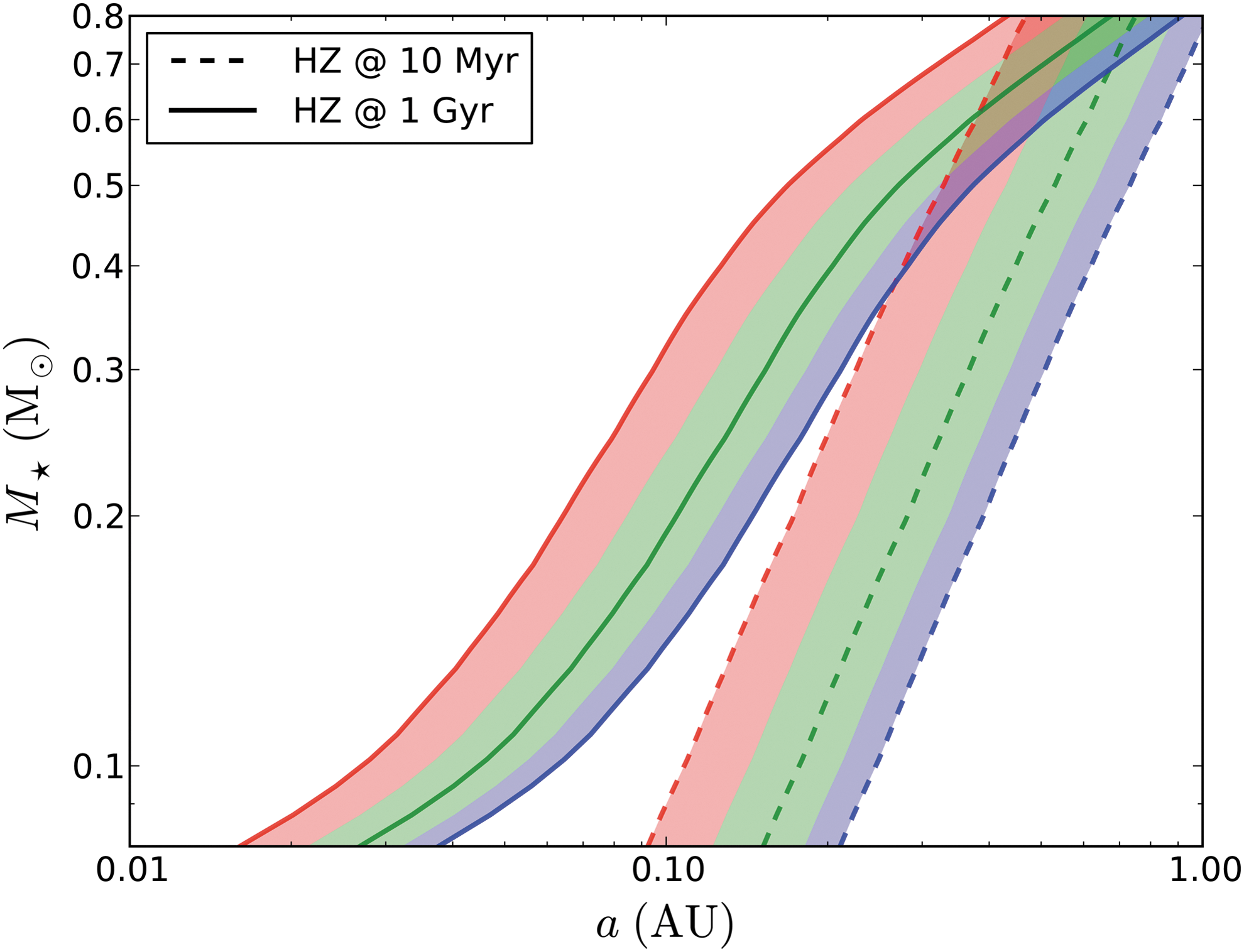
Location of the inner habitable zone (red), central habitable zone (green), and outer habitable zone (blue) as a function of stellar mass at 10 Myr (dashed) and 1 Gyr (solid). After 1 Gyr, the evolution of the HZ is negligible for M dwarfs.
Finally, we note that the location of the HZ is also a function of the eccentricity e. This is due to the fact that at a fixed semimajor axis a, the orbit-averaged flux 〈F
bol〉 is higher for more eccentric orbits (Williams and Pollard, 2002):
2.3. Atmospheric mass loss
Planetary atmospheres constantly evolve. Several mechanisms exist through which planets can lose significant quantities of their atmospheres to space, leading to dramatic changes in composition and in some cases complete atmospheric erosion. Early Earth itself could have been rich in hydrogen, with mixing ratios as high as 30% in the prebiotic atmosphere (Tian et al., 2005; Hashimoto et al., 2007). A variety of processes subsequently led to the loss of most of this hydrogen; Watson et al. (1981) argued that on the order of 1023 g of hydrogen could have escaped in the first billion years. Similarly, Kasting and Pollack (1983) calculated that early Venus could have lost an Earth ocean equivalent of water in the same amount of time. Currently, observational evidence for atmospheric escape exists for two “hot Jupiters,” HD 209458b (Vidal-Madjar et al., 2003) and HD 189733b (Lecavelier des Etangs et al., 2010), and one “hot Neptune,” GJ 436b (Kulow et al., 2014), whose proximity to their parent stars leads to the rapid hydrodynamic loss of hydrogen.
Atmospheric escape mechanisms fall into two major categories: thermal escape, in which the heating of the upper atmosphere accelerates the gas to velocities exceeding the escape velocity, and nonthermal escape, which encompasses a variety of mechanisms and may involve energy exchange among ions or erosion due to stellar winds. While nonthermal processes certainly do play a role in the evaporation of super-Earth and mini-Neptune atmospheres, the high exospheric temperatures resulting from strong XUV irradiation probably make thermal escape the dominant mechanism for planets around M dwarfs at early times. However, the escape can be greatly enhanced by flares and coronal mass ejections, which can completely erode the atmosphere of a planet lacking a strong magnetic field (Lammer et al., 2007; Scalo et al., 2007). For a review of the nonthermal mechanisms of escape, the reader is referred to Hunten (1982).
2.3.1. Jeans escape
In the low temperature limit, atmospheric mass loss occurs via the ballistic escape of individual atoms from the collisionless exosphere, where the low densities ensure that atoms with outward velocities exceeding the escape velocity will escape the planet. Originally developed by Jeans (1925), who assumed a hydrostatic, isothermal atmosphere, the mass loss rate of a pure hydrogen atmosphere is given by (Öpik, 1963)
where R
exo is the radius of the exobase, n is the number density of hydrogen atoms at the exobase, m
H is the mass of a hydrogen atom, v
t is the thermal velocity of the gas, and λJ is the Jeans escape parameter, defined as the ratio of the potential energy to the kinetic energy of the gas and given by
where G is the gravitational constant, M p is the mass of the planet, and T exo is the temperature in the (isothermal) exosphere. Since in the Jeans regime the thermal velocity of the gas is less than the escape velocity, the bulk of the gas remains bound to the planet, and only atoms in the tail of the Maxwell-Boltzmann distribution are able to escape. Jeans escape is thus slow. As an example, the present Jeans escape flux for hydrogen on Venus is on the order of 10 cm−2 s−1 (Lammer et al., 2006), corresponding to the feeble rate of ∼10−4 g/s, which would remove only one part in 1011 of the atmosphere per billion years.
For higher exospheric temperatures and/or larger values of R exo, however, corresponding to low values of λJ, the atmosphere enters a regime in which the velocity of the average atom in the exosphere approaches the escape velocity of the planet. In this regime, the bulk of the upper atmosphere ceases to be hydrostatic (and isothermal), (4) is no longer valid, and the escape rate must be calculated from hydrodynamic models.
2.3.2. Hydrodynamic escape
One of the primary mechanisms for heating the exosphere and decreasing λJ is via strong XUV irradiation. XUV photons are absorbed close to the base of the thermosphere, where they deposit energy and heat the gas via the ionization of atomic hydrogen. This heating is balanced by the adiabatic expansion of the upper atmosphere, downward heat conduction, and cooling by recombination radiation. For sufficiently high XUV fluxes, the expansion of the atmosphere accelerates the gas to supersonic speeds, at which point a hydrodynamic wind is established similar to the solar Parker wind (Parker, 1965). Once the gas reaches the exosphere, it will escape the planet provided its kinetic energy exceeds the energy required to lift it out of the planet's gravitational well.
Since the kinetic energy of a hydrogen atom at the exobase is
Originally proposed by Watson et al. (1981), the energy-limited model assumes that the XUV flux is absorbed in a thin layer at radius R
XUV where the optical depth to stellar XUV photons is unity. Recently updated to include tidal effects by Erkaev et al. (2007), this model approximates the mass loss as
where ε
XUV is the heating efficiency parameter (see below), F
XUV is the incident XUV flux, R
p is the planet radius, and K
tide is a tidal enhancement factor, accounting for the fact that for sufficiently close-in planets, the stellar gravity reduces the gravitational binding energy of the gas such that it need only reach the Roche radius to escape the planet. Erkaev et al. (2007) showed that
where the parameter ξ is defined as
with
where M ⋆ is the mass of the star and a is the semimajor axis. For simplicity, as in the work of Lopez et al. (2012), we replace R p with R XUV in (5), which is approximately valid given that R XUV is typically only 10–20% larger than R p (Murray-Clay et al., 2009; Lopez et al., 2012).
Since the input XUV energy is balanced in part by cooling radiation (via Lyman α emission in the case of hydrogen) and heat conduction, only a fraction of it goes into the adiabatic expansion that drives escape. Rather than running complex hydrodynamic and radiative transfer models to determine the net heating rate, many authors (Jackson et al., 2010; Leitzinger et al., 2011; Lopez et al., 2012; Koskinen et al., 2013; Lammer et al., 2013) choose to fold the balance between XUV heating and cooling into an efficiency parameter, ε XUV, defined as the fraction of the incoming XUV energy that is converted into PdV work. Because of the complex dependence of ε XUV on the atmospheric composition and structure, its value is still poorly constrained. Lopez et al. (2012) estimated ε XUV=0.2±0.1 for super-Earths and mini-Neptunes based on values found throughout the literature. Earlier work by Chassefière (1996) estimates ε XUV≲0.30 for Venus-like planets, but the author argues that the actual value may be closer to 0.15. Recently, Owen and Jackson (2012) found X-ray efficiencies ≲0.1 for planets more massive than Neptune, but higher efficiencies (∼0.15) for terrestrial planets. Moreover, Shematovich et al. (2014) argued that studies that assume efficiencies higher than about 0.2 probably lead to overestimates in the escape rate. On the other hand, some studies suggest higher heating efficiencies: Koskinen et al. (2013) used hydrodynamic and photochemical models of the hot Jupiter HD 209458b to calculate ε XUV=0.44.
As we have already implied, unlike Jeans escape, hydrodynamic blow-off is fast. Chassefière (1996) calculated the maximum hydrodynamic escape rate from the early venusian atmosphere to be ∼106 g/s, 10 orders of magnitude higher than the present Jeans escape flux (see Section 2.3.1). Although there has been debate over the validity of the blow-off assumption (see, for instance, the discussion in Tian et al., 2008), recently Lammer et al. (2013) showed that, for super-Earths exposed to high levels of XUV irradiation, the energy-limited approximation yields mass loss rates that are consistent with hydrodynamic models to within a factor of about 2, which is within the uncertainties of the problem.
2.3.3. Controlled hydrodynamic escape
It is also worth noting that there may be an intermediate regime between Jeans escape and blow-off known as “modified Jeans escape” or “controlled hydrodynamic escape” (Erkaev et al., 2013). In this regime, which occurs for intermediate XUV fluxes and/or higher planetary surface gravity, blow-off conditions are not met, but the atmosphere still expands, so that the hydrostatic Jeans formalism is not valid. To calculate the escape rate, one must replace the classical Maxwellian velocity distribution with one that includes the bulk expansion velocity of the atmosphere. This yields escape rates lower than those due to a hydrodynamic flow but significantly higher than those predicted by the hydrostatic Jeans equation (3).
2.3.4. Jeans escape or hydrodynamic escape
Since the location of the HZ is governed primarily by the total (bolometric) flux incident on a planet, the higher ratio of L XUV to L bol of M dwarfs implies a much larger XUV flux in the HZ compared to solar-type stars. The present-day solar XUV luminosity is L XUV/L bol≈3.4×10⁻⁶ (see Table 4 in Ribas et al., 2005), while for active M dwarfs this ratio is ∼10−3 (e.g., Scalo et al., 2007). Therefore, we should expect planets in the HZ of M dwarfs to experience XUV fluxes several orders of magnitude greater than the present Earth level (F XUV ⊕≈4.64 erg/s/cm2). Recent papers (Lammer et al., 2007, 2013; Erkaev et al., 2013) show that terrestrial planets experiencing XUV fluxes corresponding to 10× and 100×F XUV ⊕ are in the hydrodynamic flow regime, and we may thus expect the same for super-Earths/mini-Neptunes in the HZ of active M dwarfs.
In Fig. 2, we plot the evolution of the XUV flux received by a planet located close to the inner edge of the HZ (defined at 5 Gyr) for three different M dwarf masses and two different XUV saturation times (see Section 2.1). The dashed lines correspond to the critical fluxes in the work of Erkaev et al. (2013) above which hydrodynamic escape occurs, for 1 and 10 M ⊕ and two values of ε XUV. Earth-mass planets remain in the hydrodynamic escape regime for at least 1 Gyr in all cases and in excess of 10 Gyr for active M dwarfs. The duration of this regime is shorter for 10 M ⊕ planets but still on the order of several 100 Myr.
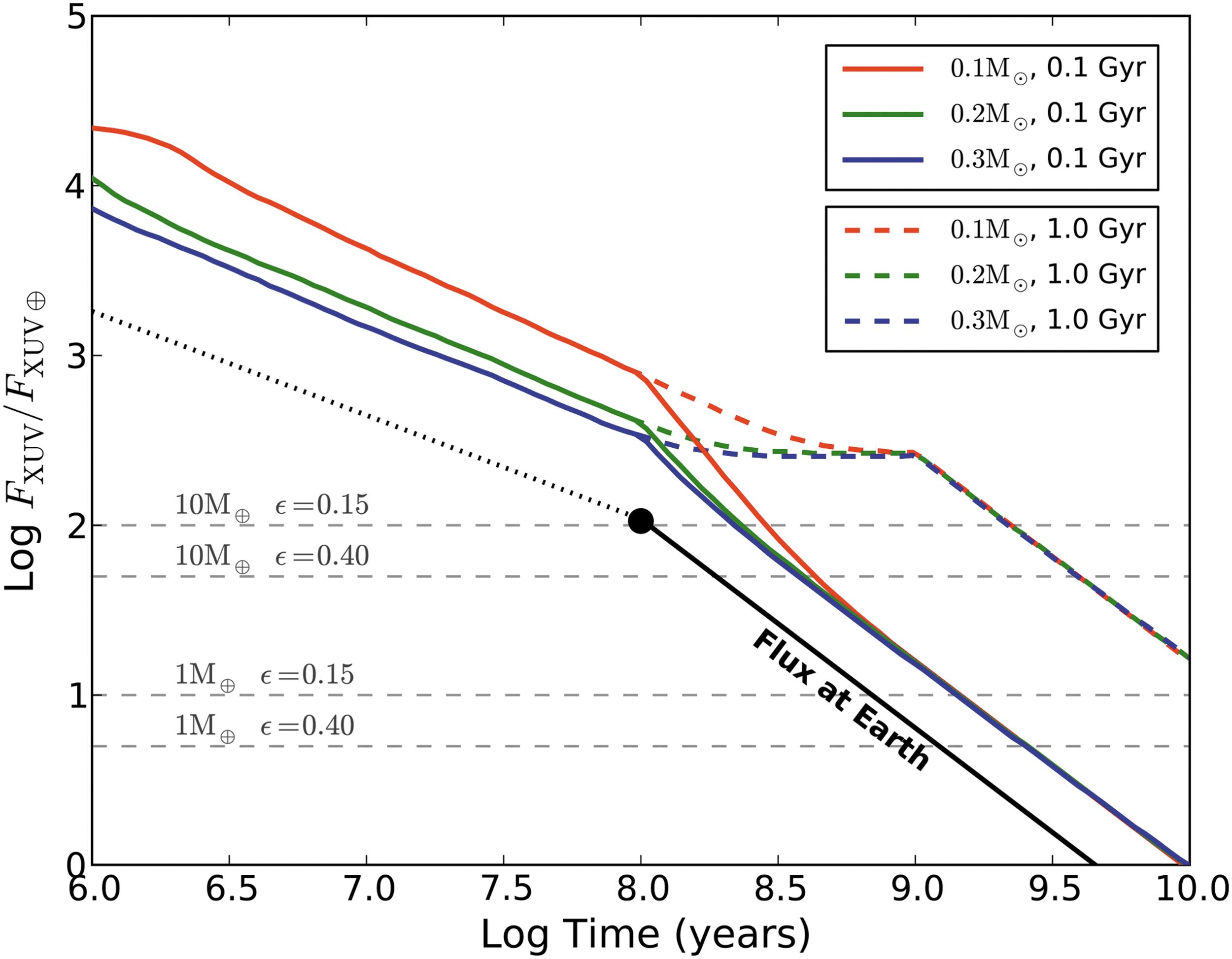
Evolution of the XUV flux received by planets close to the inner edge of the HZ (at 1 Gyr) for stars of mass 0.1, 0.2, and 0.3 M ⊙. Solid lines correspond to an XUV saturation time of 0.1 Gyr; dashed lines correspond to 1 Gyr. The flux at Earth is indicated by the black line. The dot corresponds to the earliest time for which Ribas et al. (2005) had data for solar-type stars; this is also roughly the time at which Earth formed. An XUV luminosity saturated at 10−3 L bol is roughly indicated by the dotted line. Finally, the dashed gray lines indicate the minimum XUV fluxes required to sustain blow-off according to the study of Erkaev et al. (2013). Super-Earths in the HZs of M dwarfs remain in the blow-off regime for at least a few 100 Myr; Earths undergo blow-off for much longer. For an XUV saturation time of 1 Gyr, blow-off occurs for several billion years for all planets.
We note also that tidal effects can significantly increase the critical value of λ
J below which hydrodynamic escape occurs (see discussion in Erkaev et al., 2007). Hydrodynamic escape ensues when the thermal energy of the gas exceeds its potential energy, which occurs when
or
provided we maintain the original definition of the Jeans parameter (4). Due to the strong tidal forces acting on the planets we consider here, this effect should greatly increase the critical value of the escape parameter, effectively reducing the value of F XUV for which hydrodynamic escape occurs.
2.3.5. Energy-limited or radiation/recombination-limited?
Hydrodynamic escape from planetary atmospheres need not be energy-limited. In the limit of high extreme ultraviolet (EUV) flux (low-energy XUV photons with 100 Å≲λ≲1000 Å), Murray-Clay et al. (2009) showed that the escape is “radiation/recombination-limited,” scaling roughly as
where r
s is the radius of the sonic point (where the wind velocity equals the local sound speed c
s) and ρ
s is the density at r
s. Since the bulk of the flow is ionized, the density is fixed by ionization-recombination balance, scaling roughly as (F
EUV
r
s)1/2. For a 0.7 M
J hot Jupiter, the radiation/recombination-limited mass loss rate is (Murray-Clay et al., 2009)
Owen and Jackson (2012) re-derived this expression with explicit scalings on several planetary properties:
where the quantity (1+x) is the radius of the ionization front in units of R
p, f
parker is the Mach number of the flow, Φ
★ is the stellar EUV luminosity in photons per second, A is a geometrical factor, and c
EUV is the isothermal sound speed of the gas. Taking x=0, f
parker=1, A=1/3, c
EUV=10 km/s, and an average EUV photon energy hν=20 eV, this becomes
The transition from energy-limited to radiation/recombination-limited escape is found by equating the two expressions, namely, (5) and (13), and solving for the critical EUV flux. For hot Jupiters and mini-Neptunes alike, the transition occurs at roughly F EUV∼104 erg/cm2/s. Below this flux, the escape is energy-limited; above it, the escape is radiation/recombination-limited and thus increases more slowly with the flux.
Mini-Neptunes that migrate early into the HZ of M dwarfs are exposed to EUV fluxes up to an order of magnitude larger than this critical value. During this period, which lasts on the order of a few hundred million years, the mass loss rate may be radiation/recombination-limited.
However, whether the high-flux mass loss rate is more accurately described by (5) or (13) will depend on whether the flux is dominated by X-ray or EUV radiation. Owen and Jackson (2012) showed that the mass loss rate for X-ray-driven hydrodynamic winds scales linearly with the X-ray flux; this is because the sonic point for X-ray flows tends to occur below the ionization front. Even though recombination radiation still removes energy from the flow, it does so once the gas is already supersonic and thus causally decoupled from the planet, such that it cannot bottleneck the escape. Although the authors caution that the dependence of the mass loss rate on planet mass and radius must be determined numerically, this regime is analogous to the energy-limited regime and can be roughly approximated by (5).
For X-ray luminosities L X≳10−6 L ⊙, close-in planets undergo X-ray driven hydrodynamic escape (see Fig. 11 in Owen and Jackson, 2012). If X-rays contribute significantly to the XUV emissions of young M dwarfs, their X-ray luminosities may exceed this value for as long as 1 Gyr, and close-in mini-Neptunes will undergo energy-limited escape. Unfortunately, given the lack of observational constraints on the X-ray/EUV luminosities of young M dwarfs, it is unclear at this point whether the hydrodynamic escape will be EUV-driven (radiation/recombination-limited) or X-ray-driven (energy-limited).
2.3.6. The effect of eccentricity
Most of the formalism that has been developed to analytically treat hydrodynamic blow-off only considers circular orbits. For planets on sufficiently eccentric orbits, neither the stellar flux nor the tidal effects may be treated as constant over the course of an orbit. Due to this fact, an expression analogous to (5) for eccentric orbits seems to be lacking in the literature. In this section, we derive such an expression.
There are two separate effects that enhance the mass loss for planets on eccentric orbits. Most papers account for the first effect, which is the increase of the orbit-averaged stellar flux by a factor of 1/
One might wonder whether this replacement is valid. Specifically, if R Roche(t) changes faster than the atmosphere is able to respond to the changes in the gravitational potential, we would expect that the time dependence of the mass loss rate would be a complicated function of the tides generated in the atmosphere. On the other hand, if the orbital period is very large compared to the dynamical timescale of the planet, the atmosphere will have sufficient time to assume the equilibrium shape dictated by the new potential. This limit is known as the quasi-static approximation (Sepinsky et al., 2007). In the Appendix, we show that all the planets in our runs with eccentricities e≲0.4 are in the quasi-static regime and that (14) is therefore valid. In some runs, we allow the eccentricity to increase beyond 0.4. We discuss the implications of this in Section 5.9.
Since R
Roche=R
Roche(t), ξ, K
tide, and dM/dt (Eqs. 5, 6, and 7) are now also functions of t, varying significantly over a single orbit. To account for this, we may calculate the time-averaged mass loss rate over the course of one orbit,
where ξ is the time-independent parameter given by (7) and (8), and E is the eccentric anomaly. The average mass loss rate is then simply
where
is the zero-eccentricity mass loss rate in the absence of tidal enhancement. Note that the flux-enhancement factor
For ξ≳10, the integral may be approximated by the analytic expression
which greatly reduces computing time.
As we show in the Appendix, the decreased Roche lobe distance for eccentric orbits has a large effect on the amount of mass lost, particularly for low values of ξ and for high e (see Fig. A2). Moreover, higher eccentricities result in RLO at larger values of a compared to the circular case, since the planet may overflow near pericenter, leading to mass loss rates potentially orders of magnitude higher. We discuss RLO in detail in the Model Description section (Section 3.3).
2.4. Tidal theory
The final aspect of planetary evolution we discuss is the effect of tidal interactions with the host star. Below we review two different approaches to analytically calculate the orbital evolution of the system.
2.4.1. Constant phase lag
Classical tidal theory predicts that torques arising from interactions between tidal deformations on a planet and its host star lead to the secular evolution of the orbit and the spin of both bodies. In this paper, we employ the “equilibrium tide” model of Darwin (1880), which approximates the tidal potential as a superposition of Legendre polynomials representing waves propagating along the surfaces of the bodies; these add up to give the familiar tidal “bulge.” Because of viscous forces in the bodies' interiors, the tidal bulges do not instantaneously align with the line connecting the two bodies. Instead, the N
th wave on the i
th body will lag or lead by an angle ɛN,i
, assumed to be constant in the constant phase lag (CPL) model. In general, different waves may have different lag angles, and it is unclear how the ɛN,i
vary as a function of frequency. A common approach (see Ferraz-Mello et al., 2008) is to assume that the magnitudes of the lag angles are equal (see Goldreich and Soter, 1966), while their signs may change depending on the orbital and rotational frequencies involved. This allows us to introduce the tidal quality factor
which in turn allows us to express the lags (in radians) as
The parameter Qi is a measure of the dissipation within the i th body; it is inversely proportional to the amount of orbital and rotational energy lost to heat per cycle, in analogy with a damped-driven harmonic oscillator. The merit of this approach is that the tidal response of a body can be captured in a single parameter. Planets with high values of Q p have smaller phase lags, dissipate less energy, and undergo slower orbital evolution; planets with low values of Q p have larger phase lags, higher dissipation rates, and therefore faster evolution. Measurements in the Solar System constrain the value of Q p for terrestrial bodies in the range 10–500, while gas giants are consistent with Q p∼104 to 105 (Goldreich and Soter, 1966). Values of Q ★ for the Sun and other main sequence stars are poorly constrained but are likely to be ≳105 to 106 (Schlaufman et al., 2010; Penev et al., 2012). Intuitively, this makes sense, given that the dissipation due to internal friction in rocky bodies should be much higher than that in bodies dominated by gaseous atmospheres. One should bear in mind, however, that the exact dependence of Qi on the properties of a body's interior is likely to be extremely complicated. Given the dearth of data on the composition and internal structure of exoplanets, it is at this point impossible to infer precise values of Q p for these planets.
By calculating the forces and torques due to the tides raised on both the planet and the star, one can arrive at the secular expressions for the evolution of the planet's orbital parameters, which are given by a set of coupled nonlinear differential equations; these are reproduced in the Appendix.
2.4.2. Constant time lag
Unlike the CPL model, which assumes the phase lag of the tidal bulge is constant, the constant time lag (CTL) model assumes that it is the time interval between the bulge and the passage of the perturbing body that is constant. Originally proposed by Alexander (1973) and updated by Leconte et al. (2010), this model allows for a continuum of tidal wave frequencies and therefore avoids unphysical discontinuities present in the CPL model. However, implicit in the CTL theory is the assumption that the lag angles are directly proportional to the driving frequency (Greenberg, 2009), which is likely also an oversimplification. We note, however, that in the low eccentricity limit, both the CPL and the CTL models arrive at qualitatively similar results. At higher eccentricities, the CTL model is probably better suited, given that it is derived to eighth order in e (versus second order in the CPL model).
The tidal quality factors Qi
do not enter the CTL calculations at any point; instead, the dissipation is characterized by the time lags τi
. Although there is no general conversion between Qi
and τi
, Leconte et al. (2010) showed that provided annual tides dominate the evolution,
where n is the mean motion (or the orbital frequency) of the secondary body (in this case, the planet).
For a planet with Q p=104 in the center of the HZ of a late M dwarf, τ p≈10 s; rocky planets with lower Q p may have values on the order of hundreds of seconds. Since τ∝n −1, close-in planets should have much lower time lags. For reference, Leconte et al. (2010) argued that hot Jupiters should have 2×10⁻³ s≲τ p≲2×10⁻² s.
The tidal evolution expressions are reproduced in the Appendix. For a more detailed review of tidal theory, the reader is referred to Ferraz-Mello et al. (2008), Heller et al. (2011), and the appendices in Barnes et al. (2013).
3. Model Description
Our model evolves planet-star systems forward in time in order to determine whether HECs can form from mini-Neptunes that have migrated into the HZs of M dwarfs. We perform our calculations on a grid of varying planetary, orbital, and stellar properties to determine the types of systems that may harbor HECs. The complete list is provided in Table 1, where we indicate the ranges of values we consider as well as the default values adopted in the plots in Section 4 (unless otherwise indicated).
Integrations are performed from t=t 0 (the time at which the planet is assumed to have migrated into the HZ) to t=t stop (the current age of the system) with the adaptive timestepping method described in Appendix E of Barnes et al. (2013).
3.1. Stellar model
We use the evolutionary tracks of Baraffe et al. (1998) for solar metallicity to calculate L bol and T eff as a function of time. We then use (1) to calculate L XUV, given (L XUV/L bol)sat=10−3 and values of t sat and β given in Table 1.
Using L bol and T eff, we calculate the location of the HZ from the equations given by Kopparapu et al. (2013), adding the eccentricity correction (2). Given the uncertainty in the actual HZ boundaries and their dependence on a host of properties of a planet's climate, we choose our inner edge of the habitable zone (IHZ) to be the average of the Recent Venus and the Runaway Greenhouse limits and our outer edge of the habitable zone (OHZ) to be the average of the Maximum Greenhouse and the Early Mars limits. Throughout this paper, we will also refer to the center of the habitable zone (CHZ), which we take to be the average of the IHZ and OHZ. Since we are concerned with the formation of ultimately habitable planets, we take the locations of the IHZ, CHZ, and OHZ to be their values at 1 Gyr, at which point the stellar luminosity becomes roughly constant.
3.2. Planet radius model
To determine the planet radius R p as a function of the core mass M c, the envelope mass fraction f H≡M e/M p, and the planet age, we use the planet structure model described by Lopez et al. (2012) and Lopez and Fortney (2014), which is an extension of the model of Fortney et al. (2007) to low-mass low-density (LMLD) planets. These models perform full thermal evolution calculations of the interior as a function of time. In our runs, the core is taken to be Earth-like, with a mixture of two-thirds silicate rock and one-third iron, and the envelope is modeled as a H/He adiabat. A grid of values of R p is then computed in the range 1 M ⊕≤M c≤10 M ⊕, 10−6≤f H≤0.5, and 107 years≤t≤1010 years. For values between grid points, we perform a simple trilinear interpolation. For gas-rich planets, R p is the 20 mbar radius; for gas-free planets, it corresponds to the surface radius. The evolution of R p with age due solely to thermal contraction is plotted in Fig. 3 for a few different planet masses and values of f H.
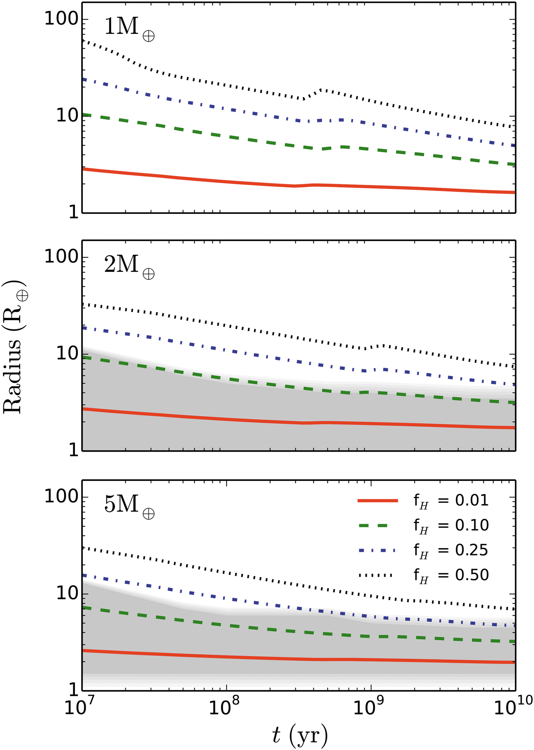
Evolution of the radius as a function of time due to thermal contraction of the envelope, in the absence of tidal effects and atmospheric mass loss. From top to bottom, the plots correspond to planets with initial total masses (core+envelope) of 1, 2, and 5 M ⊕. Line styles correspond to different initial hydrogen mass fractions: 1% (red, solid), 10% (green, dashed), 25% (blue, dot-dashed), and 50% (black, dotted). For comparison, the gray shaded regions in the bottom two plots are the spread in radii calculated by Mordasini et al. (2012b) for f H≲0.20. See text for a discussion.
We note that the models of Fortney et al. (2007) and Lopez et al. (2012) are in general agreement with those of Mordasini et al. (2012a, 2012b) and, by extension, Rogers et al. (2011). Mordasini et al. (2012a) presented a validation of their model against that of Fortney et al. (2007), showing that for planets spanning 0.1 to 10 Jupiter masses, the two models predict the same radius to within a few percent. At the lower masses relevant to our study, the two models are also in agreement. To demonstrate this, in Fig. 3 we shade the regions corresponding to the spread in radii at a given mass and age in Fig. 9 of Mordasini et al. (2012b). Since those authors used a coupled formation/evolution code, at low planet mass the maximum envelope mass fraction f H is small; for a total mass of 4 M ⊕, Mordasini et al. (2012b) found that all planets have f H<0.2. At 2 M ⊕, most planets have f H≲0.1. We can see from Fig. 3 that at these values of f H, the two models predict very similar radius evolution. Note that Mordasini et al. (2012b) did not consider planets less massive than 2 M ⊕.
The maximum envelope fraction merits further discussion. Since we do not model the formation of mini-Neptunes, we do not place a priori constraints on the value of f H at a given mass; instead, we allow it to vary in the range 10−6≤f H≤0.5 for all planet masses. At masses ≲5 M ⊕, planets accumulate gas slowly and are typically unable to accrete more than ∼10–20% of their mass in H/He (Rogers et al., 2011; Bodenheimer and Lissauer, 2014); values of f H≈0.5 may thus be unphysical. However, as we argue in Section 5.1, the longer disk lifetimes around M dwarfs (Carpenter et al., 2006; Pascucci et al., 2009) allow more time for gas accretion, potentially increasing the maximum value of f H. Nevertheless, and more importantly, if a planet with f H=0.5 loses its entire envelope via atmospheric escape, any planet with the same core mass and f H<0.5 will also lose its envelope. Below, where we present integrations with f H=0.5, our results are therefore conservative, as planets with f H <<0.5 will in general evaporate more quickly.
While our treatment of the radius evolution is an improvement upon past tidal-atmospheric coupling papers (Jackson et al., 2010, for instance, calculated R p for super-Earths by assuming a constant density as mass is lost), there are still issues with our approach, as follows: (1) We do not account for inflation of the radius due to high insolation. Instead, we calculate our radii from grids corresponding to a planet receiving the same flux as Earth. While at late times this is justified, since planets in the HZ by definition receive fluxes similar to Earth, at early times this is probably a poor approximation; recall that planets in the HZ around low-mass M dwarfs are exposed to fluxes up to 2 orders of magnitude higher during the host star's PMS phase. The primary effect of a higher insolation is to act as a blanket, delaying the planet's cooling and causing it to maintain an inflated radius for longer. This will result in mass loss rates higher than what we calculate here. (2) Since we are determining the radii from pre-computed grids, we also do not model the effect of tidal dissipation on the thermal evolution of the planet. Planets undergoing fast tidal evolution can dissipate large amounts of energy in their interiors, which should lead to significant heating and inflation of their radii. (3) The radius is also likely to depend on the mass loss rate. Setting R p equal to the tabulated value for a given mass, age, and composition is valid only as long as the timescale on which the planet is able to cool is significantly shorter than the mass loss timescale. Otherwise, the radius will not have enough time to adjust to the rapid loss of mass, and the planet will remain somewhat inflated, leading to a regime of runaway mass loss (Lopez et al., 2012). While the planets considered here are probably not in the runaway regime [Lopez et al. (2012) found that runaway mass loss occurred only for H/He mass fractions ≳90%], we might still be significantly underestimating the radii during the early active phase of the parent star.
All points outlined above lead to an underestimate of the radius at a given time. Since the mass loss rate is proportional to
3.3. Atmospheric escape model
We assume that the escape of H/He from the planetary atmosphere is hydrodynamic (blow-off) at all times, which is valid at the XUV fluxes we consider here (see Erkaev et al., 2013, and Fig. 2). We run two separate sets of integrations: one in which we assume the flow is energy-limited (5) for all values of F XUV, and one in which we switch from energy-limited to radiation/recombination-limited (13) above the critical value of the flux (see Section 2.3.5). For planets whose orbits are eccentric enough that they switch between the two regimes over the course of one orbit, we make use of the expressions derived in Section A.3 in the Appendix. These two sets of integrations should roughly bracket the true mass loss rate.
For eccentric orbits, we calculate the mass loss in the energy-limited regime from (16), with K ecc evaluated from (15). We vary ε XUV and R XUV in the ranges given in Table 1. We choose ε XUV=0.30 as our default case. While this is consistent with values cited in the literature (see Section 2.3.2), it could be an overestimate. We discuss the implications of this choice in Section 5.3.
Given the large planetary radii at early times, many of the planets we model here are not stable against RLO in the HZ. During RLO, the stellar gravity causes the upper layers of the atmosphere to suddenly become unbound from the planet; this occurs when R p>R Roche, where R Roche is given by (8). For a planet that forms and evolves in situ, RLO never occurs, since any gas that would be lifted from the planet in this fashion would have never accreted in the first place. However, an inflated gaseous planet that forms at a large distance from the star may initially be stable against overflow and enter RLO as it migrates inward (since R Roche∝a). This is particularly the case for planets in the HZs of M dwarfs, since a and consequently R Roche are small.
Ideally, the tidally enhanced mass loss rate equation (5) should capture this process, but instead it predicts an infinite mass loss rate as R XUV→R Roche (or as ξ→1) and unphysically changes sign for ξ<1. This is due to the fact that the energy-limited model implicitly assumes that the bulk of the atmosphere is located at R XUV (the single-layer assumption). Realistically, we would expect the planet to quickly lose any mass above the Roche lobe and then return to the stable hydrodynamic escape regime. However, upon loss of the material above R Roche, the portion of the envelope below the new XUV absorption radius R′ XUV will not be in hydrostatic equilibrium; instead, an outward flow will tend to redistribute mass to the evacuated region above, leading to further overflow.
Several models exist that allow one to calculate the mass loss rate due to RLO (e.g., Ritter, 1988; Trilling et al., 1998; Gu et al., 2003; Sepinsky et al., 2007). These often involve calculating the angular momentum exchange between the outflowing gas and the planet, which can lead to its outward migration, given by
for a planet on a circular orbit (Gu et al., 2003; Chang et al., 2010). This leads to a corresponding increase in R Roche until it reaches R XUV and the overflow is halted. By differentiating the stability criterion R XUV(M p)=R Roche(M p), one may then obtain an approximate expression for dM p/dt in terms of the density profile dM(<R)/dR of the envelope.
However, for mini-Neptunes that migrate into the HZ early on, RLO should occur during the initial migration process, which we do not model in this paper. Instead, we begin our calculations by assuming that our planets are stable to RLO in the HZ. If a planet's radius initially exceeds the Roche lobe radius, we set its envelope mass equal to the maximum envelope mass for which it can be stable at its current orbit; the difference between the two envelope masses is the amount of H/He it must have lost prior to its arrival in the HZ. It is important to note that these planets will initially have R
XUV=R
Roche, which, as we mentioned above, leads to an infinite mass loss rate in (5). An accurate determination of
In Fig. 4 we show how the time t
evap at which complete evaporation takes place scales with ξ
min for a typical mini-Neptune in the IHZ (red), CHZ (green), and OHZ (blue). Also plotted is the mass loss enhancement factor 1/K
tide (Eq. 6, black dashed line) as a function of ξ=ξ
min. Interestingly, despite the fact that the instantaneous mass loss rate (
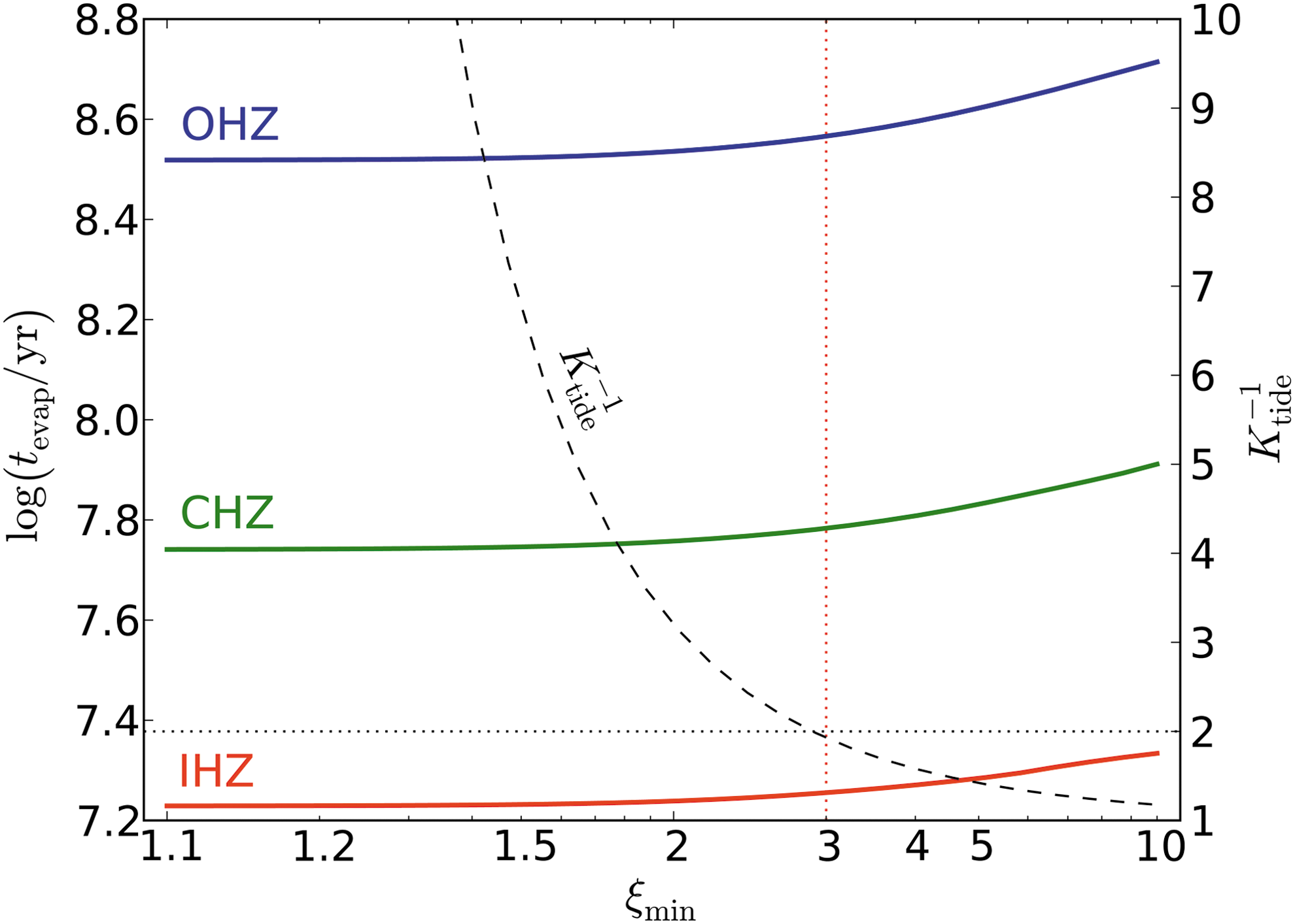
Complete evaporation time t evap as a function of the cutoff value ξ min for a 2 M ⊕ mini-Neptune with initial f H=0.5 on a circular orbit around a 0.08 M ⊙ star. The red, green, and blue lines correspond to planets in the IHZ, CHZ, and OHZ, respectively. Also plotted is the mass loss enhancement factor 1/K tide (black dashed line), which approaches infinity as ξ→1. Note that for ξ min≲3, the evaporation time is relatively insensitive to the exact cutoff value, despite the fact that 1/K tide blows up. We therefore choose ξ min=3 as the default cutoff, corresponding to a maximum enhancement factor 1/K tide≈2.
3.4. Tidal model
We calculate the evolution of the semimajor axis, the eccentricity, and the rotation rates from (60)–(62) and (73)–(75) in the Appendix for the CPL and CTL models, respectively. For simplicity, we set the obliquities of all our planets to zero. Since the tidal locking timescale is very short for close-in planets 1 (Gu et al., 2003), we assume that the planet's rotation rate is given by the equilibrium value (65) or (78).
We calculate the stellar spin by assuming different initial periods (see Table 1) and evolving it according to the tidal equations, while enforcing conservation of angular momentum as the star contracts during the PMS phase. We neglect the effects of rotational braking (Skumanich, 1972), whereby stars lose angular momentum to winds and spin down over time. This leads to an overestimate of the spin rate at later times, but tidal effects should only be important early on, when the radii and the eccentricity are higher. Bolmont et al. (2012) recently modeled the coupling between stellar spin and tides, following the evolution of a “slow rotator” star (P 0≈10 days) and a “fast rotator” star (P 0≈1 day). In both cases, the stars sped up during the first ∼300–500 Myr, after which time angular momentum loss became significant. However, tidal evolution is orders of magnitude weaker at such late times, so we would expect rotational braking to have a minimal effect on the tidal evolution. Moreover, as we show in the Appendix, in general it is the tide raised on the planet that dominates the evolution; as this depends on the planetary rotation rate, and not on the stellar rotation rate, our results are relatively insensitive to the details of the spin evolution of the star.
In the CPL model, we adopt typical gas giant values 104≤Q p≤105 for gas-rich mini-Neptunes and typical terrestrial values 10≤Q p≤500 for planets that have lost their envelopes; we assume stellar values in the range 105≤Q ★≤106. In the CTL model, we consider time lags in the range 10−3 s≤τ p≤101 s for gas-rich mini-Neptunes and 10−1 s≤τ p≤103 s once they lose their envelopes. Following Leconte et al. (2010), we consider stellar time lags in the range 10−2 s≤τ ★≤10−1 s.
Once a mini-Neptune loses all its atmosphere, we artificially switch Q p or τ p to the terrestrial value adopted in that run. In reality, as the atmosphere is lost, the transition from high to low Q p (or low to high τ p) should be continuous. A detailed treatment of the dependence of Q p and τ p on the envelope mass fraction is deferred to future work.
Finally, we note that the second-order CPL model described above is valid only at low eccentricity. For
4. Results
4.1. A typical run
In Fig. 5, we show the time evolution of three mini-Neptunes as a guide to understanding the results presented in the following sections. We plot planet mass and radius (top row), semimajor axis and eccentricity (center row), and stellar XUV luminosity and radius (bottom row), all as a function of time since the planet's initial migration, t 0, for 5 Gyr. In the center plots, the post-1 Gyr OHZ and CHZ are shaded blue and green, respectively. At t=t 0, the planet is a 1 M ⊕ core with a 1 M ⊕ envelope orbiting around a 0.08 M ⊙ M dwarf with e=0.5 at a semimajor axis of 0.04 AU. We set ε XUV=0.30; other parameters are equal to the default values listed in Table 1. Because of the high eccentricity, the tidal evolution is calculated according to the CTL model.
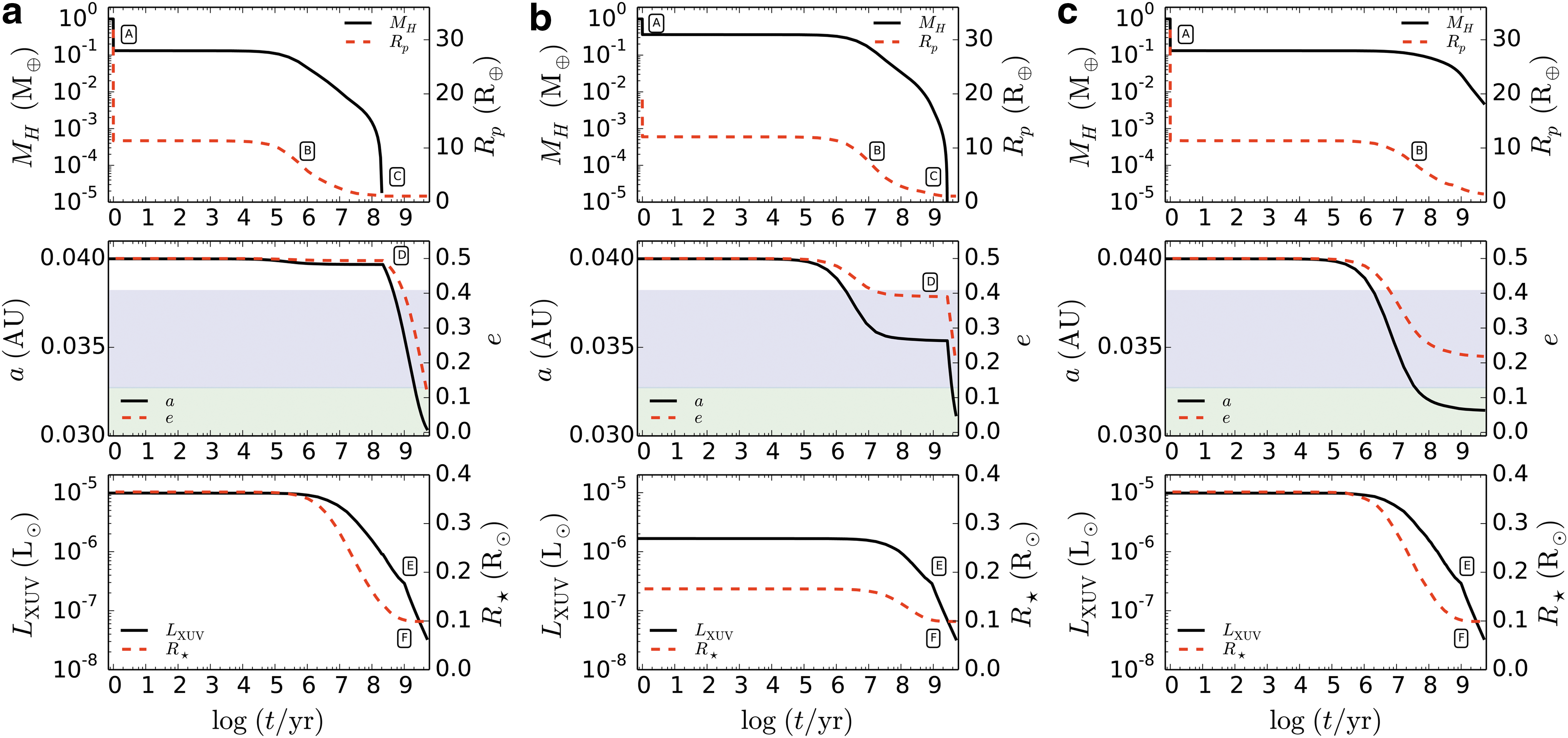
Three sample integrations of our code. The first-row plots show the envelope mass (left axis) and planet radius (right axis) versus time since formation; the second-row plots show the semimajor axis (left) and eccentricity (right) versus time; and the third row shows the stellar XUV luminosity (left) and stellar radius (right) versus time. The planet is initially a 1 M
⊕ core with a 1 M
⊕ envelope orbiting around a 0.08 M
⊙ M dwarf with e=0.5 at a semimajor axis of 0.04 AU, just outside the OHZ (light blue shading). Unless otherwise noted, all other parameters are set to their default values (Table 1). As it loses mass and tidally evolves, it migrates into the CHZ (light green shading). Note that the evolution of the HZ is not shown; the CHZ and OHZ are taken to be the long-term (>1 Gyr) values.
In column (a), we force the escape to be energy-limited (5), corresponding to an X-ray-dominated flow. Prior to the first time step, nearly 90% of the envelope mass is lost to RLO, indicated by the discontinuous drop marked
In the center plot, we see that the planet's orbit steadily decays as it circularizes, with a sharp discontinuity in the slope at ∼100 Myr (
In the bottom plot, we see that the bulk of the mass loss occurs when the stellar XUV flux is high. After t≈100 Myr, the XUV luminosity is low enough that a planet with significant hydrogen left (f
H≳0.01) is unlikely to completely evaporate. Here, the XUV saturation time is set to 1 Gyr, visible in the kink marked by the label
In column (b), we repeat the integration but delay the start time, setting t
0=100 Myr. This corresponds to a planet that undergoes a late scattering event, bringing it to a=0.04 AU when both its radius and the XUV flux are significantly smaller. In this case, RLO is somewhat less effective, removing only 50% of the envelope initially (
Finally, in column (c) we repeat the integration performed in (a), but this time set the flow to be radiation/recombination-limited above the critical flux (Section 2.3.5). Because of the significantly lower escape rate at early times, the envelope does not completely evaporate, and at 5 Gyr this is a super-Earth with slightly less than 1% hydrogen by mass. For a planet to completely lose its envelope in the radiation/recombination-limited regime, it must either migrate into an orbit closer to the star, have a larger eccentricity, have a smaller core, or be stripped by another process.
4.2. Dependence on M c, M H, M ★, and t 0
In Fig. 6, we plot the initial versus final envelope mass (M H) for planets that end up in the IHZ (red lines), CHZ (green lines), and OHZ (blue lines). Line styles correspond to different values of t 0, the time at which the planet migrated into its initial close-in orbit (solid, 10 Myr; dashed, 50 Myr; dash-dotted, 100 Myr). The colored shadings are simply an aid to the eye, highlighting the spread due to different values of t 0. For reference, in dotted gray we plot the line corresponding to a planet that undergoes no evaporation. Note that in most plots, the curves approach this line as the initial M H is increased: at constant core mass, it is in general more difficult to evaporate planets with more massive H/He envelopes. Finally, if a curve of a given color/line style is missing, the final hydrogen mass is zero for all values of the initial M H.
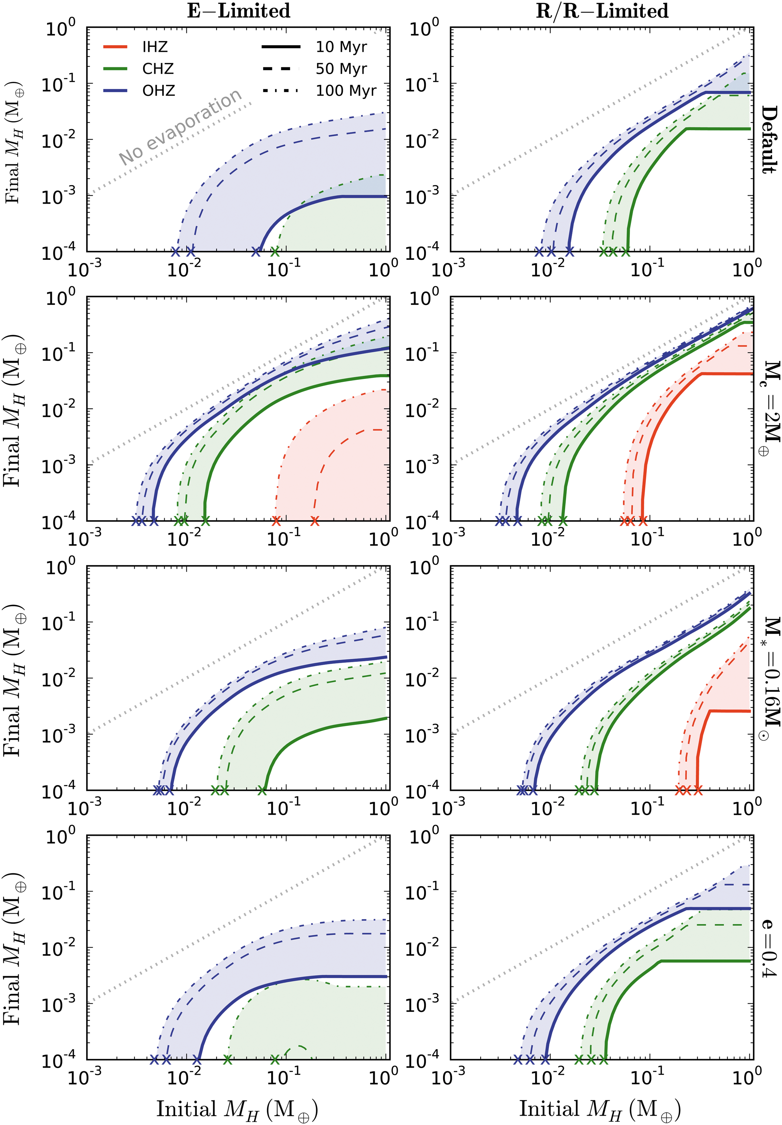
Initial versus final envelope mass (M H) for planets that end up in the IHZ (red), CHZ (green), and OHZ (blue). Line styles correspond to different values of t 0 (solid, 10 Myr; dashed, 50 Myr; dash-dotted, 100 Myr). Columns correspond to runs in which the escape mechanism is energy-limited (left) and radiation/recombination-limited (right); rows vary certain parameters as labeled, with all others set to their default values. In the default run, the planet has a 1 M ⊕ core and orbits an M dwarf with M ★=0.08 M ⊙ in a circular orbit. The dotted gray line corresponds to a planet that undergoes no evaporation. An X marks the critical initial envelope mass below which full evaporation occurs within 5 Gyr. In some plots, curves of a given color/line style are missing; for those runs, the entire envelope was lost for all starting values of M H.
The two columns correspond to runs in which the escape was forced to be energy-limited (left) and radiation/recombination-limited at high XUV flux and energy-limited at low XUV flux (right). Rows correspond to different planetary properties, as labeled. In the top (“Default”) row, the planet's core mass is set to 1 M ⊕. The planet orbits an M dwarf with M ★=0.08 M ⊙ in a circular orbit. All other parameters are set to their default values.
In the second row, we double the core mass. The third row is the same as the first but for a 0.16 M ⊙ star, and the fourth row is the same as the first but for an initial eccentricity e=0.4. Since planets in this run undergo orbital evolution, the different color curves correspond to planets that end up in the IHZ, CHZ, and OHZ, respectively (their initial semimajor axes are somewhat larger).
We first consider the general trends in the plots. For low-enough M H, all curves become nearly vertical. The critical envelope mass below which all mass is lost is marked with an X. Note that once planets lose sufficient mass such that M H≲10−4, the envelope is very unstable to complete erosion under the XUV fluxes considered here (corresponding to a near-vertical slope in this diagram). Many curves also display a flattening toward high initial envelope masses; some have prominent kinks beyond which the final envelope mass is constant. This is due to RLO, which causes any planets with radii larger than the Roche radius to lose mass prior to entering the HZ. Since increasing the envelope mass increases the planet radius, this results in a maximum envelope mass for some planets.
Planets that migrate in early (small t
0) lose significantly more mass than planets that migrate in late. This is a consequence of both the decay in the XUV luminosity of the star with time and the quick decrease of the planet radius as the planet cools. Another interesting trend is that the difference in the evaporated amount is much more pronounced in the energy-limited runs than in the radiation/recombination-limited runs. This is due to the
Now we focus on individual rows. For the default run (a 1 M ⊕ core in a circular orbit around a 0.08 M ⊙ star), all planets in the IHZ lose all their hydrogen and form HECs, regardless of migration time, envelope mass, or escape mechanism. In the CHZ, only planets that migrate within ≲50 Myr and undergo energy-limited escape form HECs for all initial values of M H. However, HECs still form from planets with M H≲0.5–0.9 M ⊕ in the CHZ. In the OHZ, this is only possible for planets with less than about 1% H/He by mass.
At twice the core mass (second row), all curves shift up and to the left, approaching the zero evaporation line for planets in the OHZ. In the IHZ, HECs still form from planets with any initial hydrogen amount for t 0=10 Myr and in the energy-limited regime. In all other cases, HECs only form from planets with M H≲0.1 M ⊕. Of all the parameters we varied in our integrations, changing the core mass has the most dramatic effect on whether or not HECs can form. As we discuss below, HECs with masses greater than about 2 M ⊕ are unlikely.
At higher stellar mass (third row), HECs are again more difficult to form, particularly in the radiation/recombination-limited regime. Due to the more distant HZ, RLO is less effective in removing mass. The shorter superluminous contraction phase of earlier M dwarfs also results in less total XUV energy deposition in the envelope. However, in the energy-limited regime, HECs still form from planets with up to 50% H/He envelopes in the IHZ.
Finally, the effect of a higher eccentricity (bottom row) is much more subtle. In general, these planets lose slightly less mass than in the default run, but the plots are qualitatively similar. At high eccentricity, the orbit-integrated mass loss rate is higher (see Section 2.3.6), but because of the orbital evolution, the planet must start out at larger a in order for it to end up in the HZ at 5 Gyr. These effects roughly cancel out: in general, HECs are just as likely on eccentric as on circular orbits. Note, also, that the green curves in the bottom right plot are the only ones that are non-monotonic. The effect is very small but hints at an interesting coupling between tides and mass loss. At high initial M H, the radius is large enough to drive fast inward migration (see below), exposing the planet to high XUV flux for slightly longer than a planet with smaller M H (and therefore a smaller radius), resulting in a change in the slope of the curve at initial M H≈0.15 M ⊕.
4.3. The role of tides
Next, we consider in detail how tides affect the evolution of HECs. We show in the Appendix that the net effect of tides is to induce inward migration and circularization of planet orbits in the HZs of M dwarfs, an effect that couples strongly to the atmospheric mass loss. For e≲0.7, the flux increases with time as planets tidally evolve, accelerating the rate of mass loss; at higher eccentricities, the flux actually decreases due to the circularization of the orbit (see the Appendix for a derivation). The changing mass and radius of the planet can then act back on the tidal evolution, either accelerating it (in cases where |dM p/dt|>>|dR p/dt|) or decelerating it in a negative feedback loop (otherwise).
In Fig. 7, we show the results of an integration of our code on a grid of tidal time lag τ p versus the XUV absorption efficiency ε XUV. Colors correspond to the final hydrogen mass fraction, f′ H; evaporated cores occur in the white regions (f′ H=0). Dark gray indicates planets that either migrated beyond the HZ or remained exterior to it and are therefore not habitable. These plots provide an intuitive sense of the relative importance of tidal evolution (y axis) and energy-limited escape (x axis) in determining whether or not a HEC is formed. We note that once a planet loses its gaseous envelope, we switch the time lag to τ′ p=max(τ p, 64 s), where the latter is a typical (gas-free) tidal time lag of a rocky planet (see, for instance, Barnes et al., 2013).
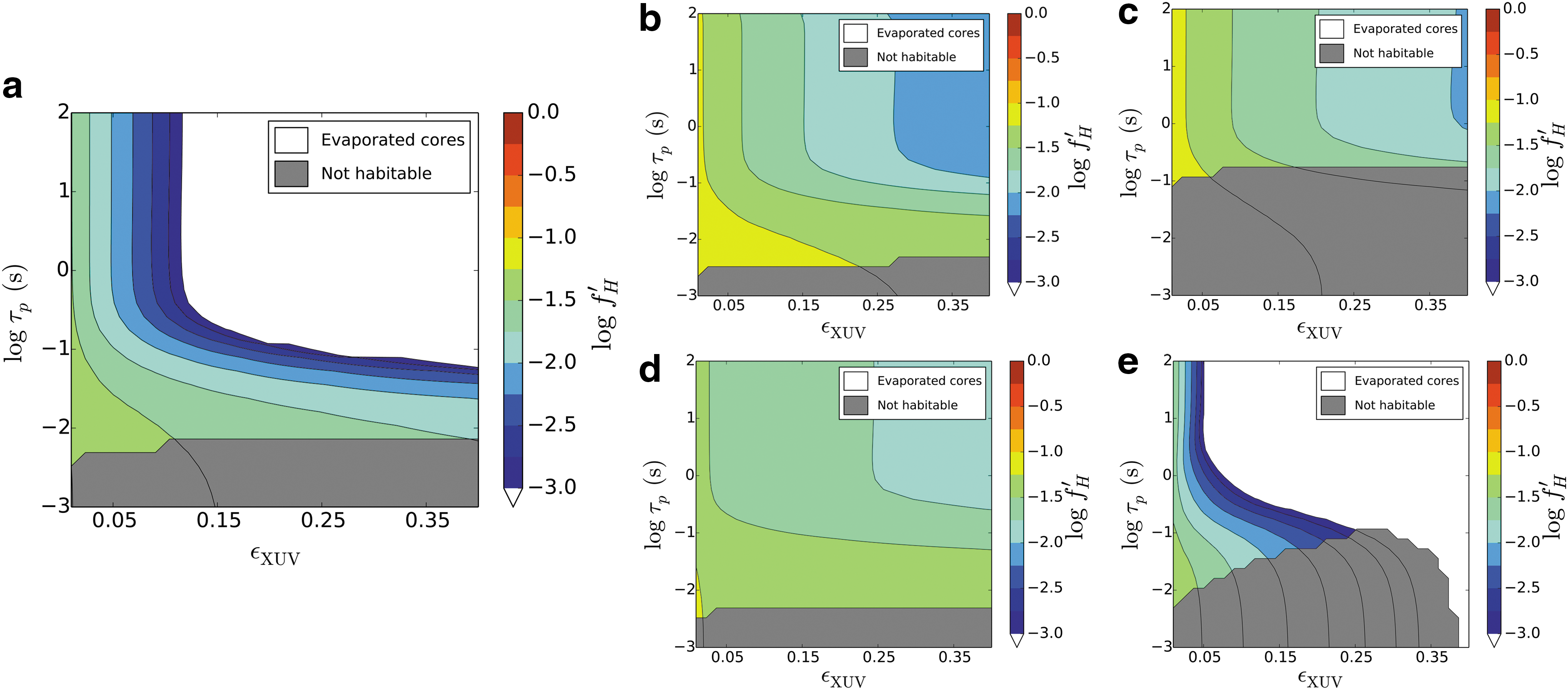
Contours of the log of the hydrogen mass fraction f′
H at 5 Gyr as a function of the tidal time lag τ
p and the XUV absorption efficiency ε
XUV for five integrations of our code. White regions correspond to planets that completely lost their envelopes; dark gray regions indicate planets that are not in the HZ at 5 Gyr.
In the default run (a), we consider a planet with a core mass of 1 M ⊕ and an envelope mass of 1 M ⊕ (f H=0.5) orbiting at 0.07 AU in a highly eccentric (e=0.8) orbit around a 0.08 M ⊙ star. The mass loss mechanism is radiation/recombination-limited escape at high XUV flux and energy-limited at low XUV flux. At a given value of log τ p, say 0, the final hydrogen fraction is a strong decreasing function of ε XUV, as expected: the higher the evaporation efficiency, the smaller the final envelope. Interestingly, the dependence of f′ H on the tidal time lag can be nearly just as strong. At a given value of ε XUV, say 0.35, f′ H depends strongly on τ, varying from 10−1.5≈3% to 0%—that is, the tidal evolution controls whether or not a HEC forms. This is due to the fact that at large τ p tidal migration is fast, bringing the planet into the HZ while its radius is still inflated and the stellar XUV luminosity is higher. Planets with lower values of τ p migrate in later and undergo slower mass loss. At very low τ p, tidal migration is too weak to bring the planets fully into the HZ. The effect is stronger for higher ε XUV: these are planets whose radii decrease very quickly (due to the fast mass loss), slowing down the rate of tidal evolution and keeping them outside the HZ for longer.
In plot (b), we increase the core mass slightly to 1.5 M ⊕. The effect on the mass loss is significant, and HECs no longer form. At high ε XUV and high τ p, the lowest value of f′ H is about 1%. This reinforces what we argued above: HECs are most likely for the lowest-mass cores.
In plot (c), we instead decrease the eccentricity to 0.7. As in (b), HECs no longer form in these runs due to the decreased strength of the tidal evolution, and again the minimum f′ H is about 1%. Note that this does not mean that HECs are more likely at higher eccentricity in general—this is only the case here because we fix the initial semimajor axis at 0.07 AU. At fixed final semimajor axis (i.e., what we can readily observe in actual systems), planets on initially circular orbits will still lose more mass than planets on initially eccentric orbits (which must have formed farther out).
In plot (d), we decrease the saturation time to t sat=0.1 Gyr, which is typical of early M/late K dwarfs (Jackson et al., 2012). No HECs form, and the final hydrogen fraction is less sensitive to both τ p and ε XUV: in general, mass loss is significantly suppressed.
Finally, in plot (e), we force the escape mechanism to be energy-limited only. Since the escape is now entirely controlled by ε XUV, the dependence on this parameter is naturally much stronger, and complete evaporation occurs in this case for ε XUV≳0.32 at any τ p. Because evaporation occurs more quickly in this case than in the other plots, at any given time the planet radii are smaller, resulting in less efficient migration at a given τ p. More planets therefore do not make it into the HZ. Interestingly, for very large ε XUV (≳0.4), all planets make it into the HZ. This is due to the fact that these planets transition from gaseous (low τ p) to gas-free (high τ p, equal to 64 s in these runs) very early on. Despite their lower radii, they benefit from the stronger tidal dissipation of fully rocky bodies and are able to make it into the HZ after 5 Gyr.
In general, the coupling between tides and mass loss is quite complex. For planets with high initial eccentricities, this coupling can ultimately determine whether or not a HEC will form. We discuss this in more detail in Section 4.4.
4.4. Evaporated cores in the habitable zone
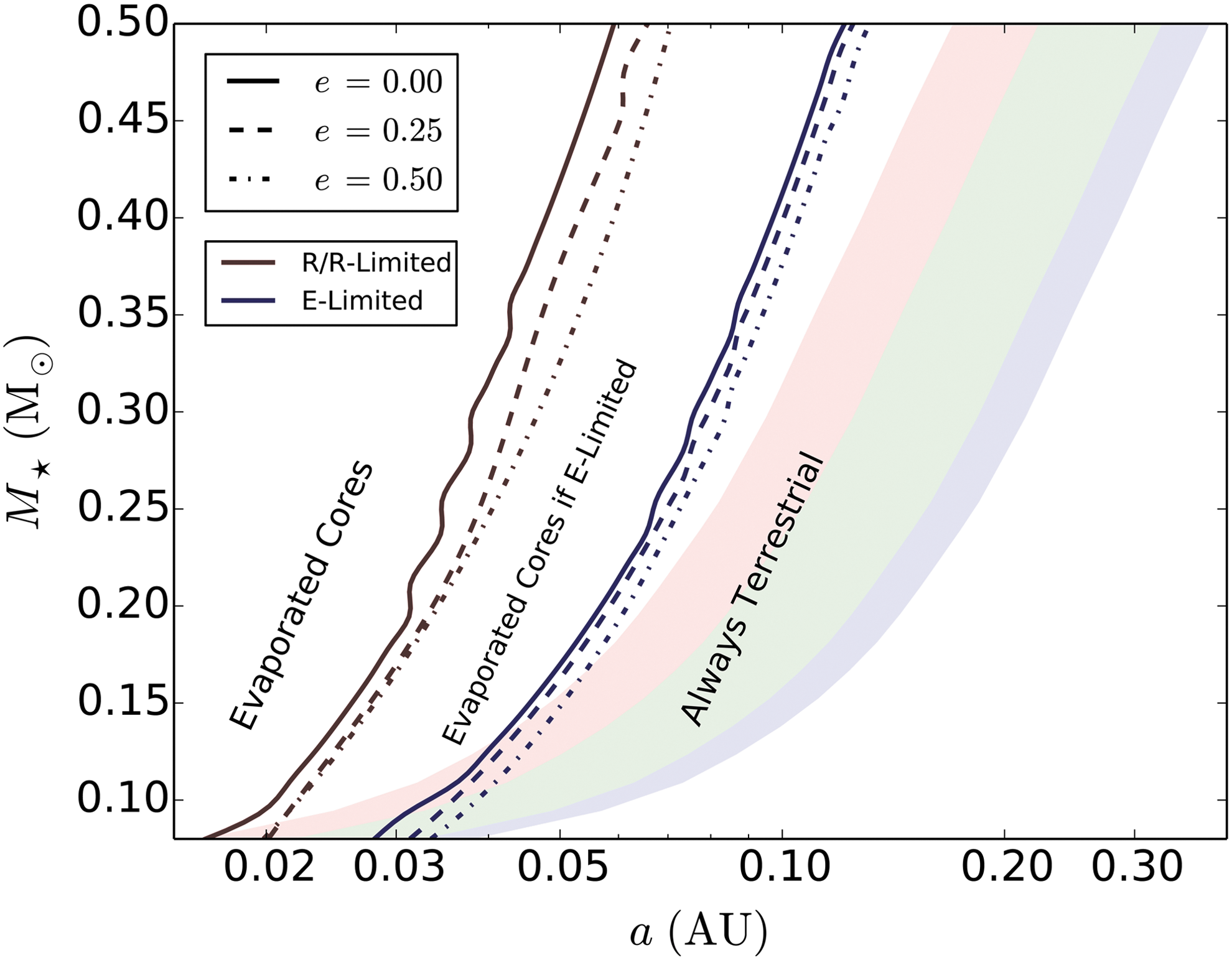
Having shown that HECs are possible in certain cases, we now wish to explore where in the HZ we may expect to find them. For a “terrestrial” (we use this term rather loosely 2 ) planet detected in the HZ, it would be very informative to understand whether or not it may be the evaporated core of a gaseous planet, since its past atmospheric evolution may strongly affect its present ability to host life. To this end, we ran eight grids of 2.7×10⁶ integrations each of our evolution code under different choices of parameters in Table 1. For initial semimajor axes in the range 0.01≤a 0≤0.5, initial eccentricities in the range 0≤e 0≤0.95, and stellar masses between 0.08 M ⊙≤M ★≤0.5 M ⊙, we calculate the final (i.e., at t stop=5 Gyr in the default run) values of a, e, and the envelope mass M H. We then plot contours of M H as a function of the stellar mass and the final semimajor axis and eccentricity (that is, the observable parameters). Since, in principle, the mapping (a 0, e 0, M H 0)→(a, e, M H) is not necessarily a bijection (due to the nonlinear coupling between tides and mass loss and the finite resolution of our grid), the function M H(a, e) may be multivalued at some points. In these cases, we take M H at coordinates (a, e) to be the minimum of the set of all final values of M H that are possible at (a, e). Because of this choice, the M H=0 contour in a versus M ★ plots (Figs. 8 –10) separates currently terrestrial planets that could be the evaporated cores of mini-Neptunes (left) from currently terrestrial planets that have always been terrestrial (right). In other words, we are showing where evaporated cores are ruled out.
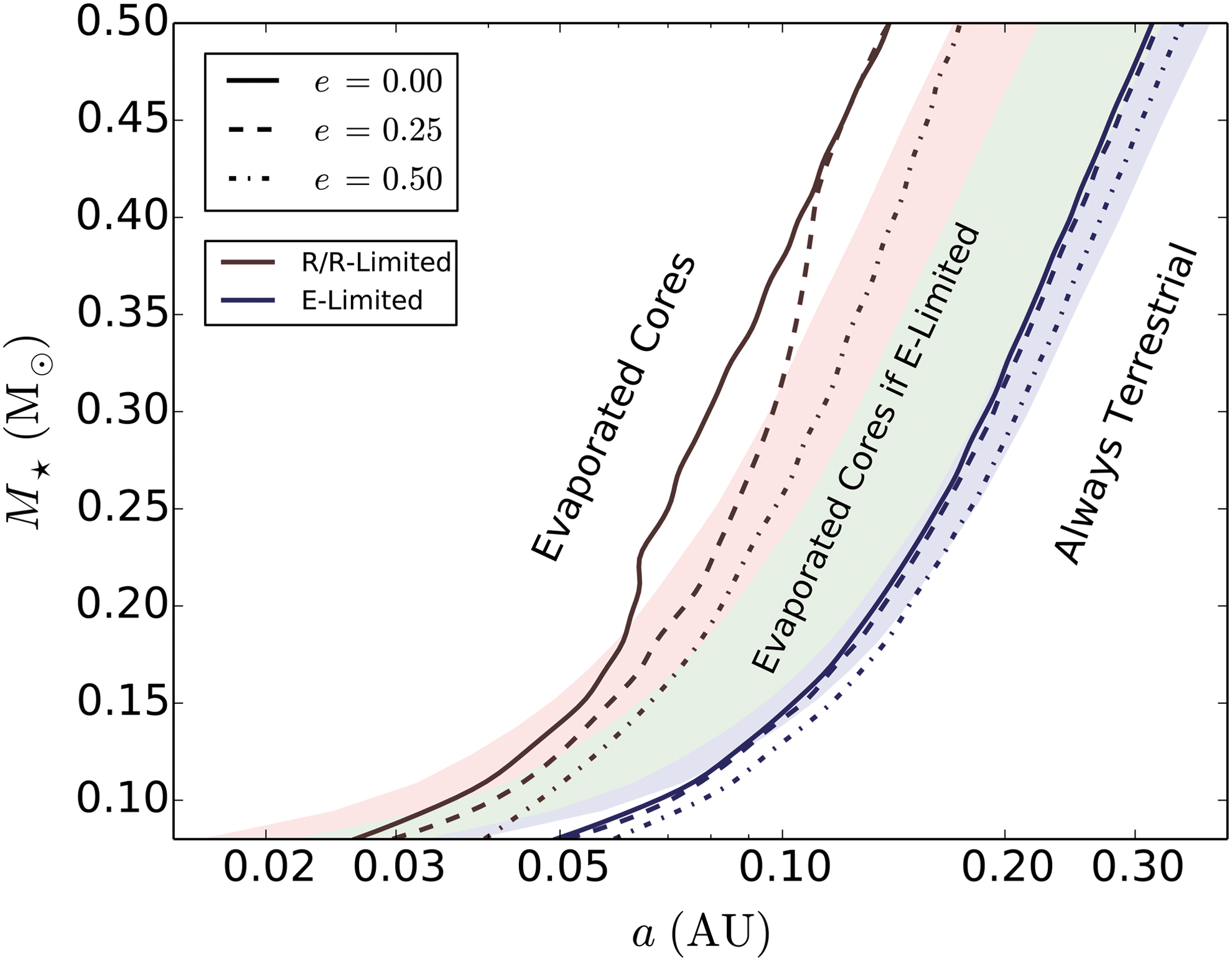
Regions of parameter space that may be populated by HECs, for M c=1 M ⊕, initial M H≤1 M ⊕, and default values for all other parameters. Terrestrial planets detected today occupying the space to the left of each contour line could be the evaporated cores of gaseous planets with f H≤0.5. Planets detected to the right of the contour lines have always been terrestrial/gaseous. Dark red lines correspond to the conservative mass loss scenario, in which mass loss is radiation/recombination-limited at high XUV flux and energy-limited at low XUV flux. Dark blue lines correspond to mass loss via the energy-limited mechanism only. Planets around stars with significant X-ray emission early on are likely to be in the latter regime. Different line styles correspond to different eccentricities today. Terrestrial planets detected at higher eccentricity (dashed and dash-dotted lines) could be evaporated cores at slightly larger orbital separations than planets detected on circular orbits (solid lines). Note that in the energy-limited regime, all 1 M ⊕ terrestrial planets in the HZ of low-mass M dwarfs could be HECs. At higher stellar mass, HECs are restricted to planets in the CHZ and IHZ. In the radiation/recombination-limited regime, the accessible region of parameter space is smaller, but around the lowest-mass M dwarfs HECs are still possible in the CHZ.
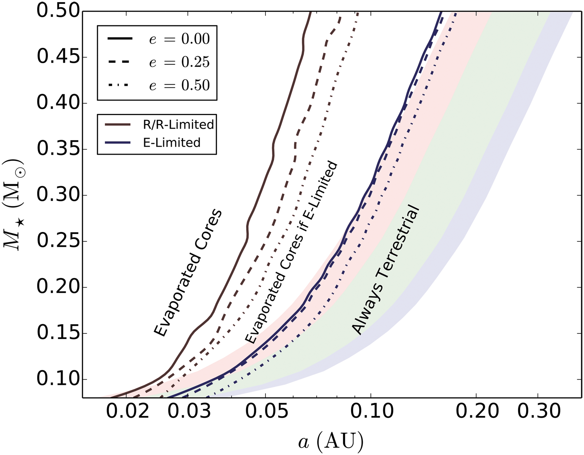
The same plot as Fig. 8 but for a conservative choice of the parameters governing atmospheric escape: a short XUV saturation time t sat=0.1 Gyr and a low XUV absorption efficiency ε XUV=0.15. In this case, HECs are no longer possible for radiation/recombination-limited escape. For energy-limited escape, HECs are only possible in the IHZ of low-mass M dwarfs and in the CHZ of M dwarfs at the hydrogen-burning limit. At high eccentricity (e=0.5), HECs are only marginally more likely.
The same as Fig. 8 but for a higher core mass M c=2 M ⊕. HECs are now confined mostly to the IHZ of low-mass M dwarfs in the energy-limited regime. For planets undergoing radiation/recombination-limited escape, super-Earth HECs may not be possible.
In Fig. 8, we perform the calculations described above for planets with M c=1 M ⊕ and initial f H=0.5 (i.e., initial M H=1 M ⊕). The HZ is plotted in the background for reference, where again the IHZ, CHZ, and OHZ are indicated by the red, green, and blue shading, respectively. Line styles correspond to different final values of the eccentricity (0, solid; 0.25, dashed; and 0.5, dash-dotted). Dark red lines correspond to the M H=0 contours in the radiation/recombination-limited escape model; dark blue lines correspond to the energy-limited model. Note that, though we designate our two models as “energy-limited” and “radiation/recombination-limited,” at low XUV fluxes the escape is energy-limited in both models, since below F crit the energy-limited escape rate is always smaller than the radiation/recombination-limited escape rate. In this sense, the “radiation/recombination-limited model” is always conservative, as the mass loss rate is set to the minimum of Eqs. 5 and 13.
As an example of how to interpret this figure, consider a 1 M ⊕ rocky planet discovered orbiting a 0.2 M ⊙ star at 0.1 AU, that is, squarely within the CHZ. Since this planet lies to the left of all blue curves, under the assumption of energy-limited escape it could be a HEC. On the other hand, if the atmospheric escape were radiation/recombination-limited, this planet must have always been terrestrial.
Next, consider a putative rocky planet discovered around the same 0.2 M ⊙ star skirting the IHZ (i.e., at 0.07 AU). Under the energy-limited assumption, this planet could be a HEC. For radiation/recombination-limited escape, however, whether or not it could be a HEC depends on its present eccentricity. If the planet is currently on a circular orbit, we infer that it has always been terrestrial (since it lies to the right of the e=0 contour). However, since the planet lies to the left of the higher eccentricity contours, if e≳0.25, it could be a HEC.
We conclude from Fig. 8 that, if energy-limited escape is the dominant mechanism around M dwarfs, planets with M p∼1 M ⊕ in the CHZ and IHZ of these stars could be HECs. For M ★≲0.15 M ⊙, HECs may exist throughout the entire HZ. If, on the other hand, these planets are shaped mostly by radiation/recombination-limited escape, HECs are only possible in the IHZ for M ★≲0.2 M ⊙ and in the CHZ of M dwarfs near the hydrogen-burning limit.
The effect of the eccentricity is significant primarily in the radiation/recombination-limited regime, where a lower mass loss rate keeps the planet's radius large for longer than in the energy-limited regime, allowing it to migrate into the HZ faster, thereby enhancing the mass loss rate. In some cases, particularly near the IHZ, the present-day eccentricity yields important information about a planet's evolutionary history: depending on the precise value of e, a given terrestrial planet may or may not be a HEC. However, we urge caution in interpreting the results in Fig. 8 at nonzero eccentricity, given the large uncertainty in the tidal parameters of exoplanets.
On this note, it is important to bear in mind that the curves in Fig. 8 are a function of our choice of parameters in Table 1. To assess the impact of our choice of “default” parameters on these contours, in Fig. 9 we repeat the calculation for more conservative values of the two parameters that govern the mass loss mechanism: the XUV saturation time t sat and the absorption efficiency ε XUV. In this figure, we choose t sat=0.1 Gyr, the nominal value for earlier K/G dwarf stars (Section 2.1), and ε XUV=0.15.
In this grid, all curves shift quite dramatically to lower a, and HECs are no longer possible under radiation/recombination-limited escape. For energy-limited escape, HECs are confined to the IHZ for M ★≲0.15 M ⊙ and the CHZ for M ★≲0.1 M ⊙ at all eccentricities considered here.
Given the large difference between the results of Figs. 8 and 9, care must be taken in assessing whether a planet may be a HEC. Since it is likely that the XUV saturation time is much longer for M dwarfs than for K and G dwarfs, and since our goal at this point is to separate regions of parameter space where HECs can and cannot exist, Fig. 8 is probably the more relevant of the two. We discuss this point further in Section 5.
In Fig. 10, we raise the core mass to M c=2 M ⊕. HECs are now possible only in the IHZ and only in the energy-limited regime. At the lowest M ★, HECs may be possible in the CHZ (energy-limited) and at the very inner edge of the HZ (radiation/recombination-limited). At higher eccentricity, the parameter space accessible to HECs is slightly higher in the energy-limited regime, but it is still a small effect overall. For a conservative choice of escape parameters (t sat=0.1 Myr and ε XUV=0.15) with M c=2 M ⊕, no HECs form anywhere in the HZ.
5. Discussion
5.1. Initial conditions
We have shown that HECs can form from small mini-Neptunes (M p≲2 M ⊕) with H/He mass fractions as high as f H=0.5 around mid to late M dwarfs. However, instrumental to our conclusions is the assumption that these planets formed beyond the snow line and migrated quickly into the HZ at t=t 0. Planets that form in situ in the HZ are unlikely to accumulate substantial H/He envelopes due to large disk temperatures and relatively long formation timescales. Significant gas accretion can only occur prior to the dissipation of the gas disk, which occurs on a timescale of a few to ∼10 Myr; in particular, Lammer et al. (2014) showed that a 1 M ⊕ terrestrial planet generally accretes less than ∼3% of its mass in H/He in the HZ of a solar-type star. Moreover, planets that form in situ do not undergo RLO, since accretion of any gas that would lead to R p>R Roche simply will not take place.
But can mini-Neptunes easily migrate into the HZ? The large number of recently discovered hot Neptunes and hot super-Earths (e.g., Howard et al., 2012) suggests that inward disk-driven migration is a ubiquitous process in planetary systems, as it is highly unlikely that these systems formed in situ (Raymond and Cossou, 2014). Moreover, systems such as GJ 180, GJ 422, and GJ 667C each have at least one super-Earth/mini-Neptune in the HZ (Anglada-Escudé et al., 2013; Tuomi et al., 2014), some or all of which may have migrated to their current orbits. On the theoretical front, N-body simulations by Ogihara and Ida (2009) show that migration of protoplanets into the HZ of M dwarfs is efficient due to the proximity of the ice line and the fact that the inner edge of the disk lies close to the HZ. Mini-Neptunes that assemble early beyond the snow line could in principle also migrate into the HZ, but the migration probability and the distribution of these planets throughout the HZ needs to be investigated further in order to constrain the likelihood of formation of HECs.
A second issue is whether or not Earth-mass cores can accrete large H/He envelopes in the first place. One of our key results is that Earth-mass HECs can form from mini-Neptunes with initial envelope mass fractions of up to 50%; this would require a 1 M ⊕ planetary embryo to accrete an equivalent amount of gas from the disk. While such a planet would be stable against RLO beyond the snow line, whether or not it could have formed is unclear. Gas accretion takes place in two different regimes: (i) a slow accretion regime, in which the envelope remains in hydrostatic equilibrium and gains mass only as it cools and contracts, evacuating a region that is then filled by nebular gas; and (ii) a runaway accretion regime, in which the rapidly increasing mass of the envelope leads to an increase in the size of the Hill sphere and increasingly faster gas accretion (e.g., Pollack et al., 1996). Since the critical core mass for runaway accretion is thought to be somewhere in the vicinity of 10–20 M ⊕ (Pollack et al., 1996; Rafikov, 2006), the progenitors of HECs must accrete their gas slowly. As we mentioned above, Lammer et al. (2014) found that Earth-mass planets typically form with f H≲0.03 in the HZ of solar-type stars. This is consistent with recent analyses of Kepler planet data by Rogers (2014) and Wolfgang and Lopez (2014), who found that most planets with radii less than about 1.5 R ⊕ (corresponding to masses less than ∼5 M ⊕) are rocky, with typical H/He mass fractions of about 1%.
Formation beyond the snow line can increase f H: Rogers et al. (2011) showed that a planet with core mass 2.65 M ⊕ accretes only 0.54 M ⊕ of gas (corresponding to f H≈17%). Bodenheimer and Lissauer (2014), on the other hand, showed that planets with cores in the range 2.2–2.5 M ⊕ generally accrete less than 10% of their mass in H/He. However, these authors terminated gas accretion at 2 Myr. For a longer disk lifetime of 4 Myr, Bodenheimer and Lissauer (2014) showed that a planet with core and envelope masses of 2.8 M ⊕ and ∼1.2 M ⊕, respectively, can form (f H≈30%). This is particularly relevant to planet formation around M dwarfs, as these stars may have disk lifetimes in excess of 5 Myr (Carpenter et al., 2006; Pascucci et al., 2009), which could allow for larger initial H/He envelope fractions.
Nevertheless, while a 1 M ⊕ core with a 1 M ⊕ envelope is probably an unlikely initial condition, it is important to keep in mind that our results apply to planets that form with smaller H/He fractions as well. Figures 8 –10 show where planets with up to 50% H/He can form HECs; planets with lower H/He mass fractions also form HECs at the same values of a and M ★. See Section 5.6 for a more detailed discussion.
5.2. Are HECs habitable?
Under the core accretion mechanism, mini-Neptunes are likely to form close to, or beyond, the snow line, where disk densities are higher due to the condensation of various types of ices; these planets should therefore have large quantities of volatiles, including water, ammonia, and CO2 ices. If we assume a disk composition similar to that around the young Sun, the bulk composition of their cores would probably be similar to that of comets: roughly equal parts ice and silicate rock, similar to what studies predict for the composition of water worlds (Léger et al., 2004; Selsis et al., 2007). Once these planets have migrated into the HZ and lost their envelopes, it is quite likely that they would be water worlds and therefore not “terrestrial” in the strictest sense of the word. Whether or not such planets are habitable may depend on their ability to sustain active geochemical cycles, which are crucial for life on Earth today.
One concern is a possible interruption of the carbon cycle by a high-pressure ice layer at the bottom of the ocean (Léger et al., 2004). Recently, Alibert (2014) calculated the critical ocean mass for high-pressure ice formation, finding that it lies between 0.02 and 0.03 M ⊕ for an Earth-mass planet. If HECs are, in fact, cometlike in composition, a deep ice layer would separate their oceans from their mantles, which could inhibit the recycling of carbon and other bioessential elements between the two reservoirs, a process that is critical to life on Earth. However, whether this is the case is far from settled, as processes involving solid state ice convection could mediate the cycling of these elements. In particular, Levi et al. (2013) and Kaltenegger et al. (2013) presented a mechanism that could recycle CH4 and CO2 between the interior and the atmosphere of water worlds, invoking the ability of these molecules to form clathrates that could be convectively transported through the ice to the surface. Other mechanisms could also exist, and without further modeling, it is unclear whether a high-pressure ice layer poses a threat to habitability.
The probable difference in composition between HECs and Earth is likely to have other geophysical implications. Hydrogen-rich compounds such as methane and ammonia could make up a non-negligible fraction of a HEC's mass, leading to extremely reducing conditions at the surface. These could also end up in a secondary atmosphere along with large quantities of CO2, which could lead to strong greenhouse heating, although it is likely that most of the CO2 and NH3 would be sequestered in the ice mantle (Léger et al., 2004). The compositional difference of HECs would also likely lead to mantle convection and tectonic activity different from Earth's, as well as differences in magnetic field generation by a possible core dynamo. Since both an active tectonic cycle and a magnetic field may be necessary for habitability, these issues need to be investigated further.
Also critical to the habitability of a HEC is its ability to outgas a secondary atmosphere once its primordial envelope is lost. In particular, the secondary atmosphere must be stable against erosion. While the power-law decay in XUV emission after t sat could allow for such an atmosphere to form, low-mass M dwarfs may remain active for t >>1 Gyr. Strong planetary magnetic fields could potentially shield these atmospheres; Segura et al. (2010) showed that flares on the extremely active M dwarf AD Leo would have a small effect on the atmosphere of an Earth-like planet in the HZ provided it has an Earth-like magnetic field. However, interactions with the stellar wind could still pose serious problems to these and other planets in the HZs of M dwarfs. In particular, the high XUV/EUV fluxes of active M dwarfs can lead to significant expansion of the upper atmosphere, potentially causing the radius of the exobase to exceed the distance to the stellar magnetopause (Lichtenegger et al., 2010; Lammer et al., 2011). For a pure N2 atmosphere, Lichtenegger et al. (2010) showed that nitrogen ionized by EUV radiation above the exobase is subject to ion pickup by the solar wind, leading to the complete erosion of a 1 bar atmosphere in as short a time as 10 Myr. A stronger planetary magnetic field or large quantities of a heavier background gas such as CO2 may be necessary to suppress ion pickup and preserve secondary atmospheres on HECs.
Given the complex processes governing the habitability of HECs, a detailed investigation of these issues is left to future work. As we discuss below, stronger constraints on the details of the X-ray/EUV evolution of M dwarfs of all masses are essential to understanding the fate and ultimately the habitability of planets around these stars.
5.3. The need for better constraints
Figure 8 shows that the formation of HECs depends strongly on the atmospheric escape mechanism. As we mentioned earlier, whether a flow is closer to radiation/recombination-limited or energy-limited will depend on the ratio of the X-ray to EUV luminosity of the parent star. Low-mass M dwarfs may have XUV luminosities as high as ∼4×1029 erg/s early on (Section 2.1). If X-rays contribute more than a few percent of this luminosity, low-mass low-density planets in the HZs of these stars may undergo energy-limited X-ray-driven escape (Fig. 11 in Owen and Jackson, 2012). Unfortunately, knowledge of the exact age-luminosity relation in the X-ray and EUV bands for M dwarfs is still very poor, in great part because of the large uncertainties on these stars' ages. However, recent studies suggest that X-rays contribute a significant fraction of this luminosity (for a review, see Scalo et al., 2007). In particular, Stelzer et al. (2013) reported high (L X≳1029 erg/s) X-ray luminosities for a sample of early active M dwarfs in the solar neighborhood, with a steeper age dependence than in far ultraviolet and near ultraviolet bands, which dominate the emission for t≳1 Gyr. This is consistent with Owen and Jackson (2012), who argued that close-in mini-Neptunes may undergo a transition from X-ray-driven escape at early times to EUV-driven escape at later times.
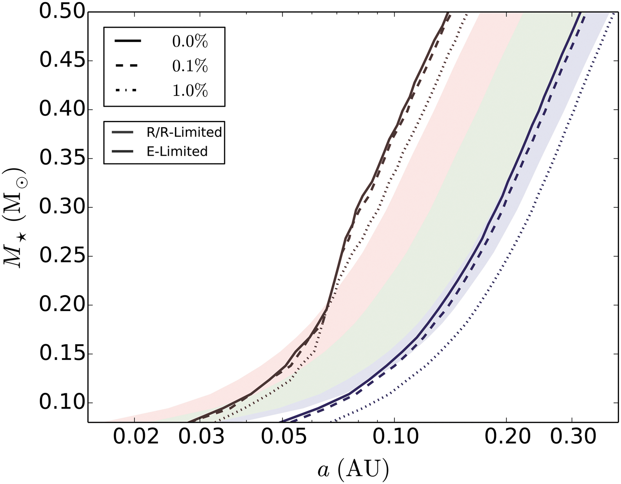
Similar to Fig. 8, but here contours correspond to different choices of final f H (which we denote f′H) for a 1 M ⊕ core on a circular orbit. The solid lines correspond to f′ H=0 and are the same as the e=0 contours in Fig. 8. Dashed lines correspond to the transition between planets that have less than (left) and more than (right) 0.1% H/He (f′ H=0.001) at 5 Gyr. Dotted lines correspond to the 1% H/He (f′ H=0.01) transition. While the f′ H=0.001 contours are barely distinguishable from the f′ H=0 contours, at final f′ H=0.01 the HEC parameter space is significantly larger. However, it is unclear whether planets with f′ H=0.01 could be habitable.
Moreover, atmospheric X-ray heating and cooling is primarily done by metals. As Owen and Jackson (2012) pointed out, atmospheric composition is also likely to play a role in determining whether hydrodynamic flows are EUV- or X-ray-driven. Additionally, the presence of dust in the envelopes of these planets could greatly affect their ability to cool via Lyman α radiation. Absorption of recombination radiation by dust particles lifted high into the envelope by vigorous convection could convert a significant fraction of this energy into heating, which could effectively increase the absorption efficiency ε XUV and bring the flow closer to the energy-limited regime. Unfortunately, our present parametric escape model is unable to address the effect of dust and metal abundances on the escape rate—this issue needs to be revisited in the future with more sophisticated hydrodynamic models.
The difference between Fig. 8 and Fig. 9 is just as significant. At lower t sat and ε XUV, the HEC parameter space is greatly reduced. As we discuss in Section 2.1, the lower value t sat=0.1 Gyr is more representative of K and G dwarfs, while M dwarfs may remain saturated for t sat>1 Gyr. In fact, the energy-limited contours in Fig. 8 closely trace the CHZ/OHZ boundary as M ★ increases, predicting that HECs may even be possible around solar-type stars (not shown). This is of course not the case, since solar-type stars are known to leave the saturation phase around t sat=0.1 Gyr (Ribas et al., 2005). Above a certain value of the stellar mass near the M/K dwarf transition (0.5 M ⊙≲M ★≲0.7 M ⊙), Fig. 9 becomes a better description for HECs; but for low-mass M dwarfs, Fig. 8 is probably more appropriate.
Naturally, the exact value of ε XUV will also affect the possible distribution of HECs within the HZ. Recently, Shematovich et al. (2014) performed numerical simulations to solve the kinetic Boltzmann equation for XUV-irradiated hydrogen atmospheres, finding an upper limit to the heating efficiency of ε XUV≈0.20. Our nominal value ε XUV=0.3 may therefore be an overestimate for many mini-Neptunes. However, given that our goal in this study is to explore where in the HZ HECs are possible and to map regions where the transition from gaseous to terrestrial is not possible, our present approach should suffice. Nevertheless, further studies constraining ε XUV are crucial to improving our understanding of this parameter space.
5.4. Eccentricity effects
From Figs. 8
–10 we see that as we consider planets with higher current eccentricity, the region where evaporated cores are possible overlaps increasingly more of the HZ, particularly in the radiation/recombination-limited regime. This does not necessarily mean that HECs are more likely at high eccentricity—but rather that planets in circular orbits at certain a cannot be HECs, while planets at higher eccentricity can. However, that being said, there is an interesting negative feedback between tides and mass loss that may enhance the probability of HECs on eccentric orbits. A planet with initially high eccentricity will undergo fast tidal evolution (due to the strong β dependence in Eq. 74), particularly if its radius is large (since de/dt∝
We note that Figs. 8 –10 show eccentricity contours only up to e=0.5. At final eccentricities higher than 0.5 today, the contour lines should move farther to the right, increasing the parameter space populated by HECs. However, since high eccentricities today in general require extremely high eccentricities in the past, we do not calculate contours above this level. We note, finally, that even though we run simulations with e 0 as high as 0.95, Figs. 8 –10 remain unchanged for a lower cutoff e 0≲0.7.
5.5. Orbital effects due to Roche lobe overflow
In the present work, we neglect any orbital effects due to RLO, which could in some cases lead to significant outward migration of the planet; see (22). We argued in Section 3.3 that since RLO should occur during the initial stage of migration (i.e., from beyond the snow line into the HZ), modeling it was outside the scope of our study. However, a careful investigation of this initial migration process could uncover interesting couplings. For instance, mini-Neptunes that initially overshoot the HZ would experience strong RLO, which could in principle cause them to migrate back into the HZ. These planets could have lost significantly more mass than the ones we considered here, since both RLO and XUV-driven escape would be stronger in their closer-in orbits.
A second important point concerning RLO-induced migration is that for nonzero eccentricity (22) does not apply. In this case, it can be shown that angular momentum exchange between the gas and the planet at pericenter (where overflow is strongest) leads to a net increase in the eccentricity. In the limiting case that both bodies may be treated as point masses and the mass transfer rate may be approximated as a delta function at pericenter (which is appropriate for high e), Sepinsky et al. (2009) showed that
predicting that both a and e will tend to increase with time (recall that
In other words, at intermediate values of e, the fractional rates of change in the semimajor axis and the eccentricity are comparable, and the eccentricity will increase proportionally to the semimajor axis.
As e increases, so does the atmospheric mass loss rate (via K ecc), the RLO rate (modulo the increase in a), and the rate of tidal evolution, leading to potentially faster mass loss and rich couplings between these different processes. We will consider all these effects in a future paper.
5.6. Different f H
Figures 8 –10 correspond to planets with initial hydrogen fraction f H=0.5. Planets with lower initial f H are naturally more unstable to complete loss of their envelopes—this would move all contours to the right, expanding the region where HECs are possible. However, for a different choice of initial f H in the range 0.1≲f H≲0.5, the figures change very little: at constant core mass, it is only marginally harder to fully evaporate a f H=0.5 envelope than it is to evaporate a f H=0.1 envelope (see discussion below). This is due to both RLO, which dramatically reduces the envelope mass early on, and the fast atmospheric escape for extremely inflated planets. In Fig. 5a, for instance, the envelope fraction decreases by a factor of 10 within the first ∼10 Myr due to energy-limited escape. The escape process is in general very fast for large f H and bottlenecks for f H≲0.1; thus the HEC boundary is relatively insensitive to the exact choice of the initial f H.
Along the same lines, we can ask how the choice of final f H (which here we denote f′H) affects our results. In this study, we define an evaporated core as a planet with f′ H=0 and no atmosphere. However, mini-Neptunes with substantial gaseous envelopes that evaporate down to f′ H∼0.01 become fundamentally solid planets. At such low f′ H, additional nonthermal mass loss processes, including flaring events and interactions with the stellar wind, may significantly erode the remaining envelope. Investigating the habitability of planets with nonzero f′ H is beyond the scope of this paper, but it is worthwhile to consider how an alternative definition of a “habitable evaporated core” affects our results. To this end, in Fig. 11 we plot contour lines corresponding to three different choices of the critical f′ H below which we consider a planet to be a HEC. Solid lines correspond to f′ H=0 (the default choice); dashed lines correspond to f′ H=0.001; dotted lines correspond to f′ H=0.01. Note that in the radiation/recombination-limited regime, this choice does not significantly affect evaporated cores in the HZ. However, for f′ H=0.01, all planets undergoing energy-limited escape in the HZ could be HECs.
Earths and super-Earths with up to a few percent of their mass in H/He may still harbor liquid water oceans, so at this point their habitability cannot be ruled out. At higher f′ H, however, the surface pressures in excess of ∼1 GPa (e.g., Choukroun and Grasset, 2007) result in the formation of high-pressure ices, at which point the planet will likely no longer be habitable.
5.7. Other atmospheric escape mechanisms
We modeled the XUV emission of M dwarfs as a smooth power law, but active M dwarfs are seldom so well behaved. Frequent flares and coronal mass ejections punctuate the background XUV emission and will lead to erosion of planetary atmospheres beyond what we model here. During flares, the ratio of the X-ray to bolometric luminosity (L X/L bol) can increase by up to 2 orders of magnitude (Scalo et al., 2007). Moreover, interactions with the stellar wind and nonthermal escape mechanisms such as ion pickup and charge exchange can lead to a few Earth-ocean equivalents of hydrogen from these planets (Kislyakova et al., 2013, 2014). However, as Kislyakova et al. (2013) demonstrated, the escape rate due to these processes generally amounts to only a few percent of the hydrodynamic escape rate. Including these nonthermal mechanisms would thus have a minor effect on our results.
In this study, we also neglect the effects of magnetic fields. The presence of a strong planetary magnetic field may inhibit escape during flares and possibly decelerate the mass loss rate if the planetary wind is ionized. Since a strong magnetic field is likely a requirement of surface habitability around an M dwarf (Scalo et al., 2007), this point must be addressed in future work.
Finally, stars less massive than about 0.1 M ⊙ may be in a “supersaturation” regime early on, saturating at XUV fluxes 1 or even 2 orders of magnitude below higher-mass M dwarfs (Cook et al., 2014). This could reduce escape rates from planets around M dwarfs close to the hydrogen burning limit.
5.8. Multiplanet systems
In this paper, we restricted our calculations to single-planet systems. However, many of the super-Earths and mini-Neptunes recently detected by Kepler reside in multiplanet systems, such as Kepler-32 (Fabrycky et al., 2012), Kepler-62 (Borucki et al., 2013), and Kepler-186 (Quintana et al., 2014). Moreover, Swift et al. (2013) demonstrated how the five-planet system Kepler-32 could be representative of the entire ensemble of Kepler M dwarf systems, arguing that multiplicity could be the rule rather than the exception for these stars.
While tidal processes still operate in systems with multiple planets, the orbital evolution of individual planets will be much more complex. In general, though tidal dissipation may still lead to a decrease in the semimajor axis, the eccentricity evolution will be governed by secular interactions between the planets. The coupling between mass loss and tidal evolution we investigated in Section 4.3 would likely be weaker, particularly for closely packed coplanar systems where the eccentricities are necessarily low. However, planet-planet interactions could allow for even richer couplings to the atmospheric evolution of planets in the HZ.
Consider, for instance, the case of a terrestrial planet in the HZ and a mini-Neptune interior to the HZ. Both mass loss and tidal dissipation scale inversely with the semimajor axis, so both effects could strongly shape the fate of the inner planet, which could in turn affect both the orbital and atmospheric evolution of the HZ planet in complex ways. The same could happen for a planet overflowing its Roche lobe interior to the HZ, which as we argued in Section 5.5 could experience large changes in a and e.
Similarly, consider a scenario in which a planet in the HZ loses mass at the same time as it is perturbed by a more massive companion exterior to the HZ. As the planet's mass decreases, it will undergo larger swings in eccentricity, which in turn lead to faster mass loss and stronger orbital evolution.
Another interesting scenario involves planets close to mean motion resonances. For a system of two planets in resonance, Lithwick and Wu (2012) and Batygin and Morbidelli (2013) showed that the presence of a dissipative mechanism such as tidal evolution naturally leads to the repulsion of the two planets' orbits: the inner planet's orbit decays, while the outer planet gets pushed outward. In the hypothetical case of two mini-Neptunes in resonant orbits interior to the HZ, this mechanism could result in the migration of the outer planet into the HZ, having lost significantly more mass (due to its initially smaller orbit) than if it had originated exterior to the HZ and migrated inward. A chain of resonant planets, which is a potential outcome of disk-driven migration (Terquem and Papaloizou, 2007; Ogihara and Ida, 2009), could have similarly interesting consequences on planets in the HZ.
All these scenarios, which involve coupling between atmospheric mass loss, tidal evolution, and secular planet-planet interactions, probably occur even for planets outside the HZ. Modeling this coupling could be critical to understanding systems like Kepler-36 (Carter et al., 2012), where two planets with semimajor axes differing by ∼10% have a density ratio close to 8, which Lopez and Fortney (2013) showed could be the result of starkly different mass loss histories. Future work should investigate how mass loss modifies the orbital interactions in multiplanet systems.
5.9. Other caveats
5.9.1. The habitable zone
Yang et al. (2013) argued that cloud feedback on tidally locked planets can greatly increase the planetary albedo and move the IHZ in by a substantial amount. Similarly, Abe et al. (2011) showed that planets with limited surface water are stable against runaway greenhouses at greater insolation than Earth, which also decreases the IHZ distance. Since evaporated cores are more likely at smaller a, a closer-in inner edge to the HZ could greatly increase the parameter space available to these planets. However, as we argued in Section 5.2, HECs are likely to have abundant surface water.
Luger and Barnes (2014) showed that terrestrial planets in the HZ of M dwarfs may experience long runaway greenhouses during their host stars' extended PMS phases, during which time water loss to space can lead to their complete desiccation, rendering them uninhabitable. HECs are naturally more robust against severe water loss, given that their initially dense H/He envelopes can shield the surface and lower atmosphere from XUV radiation. Once the envelope is lost, water loss from the surface could occur, but by that point the stellar XUV flux will be much lower. Future work will address the fate of the water on HECs in detail.
5.9.2. Thermal evolution
As mentioned before, we do not consider how the mass loss rate affects the planet radius, but instead assume the radius instantaneously returns to the “equilibrium” value for the given age, mass, and hydrogen fraction. In reality, the radius is likely to remain inflated for some time, particularly for fast mass loss (Lopez et al., 2012). Because our radii decrease too quickly, the mass loss feedback on the tidal evolution is always negative; mass loss always acts to dampen the tidal evolution. However, accurate modeling of the radius could enable a positive feedback, in which the effect of the decreasing mass (higher da/dt) overpowers the effect of the decreasing radius (lower da/dt) in (60) and (73), leading to faster orbital decay.
Currently, our planet radii are also independent of both the insolation and the degree of tidal heating. Under the extremely high fluxes and strong tidal forces at early times, planets in the HZs of M dwarfs are likely to be significantly more inflated than modeled here, resulting in faster atmospheric mass loss and likely a higher probability of complete envelope loss. We also do not model radiogenic heating, which could further add to the inflation of the planet. In this sense, our results are conservative, and HECs may in fact be possible at larger distances from their parent stars. A self-consistent thermal evolution model must be developed to accurately address this point.
We also emphasize that the quasi-static approximation (see the Appendix) may not be valid for the most inflated planets on eccentric orbits above e≈0.4. Given the large uncertainty concerning the orbital migration due to RLO for planets on eccentric orbits, we urge caution in interpreting our results quantitatively for highly eccentric planets.
5.9.3. Tidal evolution
Given that the CPL tidal model is accurate only to second order in eccentricity, most of our integrations were performed under the CTL framework. At low e, however, these models predict qualitatively similar results for both the orbital migration and the coupling to the mass loss processes. At high e, on the other hand, tidal models lack observational validation, given the relatively low eccentricities of the major bodies in our solar system. We again urge caution in interpreting quantitative results for e≳0.5.
Recall that our values of Q
p and τ
p are fixed throughout the integrations and change discontinuously to the more dissipative rocky values as soon as the envelope is lost; this is certainly an oversimplification. Though we defined Q via its relationship to the phase lag in (19), it may also be defined as the specific dissipation function (Goldreich and Soter, 1966), defined as
where E 0 is the maximum tidal energy stored in the system, and the integral is the energy dissipated per cycle. Q is therefore inversely proportional to the dissipation per unit energy stored. Planets with large values of f H, where the dissipation throughout most of the body is small, should therefore have large values of Q p; rocky planets with small f H, conversely, have large specific dissipation rates and correspondingly low values of Q p, in agreement with the remarks in Section 2.4.1. Therefore, we would expect that as planets lose mass, Q p should decrease, corresponding to an increase in τ p. Modeling Q p(f H) and τ p(f H), however, is outside the scope of this paper and will be considered in future work. We simply note that, as planets lose mass, the decreasing value of Q p/increasing value of τ p should offset the decreasing radii, leading to stronger tidal evolution and stronger couplings than reported here.
One must likewise be careful in choosing the planet radius that goes into calculating the tidal evolution. This radius should be the effective radius of the dissipating material and is thus dependent on the chosen value of Q p and τ p; for high Q p/low τ p, the radius should probably be that of the envelope. We took this to be R p, the 20 mbar radius shown in the tracks in Fig. 3; other choices of the tidal radius will lead to different evolutions.
We only consider planets with zero initial obliquity. For nonzero obliquity, the tidal evolution equations must be modified and will lead to differences in the evolution; see the works of Heller et al. (2011) and Barnes et al. (2013). We also ignore the spin-up of the planet as it thermally contracts over time, since it should return to the equilibrium spin almost instantaneously. The excess angular momentum would most likely be absorbed into the orbit, but it is a small enough fraction of the orbital angular momentum that it can be safely neglected.
Finally, we note that throughout this paper we set t stop=5 Gyr, based on the age of the Solar System. For systems older than 5 Gyr, our results should change little, since both the tidal and atmospheric evolution will have strongly tapered off by this time. Younger systems, however, may still be in the throes of tidal decay and mass loss processes, and this must be kept in mind when searching for HECs.
6. Conclusions
We have shown that gas-rich mini-Neptunes that migrate early (t ≲ 10 Myr) into the HZs of M dwarfs can naturally shed their gaseous envelopes and form gas-free Earth-mass planets. Together, RLO and hydrodynamic escape can remove up to a few Earth masses of hydrogen and helium from these planets, potentially turning them into “habitable evaporated cores” (HECs). This process is most likely for mini-Neptunes with solid cores on the order of 1 M ⊕ and up to about 50% H/He by mass, and can occur around all M dwarfs, particularly close to the IHZ. HECs are less likely to form around K and G dwarfs because of these stars' shorter superluminous PMS phases and shorter XUV saturation timescales. Furthermore, we find that HECs cannot form from mini-Neptunes with core masses greater than about 2 M ⊕ and more than a few percent H/He by mass; thus, massive terrestrial super-Earths currently in the HZs of M dwarfs have probably always been terrestrial. Our results are thus similar to those of Lammer et al. (2014), who showed that planets more massive than ∼1.5 M ⊕ typically cannot lose their accreted nebular gas in the HZs of solar-type stars.
Whether or not a given mini-Neptune forms a HEC is highly dependent on the early XUV evolution of the host star. In particular, a long XUV saturation timescale (t sat≳1 Gyr) is needed to fully evaporate the envelopes of mini-Neptunes in the HZs of early and mid M dwarfs. While a large t sat is consistent with the long activity timescales (West et al., 2008) and long spin-down times (Pizzolato et al., 2000) of M dwarfs, more observations are needed to pin down t sat for these stars. Moreover, the relative strength of the X-ray and EUV luminosity early on also affects whether or not HECs can form, as this determines whether the atmospheric escape is energy-limited or radiation/recombination-limited. In the energy-limited regime, which occurs for an X-ray-dominated flow, the escape is fast, and HECs can form throughout most of the HZs of all M dwarfs. In the radiation/recombination-limited regime, which applies to an EUV-dominated flow, HECs only form close to the inner edge of low-mass M dwarfs.
We further find that HECs can form from planets on circular as well as eccentric orbits, though they are marginally more likely to have higher e in the long run. While there exist feedbacks between atmospheric mass loss and tidal evolution, we find that these are only significant at e≳0.5; in these cases, whether or not a HEC forms can depend just as strongly on the tidal properties of the planet as on the efficiency of the atmospheric escape.
Many of the Earth-mass terrestrial planets detected in the HZs of M dwarfs in the coming years could be HECs. These planets should have abundant surface water and are likely to be water worlds, whose potential for habitability should be investigated further.
Footnotes
Abbreviations
Acknowledgments
We wish to thank Russell Deitrick, Eric Agol, and the rest of the VPL team for their insightful suggestions and many rich discussions. We also wish to thank two anonymous referees for their excellent comments and suggestions. This work was supported by the NASA Astrobiology Institute's Virtual Planet Laboratory under Cooperative Agreement solicitation NNA13AA93A and by a generous fellowship from the ARCS Seattle chapter.