Computational Fluid Dynamics Simulations to Assess Spatial Variability and Optimal Ventilation Scenarios for Biological Laboratory Exposures

Abstract

Introduction:

A significant amount of uncertainty exists regarding potential human exposure to laboratory biomaterials and organisms in Biosafety Level 2 (BSL-2) research laboratories. Computational fluid dynamics (CFD) modeling is proposed as a way to better understand potential impacts of different combinations of biomaterials, laboratory manipulations, and exposure routes on risks to laboratory workers.

Methods:

In this study, we use CFD models to simulate airborne concentrations of contaminants in an actual BSL-2 laboratory under different configurations.

Results:

Results show that ventilation configuration, sampling location, and contaminant source location can significantly impact airborne concentrations and exposures. Depending on the source location and airflow patterns, the transient and time-integrated concentrations varied by several orders of magnitude. Contaminant plumes from sources located near a return vent (or exhaust like a fume hood or ventilated biosafety cabinet) are likely to be more contained than sources that are further from the exhaust. Having a direct flow between the source and the exhaust (through-flow condition) may reduce potential exposures to individuals outside the air flow path.

Conclusion:

Designing a BSL-2 room with ventilation and airflow patterns that maximize through-flow conditions to the return/exhaust vents and minimize dispersion and mixing throughout the room is, therefore, recommended. CFD simulations can also be used to assist in characterizing the impacts of supply and return vent locations, room layout, and source locations on spatial and temporal contaminant concentrations. In addition, proper placement of particle sensors can also be informed by CFD simulations to provide additional characterization and monitoring of potential exposures in BSL-2 facilities.

Introduction

Despite the explosive growth in biotechnology, the potential for human exposure to laboratory biomaterials and organisms, while conducting laboratory research, is still poorly understood, as are the potential consequences of such exposures. This gap was recently acknowledged in the U.S. Executive Order on Advancing Biotechnology and Biomanufacturing Innovation for a Sustainable, Safe, and Secure American Bioeconomy. ¹ Section 9 focuses on reducing the biosafety and biosecurity risks presented by advances in biotechnology, biomanufacturing, and the bioeconomy.

ABSA International, ² a U.S.-based association for biosafety and biosecurity professionals, maintains a database of reported exposures to biological materials while working in laboratories (laboratory-acquired infections [LAIs]) on its website (my.absa.org/LAI). The development of this database and the criteria utilized to populate it are described by Gillum et al. ³ Although LAI reports could provide the basis for identifying the exposure risks, the data are not comprehensive, as it typically only captures those exposures that result in symptomatic outcomes (e.g., disease diagnosis and treatment) and are reported. It is likely that “silent” exposures—that is, to materials that do not give rise to noticeable symptoms yet may nonetheless pose a health risk—are unaccounted for in this database.

Our analysis of 539 international reports in the database (as of September 2021) indicates that in many reported cases, the cause(s) of the LAI were unknown and/or unattributable to a specific laboratory procedure or set of procedures. We found unattributable LAIs constituted between 26% and 47% of reported LAIs when looking for the past six decades. Before 1960, only 7% of LAIs were unattributable. The overall number of reported LAIs varied across the decades as well, increasing in number until 2000–2009, then decreasing in the past decade. Although it is intriguing to speculate the cause of the rise in unattributable LAIs since 1960, it is difficult to assign the cause of the increase without additional information and further investigation.

We found LAIs attributable to laboratory procedures generally fell into six broad categories: animal work (24%), sample transfer (24%), examination (5.5%), end-of-life sample management (4.5%), sample mixing (4.1%), and changing material state (2.8%). Our review of the literature, reflecting 25 separate publications, we found studies dating back to the 1940s that looked at the potential for laboratory procedures to release biological materials “into the air” as either droplets or droplet nuclei. Most of these studies were conducted in the 1960s with a handful of more recent publications in the early 2000s. ⁴

Studies modeling fluid dynamics also exist during this timeframe but are not specific to laboratory procedures. We focused our review on methods relevant to one of the three defined laboratory procedures: transferring, mixing, or changing material state. All the studies used tracer organisms and a few used chemical surrogates. Most employed air samplers and subsequent testing of the collected samples to define either the concentration or presence of biological material released into the air during the procedure. Following are short summaries of our findings from the literature:

Studies of material transfer considered the potential for aerosol formation caused by opening screwcap bottles^5,6 and defined exposure potential for pipetting, opening of vials both from rest and after the material inside was blended. ⁷ Li et al. ⁸ used a micro-cluster sampling device focusing on pipetting and egg inoculation. Pottage et al. ⁹ focused on exposure potential from serial dilution and plating. Bennett ¹⁰ focused on pipetting, plating, and opening of Eppendorf tubes.

Four reports were found that assessed laboratory exposure potential from the mixing of biological materials by centrifugation, stirring, and vortexing.^6,8,10,11 The only studies on exposure potential from sonication, shaking, or rolling were in the case of an accident or system failure. As we found for material transfer, all the studies used tracer organisms, air samplers, and subsequent testing of the collected samples.

The few studies we identified that focused on changing the state of the materials were based on grinding and bead blasting. No studies were identified considering inactivation, extraction, genetic modification, freezing, drying, aerosolization, or liquefying. All of these have been qualitatively defined as having the potential to create an exposure due to release “into the air,” but specific studies were not found during the literature search. The results of two studies^8,10 highlighted a low but existing potential for release of biological materials “into the air.” Additional studies include the use of autoanalyzers, ⁶ the use of flow cytometry,^12,13 the act of plate sniffing, ¹⁰ use of a microtonometer, ⁶ and laboratory accidents. ¹⁴

Considering the trends in the reported LAI data—specifically that more than a third of reported LAIs do not specify the laboratory procedure(s) associated with the infection—coupled with the reflection that many of the studies of airborne releases of biological materials were conducted decades ago and may not necessarily represent current procedures and equipment in use today, we reflected the utility of more structured airflow modeling was needed, specifically considering procedures that could cause an airborne release. Airflow modeling could help identify the laboratory environmental factors that contribute to the spread (or containment) of biological materials undergoing airborne release and begin to fill in the gaps in understanding between laboratory procedures that have the potential to cause airborne releases and those that result in laboratory worker exposures.

This article presents a pilot study reflecting the use computational fluid dynamics (CFD) modeling in consideration of airborne particle movement within a laboratory. This aligns with recommendations from Kolesnikov ¹⁵ on the utility of CFD tools to better characterize the impact of ventilation, source location, and mixing on exposure risks. This study also complements work by Hwang and Hong ¹⁶ on using CFD in understanding airborne concentrations. The model focuses on the impact of source location, sampling location, and ventilation configuration on contaminant concentrations and potential airborne exposure hazards in a defined Biosafety Level 2 (BSL-2) facility.

Materials and Methods

Sandia's Human Studies Board determined that this study does not constitute human subject research (HSR).

CFD modeling was used to simulate aerosolized releases of biomaterials in a BSL-2 laboratory. The movement of aerosolized materials in the ventilated room was modeled using a tracer gas with the same properties of air. Several modeling and experimental studies have shown that small particles (a few microns or smaller) follow the bulk airflow and can be accurately represented by a tracer gas. ¹⁷ In the experimental study of Bivolarova, ¹⁸ particles of three sizes (0.07, 0.7, and 3.5 μm) and nitrous oxide tracer gas were generated in a room simultaneously at the same location with various ventilation rates and configurations. Sampling at different locations within the room showed that “tracer gas can be used to evaluate the distribution of aerosol particles in ventilated rooms.” Gupta ¹⁹ and Zhang ¹⁷ also concluded that small particles behaved like a tracer gas and followed the bulk airflow during testing and modeling of particle transport in an airplane cabin.

Solidworks Flow Simulation is a commercial software package ²⁰ used to perform the CFD simulations. Flow Simulation solves the conservation of mass, momentum, energy, and species equations using a discrete numerical finite-volume approach. For turbulent flows, Flow Simulation solves the time-averaged Navier–Stokes equations and employs a k-ɛ turbulence model using a laminar/turbulent near-wall model with modified wall functions. ²⁰ Meshing is performed using a combination of hexahedral and polyhedral elements, which accommodate curved boundaries between phases or materials.

Spatial derivatives are approximated with implicit difference operators of second-order accuracy, and time derivatives are approximated with an implicit Euler scheme of first-order accuracy. The time-step size at each iteration is determined using the Courant–Friedrichs–Lewy convergence criterion, where the smallest cell size and a characteristic velocity of the flow field are used. Solidworks Flow Simulation includes solution-adaptive meshing, which splits the mesh cells in the high-gradient flow regions and merges cells in low-gradient regions during the solution.

Refinement was also applied to fluid–solid boundaries in the model domain, and a grid convergence study was performed using multiple mesh resolutions to ensure that the simulated quantities were independent of the selected mesh resolution. Although experiments were not conducted in this study to validate the models, the same modeling approach and tools were used in previous studies by the authors that were validated using airborne pathogen-transport data,^21–23 which gives confidence in the current models. Additional details of the numerical formulations, conservation equations, constitutive relations, meshing, and solution techniques can be found in the technical reference manual. ²⁰ Flow Simulation is integrated within the 3D CAD package Solidworks, which makes geometry and mesh creation seamless and efficient for various scenarios and configurations.

Room Description

A BSL-2 laboratory room was modeled in Solidworks based on a BSL-2 laboratory in Livermore, California. This room was selected as a representative BSL-2 facility due to its size, room configuration, equipment, and ventilation. The room dimensions and ventilation configuration are shown in Figure 1. The room consists of two sets of double doors—a main entrance to the east and a second entrance to the north. The ventilation consists of four ∼2 × 2 feet supply vents (diffusers) and two return vents in the ceiling (see Boundary Conditions section for more details).

Figure 1.

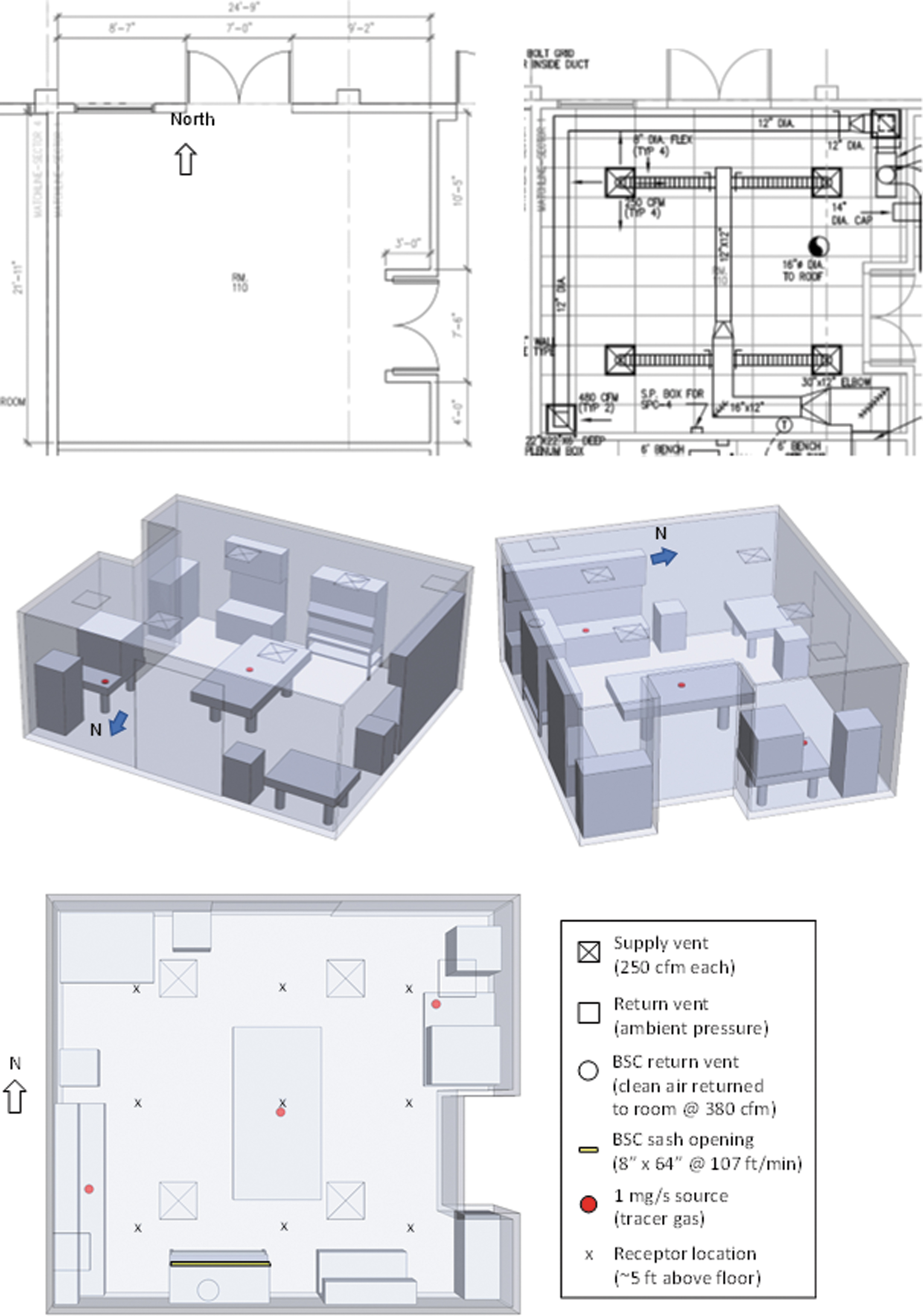
Top: Room dimensions (left) and ventilation (right) for the BSL-2 laboratory. Middle: Two views of the BSL-2 laboratory created in Solidworks. The red disks are aerosol release locations in the CFD modeling. Bottom: Plan view of the BSL-2 laboratory showing boundary conditions used in CFD model. BSL-2, Biosafety Level 2; CFD, computational fluid dynamics.

The room consists of standard laboratory furniture and equipment along the walls, including a biosafety cabinet (BSC) that filters and recirculates air back into the room. A large optical table with materials and equipment sits in the middle of the room. For simplicity, overhead cable trays and smaller equipment, materials, and computer peripherals on the tables and countertops were not modeled in the CFD simulations.

In addition, the room was assumed to be isothermal with adiabatic surfaces and no heat sources. Workers were also not modeled in this study. Although human bodies can cause natural convection due to thermal gradients and obstructions to airflow, ²² the impact of workers on the order-of-magnitude differences in concentrations between the scenarios was not expected to change significantly. The primary objective was to evaluate the relative impact of different contaminant source locations as opposed to characterizing the absolute concentrations and flow behavior, which would require simulation of uncertain transient human motion and behavior that is beyond the scope of this study.

Together with the room layout and dimensions shown in Figure 1, the furniture and major pieces of equipment were measured and modeled in Solidworks. Figure 1 shows two views of the three-dimensional model in Solidworks. Although not exact, the model provides a reasonable representation of the BSL-2 laboratory for the purposes of simulating the impacts of ventilation and room configurations on airborne concentrations and potential exposure risks. Again, the goal was to evaluate the potential relative impacts of different contaminant source locations at different locations within the BSL-2 room and not the absolute concentrations within the room. By maintaining constant geometric and flow-boundary conditions within the simulated room, our goal was to estimate the order-of-magnitude relative impacts among the different scenarios on airborne concentrations.

Boundary Conditions

Figure 1 shows the boundary conditions that were used in the CFD model. Four supply vents introduced 250 cubic feet per minute (cfm) each of clean air into the room, yielding an air exchange rate of ∼10 air changes per hour. The 24″ × 24″ Titus diffusers were modeled with a 45° downward inflow in four directions (N, E, S, and W) corresponding to the four triangular quadrants of each diffuser as shown Figure 1. The air introduced through the diffusers was removed through two 24″ × 24″ return vents located in the NE and SW corners of the room.

The turbulence intensity and length of the airflow boundary condition at the diffusers was assumed to be 2% and 0.03 m, respectively, which was the recommended default values in Solidworks Flow Simulation. Because our goal was to evaluate the relative impacts of the contaminant source locations on order-of-magnitude differences in concentrations within the room, maintaining constant turbulence parameters in each of the scenarios was believed to be sufficient for the purposes of this study. Previous studies have shown that the turbulence intensity can vary “remarkably” with “no generally accepted relationship” in well-ventilated rooms. ²⁴ Therefore, the recommended default values were used in the CFD simulations.

An outlet flow boundary condition was applied to the 8″ × 64″ sash opening of a BSC located along the south wall of the room with an average velocity of 32.6 meter/min. The air was returned to the room through a 14″ circular opening on top of the BSC. The returned air was assumed to be filtered and clean. Steady-state flow simulations were first established in Solidworks Flow Simulation. Once the flow field reached steady state, the flow field was “frozen,” and contaminant releases were introduced into the room for 1 h.

Tracer Gas Releases

Three source locations for contaminant releases were simulated as indicated by the three 6″ red disks shown in Figure 1: the NE corner, the center, and the SW corner of the laboratory. An arbitrary release rate of 1 mg/s of tracer gas with thermophysical properties of air was applied to the top surface of each of the three disks. The mass fraction of the released contaminant in air was assumed to be one for ease of normalization. These contaminant boundary conditions can be thought of as uncovered petri dishes or containers that are perhaps being stirred or sonicated, releasing aerosols at a constant rate continuously into the air. It should be noted that the simulated release rate was small (<1 mL/s or 0.002 cfm) relative to the bulk flow of the ventilation system and did not alter the local airflow pattern near the contaminant source.

Nine sampling/receptor locations were monitored in the simulations at an elevation of ∼5 feet throughout the room as a function of time for 1 h (see “x” receptor locations in Figure 1). The transient and time-integrated concentrations at each location were reported and compared for the different release locations.

Results

Airflow Pattern

The simulated steady-state airflow pattern in the BSL-2 laboratory is shown in Figure 2. Peak airflow velocities are ∼1 m/s near the outlet duct on top of the BSC, which returns air drawn through the sash of the BSC back into the room. A significant amount of the airflow in the room is less than or equal to ∼0.1 m/s. The elevation view in Figure 2 shows that local air recirculation patterns are established in a couple of locations, in addition to the larger room-scale recirculation patterns.

Figure 2.

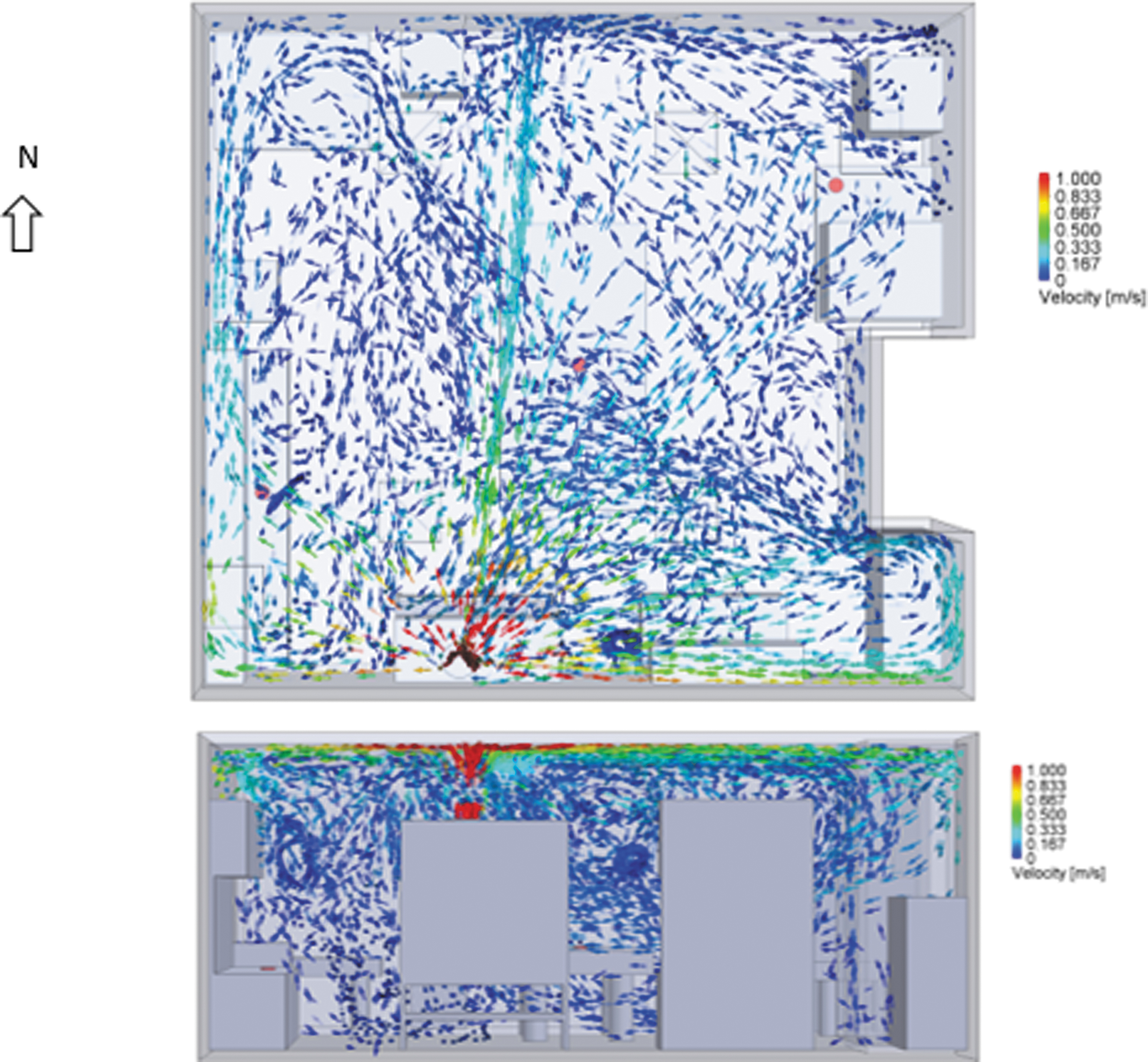
Plan view (top) and elevation view (bottom; looking north) of simulated steady-state flow patterns in the BSL-2 laboratory.

Transient Contaminant Concentrations

The transient airborne contaminant concentrations at the nine receptor locations are plotted in Figure 3 for the three contaminant source locations. Results show that the concentrations increase initially for several minutes as the contaminant plume disperses from the source. The concentrations eventually asymptote to steady-state values, but the normalized steady-state concentrations vary by nearly three orders of magnitude between ∼0.01 and 10 ppm.

Figure 3.

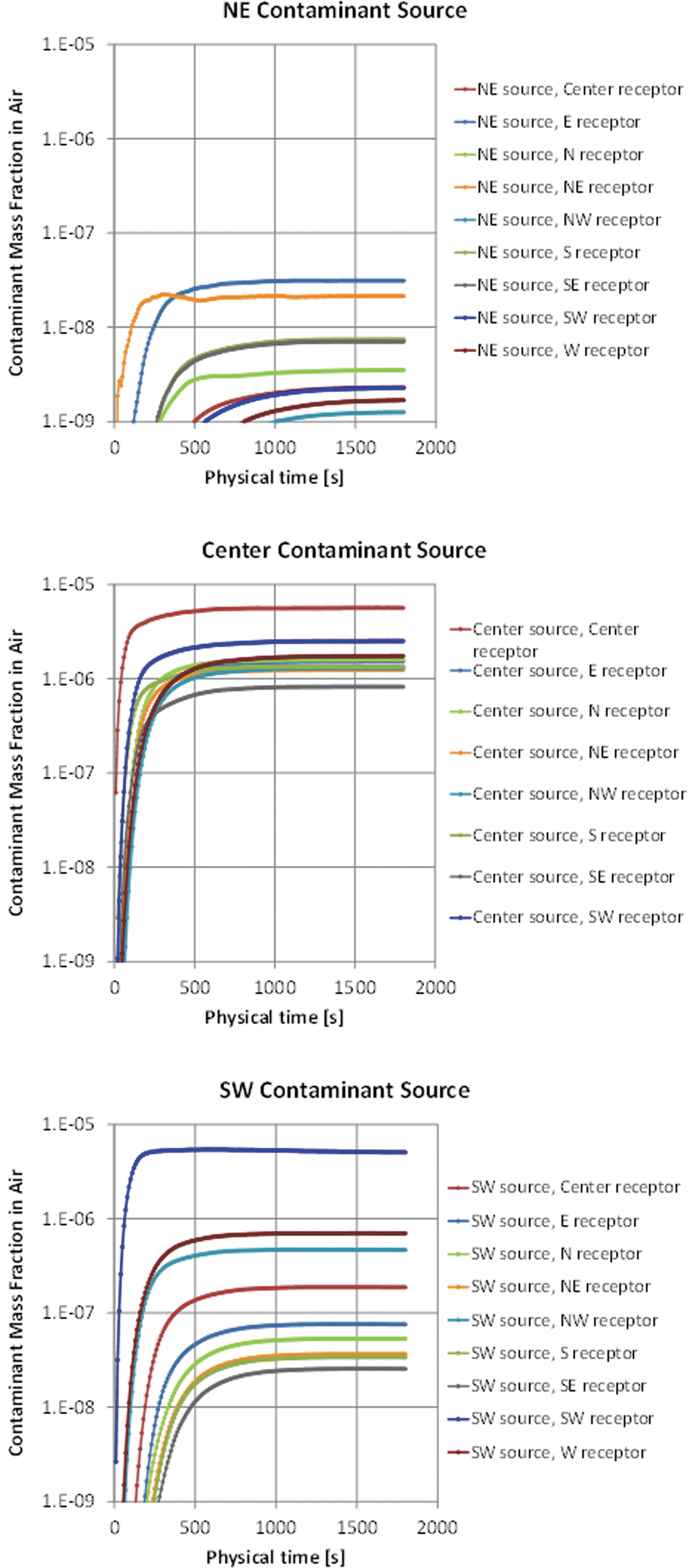
Top: Simulated contaminant concentrations as a function of time at nine locations for the NE release location. Middle: Simulated contaminant concentrations as a function of time at nine locations for the center release location. Bottom: Simulated contaminant concentrations as a function of time at nine locations for the SW release location.

The source located in the center of the room yields higher concentrations (∼1–10 ppm) on average throughout the room because it is further from any of the return vents and enables greater spreading of the contaminant throughout the room before being removed (Figure 3). The resulting concentrations from the center source are also more uniform than the other locations. At the NE and SW source locations, the contaminant has a direct path to the return vents located in the NE and SW corners of the ceiling. This tends to limit the contaminant plume to regions closer to the source, reducing concentrations in areas further away from the source. The SW source shows that the SW receptor location receives a high concentration due to its proximity to the source.

Figure 4 shows isosurfaces of the contaminant plume (at 1 ppm) at 1 and 15 min after initiation of release. The results show the trend in plume dispersion resulting from the different source locations as described earlier.

Figure 4.

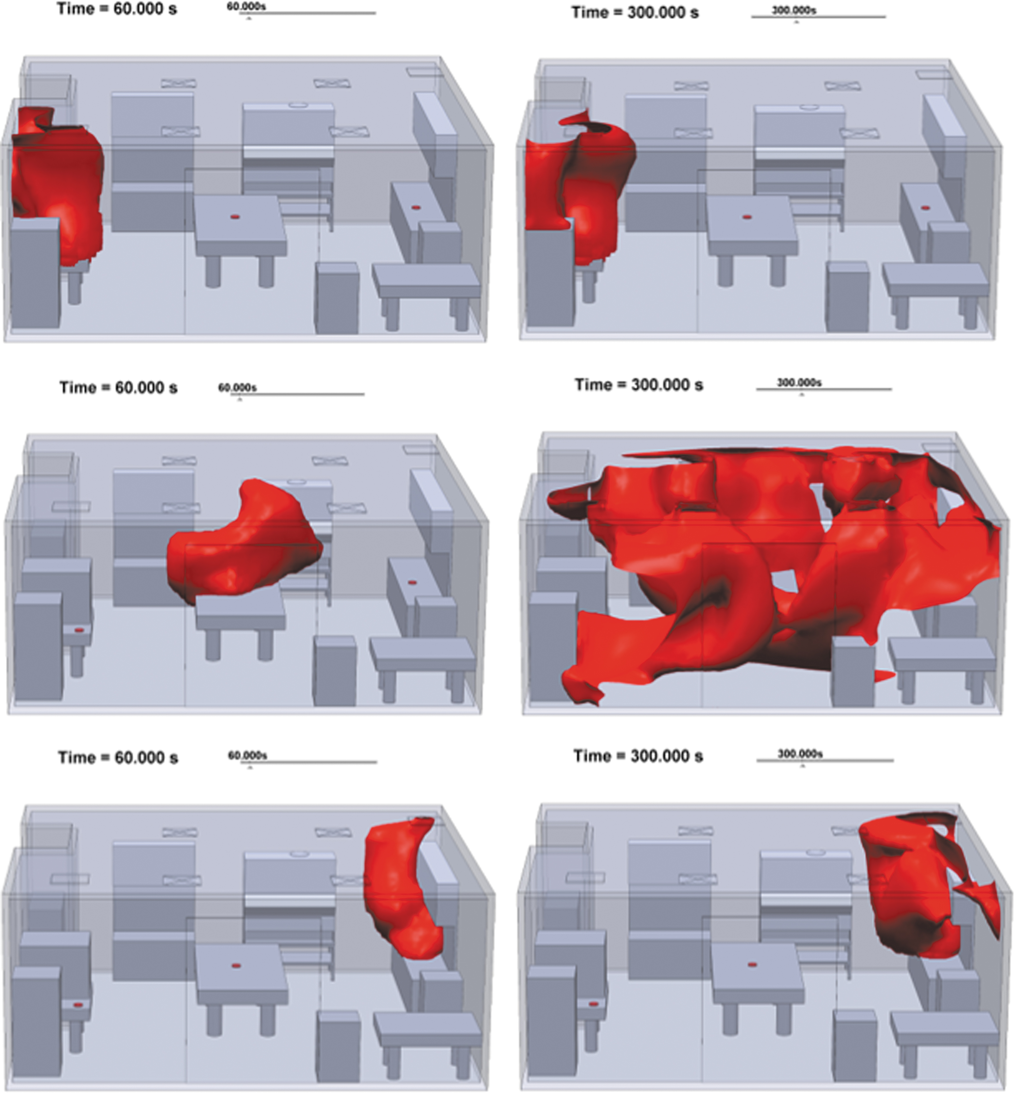
Top: Simulated contaminant isosurface (1 ppm) at 1 and 5 min looking south for the NE release location. Middle: Simulated contaminant isosurface (1 ppm) at 1 and 5 min looking south for the center release location. Bottom: Simulated contaminant isosurface (1 ppm) at 1 and 5 min looking south for the SW release location.

Time-Integrated Concentrations

Figure 5 shows the time-integrated concentrations normalized to the time-integrated source concentration (mass fraction = 1) after 30 min at the nine locations for the three source locations. Results are similar to the transient concentration plots. The normalized time-integrated concentrations are generally higher for the center release location due to its greater distance from the return vents, which promoted greater dispersion throughout the room (Figure 4). For a given source location, the exposures can vary by up to a couple orders of magnitude.

Figure 5.

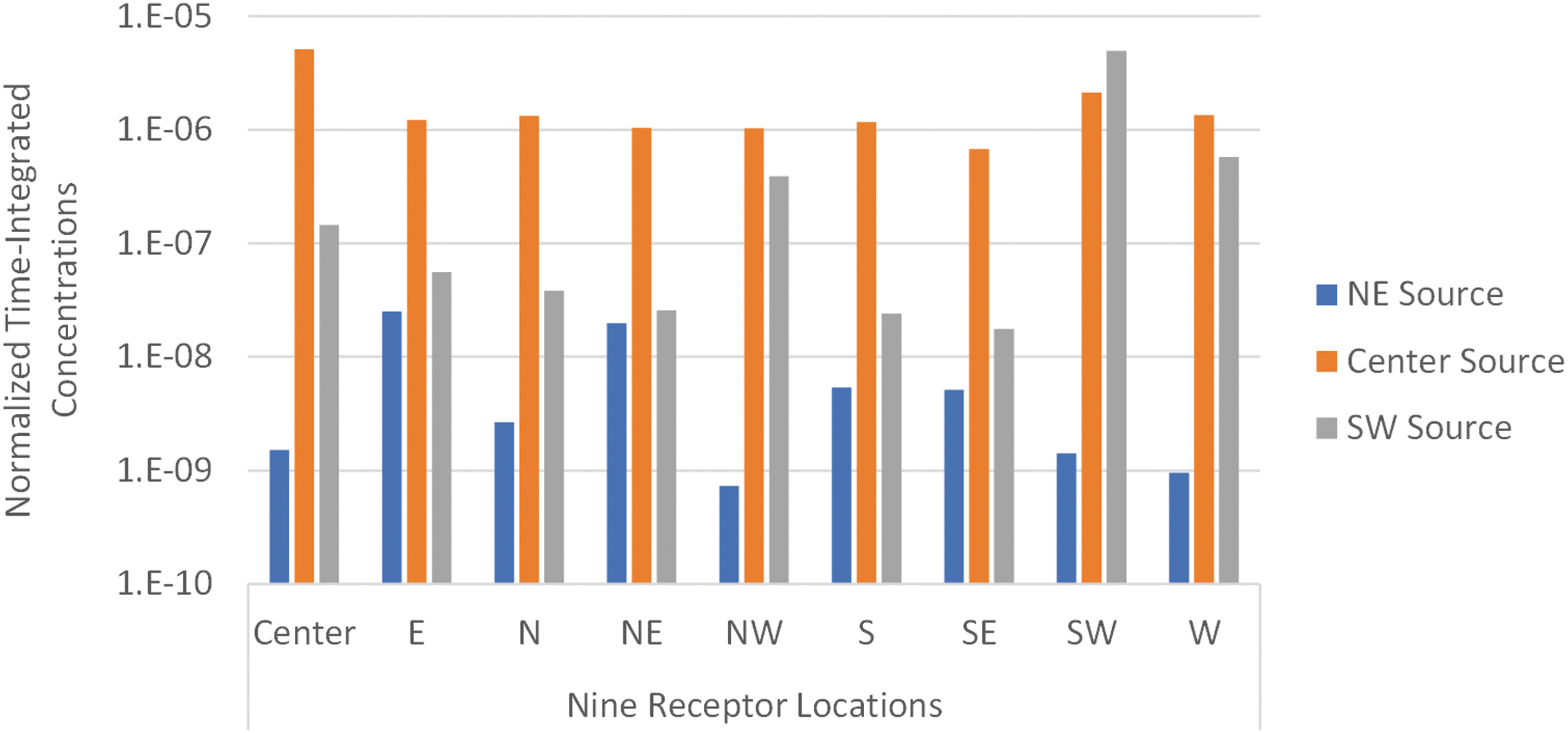
Simulated time-integrated concentrations normalized to the time-integrated source concentration (mass fraction = 1) after 30 min at the nine receptor locations for the three source locations.

Discussion

These preliminary CFD simulations show that laboratory ventilation configuration and contaminant source location can significantly impact airborne concentrations within the laboratory as measured at various locations in the room. Depending on the source location and airflow patterns, the transient and time-integrated concentrations were found to vary by several orders of magnitude in this example laboratory. Given that time-integrated concentration is closely related to inhalation exposure risks, these findings suggest these factors may warrant further exploration to understand the role they play in contributing to laboratory exposure risk. Although this initial study did not measure dose levels from laboratory procedures, it may be that certain combinations of biomaterials, laboratory manipulations, laboratory ventilation configuration, and worker handling protocols may present sufficient concern to warrant further study.

The CFD simulations confirmed expectations that contaminant plumes from sources located near a return vent (or exhaust like a fume hood or ventilated BSC) are more likely to be contained than sources that are far from the exhaust. Having a direct flow between the source and the exhaust (through-flow condition) may reduce potential exposures if individuals are outside the air flow path. Designing a BSL-2 room with ventilation and airflow patterns that maximize through-flow conditions to the return/exhaust vents and minimize dispersion and mixing throughout the room is recommended.

The results from this pilot study suggest CFD simulations may be helpful in assisting with characterizing the impacts of supply and return vent locations, room layout, and source locations on spatial and temporal contaminant concentrations. In addition, such simulations may aid in proper placement of contaminant sensors to provide additional characterization and monitoring of potential exposures in BSL-2 facilities.