
Abstract
Flash floods generated by runoff from abandoned spoil heaps have posed great risks to neighbouring areas but there has been little study on the process, so it is difficult to evaluate the effectiveness of runoff retention or detention measures. These events are likely to become more frequent in a future climate change scenario. To provide a means by which interested parties can study such events, including methods of mitigation, a computer modelling approach is proposed using free open-source software. Unlike conventional tools that solve the shallow water equations, the software tool uses a cellular automata approach to reduce the computational overhead. It is also easy to use so it is suitable for use by practitioners who are not hydrology experts. The method is illustrated by modelling a historical flood in the UK involving spoil heap runoff. Good correlation was observed between the characteristics of the actual and simulated flood event.
Keywords
Introduction
Water runoff during heavy rainfall events from the large mounds of waste rock at mine sites – which we refer to in this paper by the term ‘spoil heaps,’ as commonly used in England and Wales – is a recognised and not uncommon phenomenon, and several studies have investigated contributory factors. Hancock et al. (2003) concluded that the non-geomorphic profile of many spoil heaps exacerbates runoff, although this can be reduced by introducing concave slopes, which approximate to the lower reaches of natural hillsides. The absence of natural topsoil on spoil heaps contributes to runoff, although compaction of any topsoil which is present, sometimes caused by attempts at spoil heap remediation, is a further contributory factor (Haigh & Sanson 1999). Related to this, the geological nature of the spoil material is another factor that can increase runoff, even if topsoil is present. This is due to the breakdown of typical colliery spoil constituents, most commonly shale and mudstone, that can clog the pores in the soil (Haigh 1992). Runoff due to the lack of vegetation, or coverage by grass only, as opposed to bushes and/or trees, has been the subject of much research, for example by Haigh and Sansom (1999) and Moreno-de las Heras et al. (2009), although there is a degree to which any such lack of vegetation is secondary, resulting from the issues relating to the absence or compaction of topsoil, and its contamination by unfavourable rock types.
The majority of work on the consequences of runoff from spoil heaps has related to two adverse effects. First, the runoff waters can cause erosion of topsoil which, in turn, can impact spoil heap remediation measures, deposit silt in natural watercourses, and increase the potential for future runoff, thereby initiating a vicious cycle that exaggerates the effect (Kayet et al. 2018; Guo et al. 2020). Howard et al. (2011) investigated the efficiency of a variety of measures for preventing runoff and associated soil erosion, with particular reference to applying geomorphic principles. Second, the runoff waters can leach soluble minerals or their breakdown products from the spoil, thereby polluting the downstream watercourses and environment (Bayless and Olyphant 1993; Smith and Underwood 2000; Mayes et al. 2005; Lupankwa et al. 2006; Gozzard et al. 2009; Green 2009). However, very little work has been reported on the potential of runoff to cause flooding, and hence damage to local properties or disruption of services. Yet it is clear that this has already been an issue in the UK, the region in which the authors have by far the greatest access to historical information. Incidents include several unspecified cases of flooding in Meden Vale due to runoff from the spoil heaps of the closed Welbeck Colliery in Nottinghamshire (Mansfield District Council 2008), and at least two flood events in Blyth, Northumberland, as a result of runoff from the spoil heap of the former Isabella Colliery (Northumberland County Council 2020). Furthermore, it is speculated that the incidence of such flooding events will increase in a future climate change scenario in the UK and other areas, including many parts of Europe, where modelling shows a rising probability of more frequent extreme precipitation events (Rajczak et al. 2013; van Oldenborgh et al. 2015).
As reported in some of the previously cited work, a major contributory factor to runoff is the artificial characteristics of spoil heaps compared to naturally occurring hills. Because a high proportion of British spoil heaps were abandoned many years or decades ago, and many of these have been effectively restored, their characteristics will better resemble natural hills and they are, therefore, at a reduced risk from runoff. In regions where a large number of collieries are recently closed, or where restoration work such a vegetation of spoil heaps is not yet mature, it is hypothesised that the likelihood of flooding due to runoff will be significantly greater, and could pose a significant threat. In the light of this observation, research has been carried out into a method of assessing the risk potential of runoff-related flooding by computer simulation.
Modelling approach
Typically, flood modelling has relied on physical models that implement the shallow water equations (SWEs) (Dawson and Mirabito 2008), which are partial differential equations derived from the 3D Navier-Stokes equations. However, their solution requires significant computational resources. Much work has been carried out to reduce the computational overhead and/or improve performance, while maintaining an acceptable level of accuracy, by reducing the complexity of the equations and therefore the models. This is commonly achieved by approximating or neglecting some of the less significant terms in the equations. Examples of this approach include the JFLOW model (Bradbrook et al. 2004), the Urban Inundation Model (UIM) (Chen et al. 2007), and LISFLOOD-FP (Hunter et al. 2005; Bates et al. 2010). Other models do not employ a simplification of the SWEs but, instead, improve performance by using multi resolution grids (Hénonin et al. 2015), e.g. MIKE FLOOD – see (Labonté-Raymond et al. 2020) which illustrates its use in a mining context, or an irregular mesh, e.g. InfoWorks ICM (Innovyze 2022).
To accelerate simulations, flood modelling software based on solving the SWEs may use multi-cored processors and/or graphics processing units (GPUs) to achieve parallelism, i.e. to permit several operations to be carried out simultaneously. However, such physically based models are not always able to take full advantage of parallelism, because of their need for inherently sequential computations and, therefore, still pose performance challenges. Accordingly, either performance is poor or, if high speed operation is necessary, specialised and very expensive computing hardware is needed. In addition, the software is commonly intended for use by experts in hydrology with consequential ease-of-use issues for non-experts.
By way of contrast, it was an aim of the study reported here to use software that requires much lower computational resources, so it could be run on an ordinary PC, albeit probably high-end, instead of a very expensive and specialised workstation. It was also an objective to select software that is easy to use, so it can be utilised by mining professionals, environmental engineers, town planners, and others who are not hydrology experts.
Introduction to the flood modelling approach
Cellular automata method
In the light of the requirement for a low computational overhead, consideration was given to the more recent but less common category of flood modelling tools that employ cellular automata (CA). CAs can be in any number of dimensions but, for the purpose of flood modelling, a 2D CA would be used. An introduction to cellular automata – in the general sense rather than with specific reference to flood modelling – is provided by Delorme (1999). Put simply, though, a 2D CA requires that two-dimensional space is divided into cells, which are typically squares. Each cell can have a number of states which, in the case of flood modelling, would be the level of water in the cell. A CA also requires a definition of which cells are considered neighbours, and of the rules that define how the state of a cell changes from one time step to the next. Ideally, the transition rules are simple and use, as their input, the state of the cell itself and of its immediate neighbours. This approach is inherently much less demanding of computing resources than methods that involve solving partial differential equations.
Two CA flood modelling tools were identified, CA-ffé (Jamali et al. 2019) and CAFlood (Ghimire et al. 2013; Gibson et al. 2016; Webber et al. 2018; Gibson et al. 2020). The latter is free software, developed by two of the authors of this paper, and was selected for use here. The chosen open-source application implements the weighted CA flood rules (Guidolin et al. 2016) within the CADDIES framework.
A high-level summary of the internal workings of our chosen modelling tool is provided here. Calculation is carried out iteratively, for each spatial cell and for each time step. Accuracy increases by reducing the size of the cells and the time step, but this is at the expense of greater computing time. This description refers to Figure 1, which shows an area of ground three cells square.
Top-level view of the CADDIES approach to flood modelling. Images are available in colour online.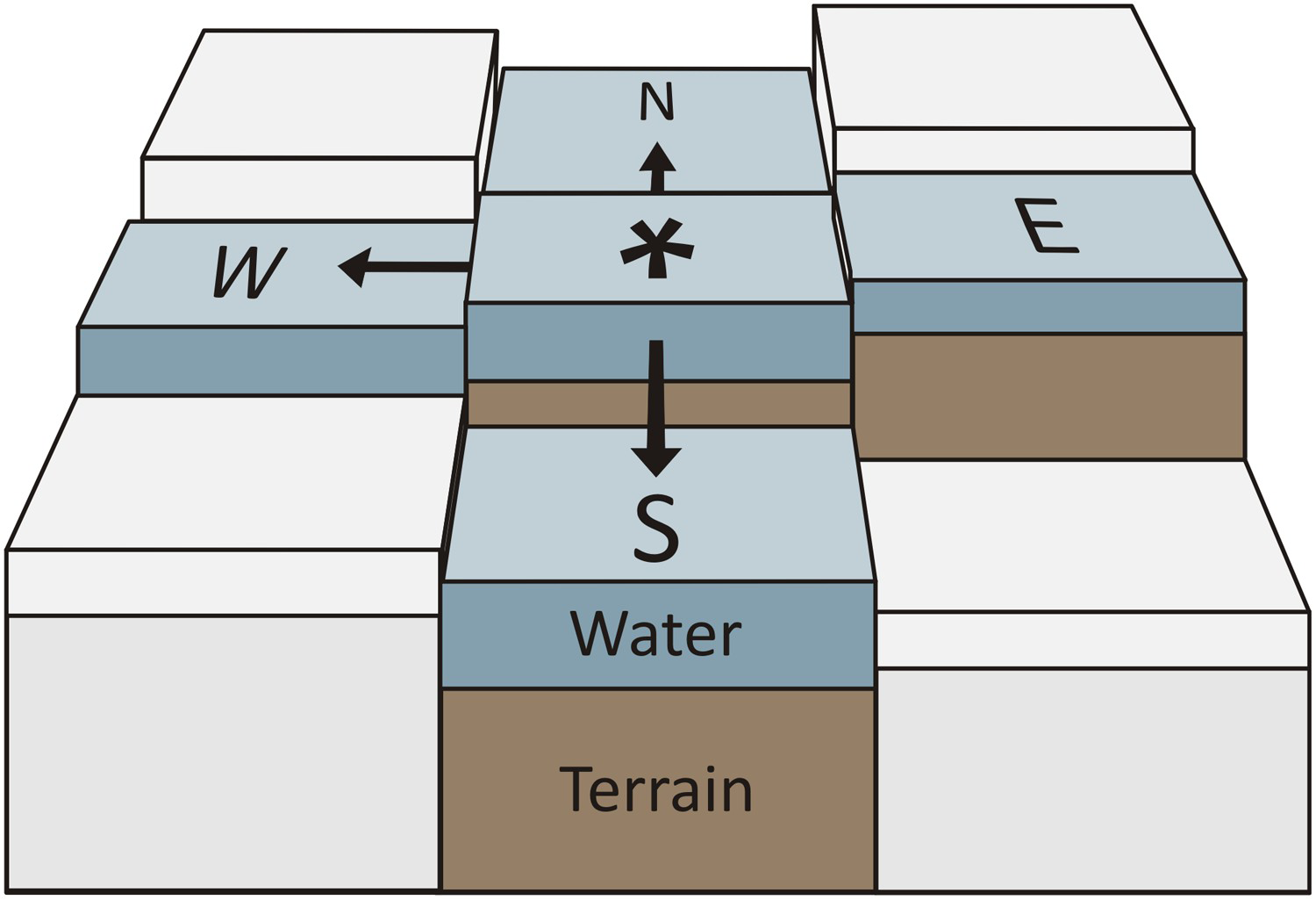
The so-called von Neumann neighbourhood is used, which means that the four cells directly north, south, west and east of a cell are considered its neighbours. In Figure 1, the cell being considered is marked with an asterisk, while the four neighbouring cells are marked with N, S, W and E. The other cells are not considered neighbours, so they are greyed out.
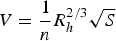
At each time step, the flow of water from each cell to its neighbours is calculated, depending on the level of water level at each cell, which is the sum of its terrain elevation and water depth. In Figure 1, water flows are shown using arrows, and it can be seen that there will be a flow to the north, south and west cells, because these have a lower water level, whereas the easterly neighbour has a higher water level. The flow of water is calculated using the empirical Manning Equation, which is based on Manning (1889), and which is defined as follows:
Handling infiltration
Infiltration, in this context, refers to absorption of rain water into the ground, a process that can lead to ground saturation, after which subsequent rainfall will remain on the surface and contribute to runoff. Traditionally, the changing soil saturation with time will reduce the actual infiltration rate. Green-Ampt or Horton's equations are used to describe the soil infiltration accurately, and include many more variables and require extra computational efforts to solve. In flood modelling, the temporal variation of infiltration has a minor influence on the surface runoff. Thus, in CAFlood, the water is allowed to infiltrate the soil up to a given rate that represents the soil's maximum infiltration capacity. This simplified approach is able to reflect the infiltration feature adequately without spending too much computing resources on analysing the minor phenomena.
To confirm the view that this simplified approach will not have a negative effect on spoil heap runoff modelling, a review was conducted of all available case studies in which the presence of a spoil heap was considered a contributory factor in a flood event. Eight such historical events were identified in the UK, although most of these were attributed to mechanisms other than runoff. All of these events occurred on a day of very high rainfall, as would be expected, but all of those events also occurred following a protracted period of high rainfall. A tentative conclusion was that flood events in the UK, and probably in other areas with a similar climate, usually occur when the ground is already fully saturated due to a long wet spell. However, it is possible that this observation could be more related to the fact that rainfall in the UK usually occurs over protracted periods, with isolated heavy rainstorms following a previous dry period being much less common.
To further assess the suitability of a modelling tool that does not handle variable infiltration, therefore, an investigation was conducted of the spoil heap saturation process and, therefore, of the transition from infiltration to runoff. Sherman and Musgrave (1942), Lv et al. (2020) and Woods et al. (2001) studied the evolution from infiltration to runoff from hills and spoil heaps during heavy rainfall events. All showed a very rapid transition, with a high proportion of rainfall being converted to runoff within a period of just 30 min. This is a relatively short period, compared to the duration of typical rainstorms that cause flooding in the UK. Therefore, assuming the heaps were fully-saturated during simulations would be acceptable, and therefore the infiltration could be neglected. In those rare cases where the heavy rainfall event followed a long dry period, the simulated period of rainfall could be reduced slightly to compensate for the short period of infiltration. The failure to model the saturation process was not, therefore, considered to be problematic, especially in areas with a North-western European climate, indeed there is evidence that it would fully meet the set objectives.
Modelling workflow
The easy useability for non-expert users was a key reason that a CA-based tool was chosen in preference to more conventional flood modelling tools. It is, therefore, appropriate to describe the steps involved in the modelling workflow to illustrate the inherent simplicity of the approach. This description is generic, although a few details, which relate to the particular modelling exercise presented here, appear later in the ‘Example Application’ section. It is pertinent to point out that some stages of the modelling approach, as described later, require the use of Geographical Information System (GIS) software, which can be thought of as a tool for digital map manipulation. The required GIS functions associated with a CAFlood modelling exercise are available in the open software QGIS, so this is the recommended GIS for input data preparation and output post-processing by non-expert users. Its suitability is evidenced by the fact that one of the authors of this paper, who had no previous experience of GIS software, was able to learn how to carry out all the necessary processing in just two days.
Data collection
The first steps involve obtaining the necessary input data, namely an elevation model, rainfall history, and surface roughness data.
The required elevation data is a Digital Terrain Model (DTM), which is freely available in some countries, although it might be necessary in other regions to use commercially available data. The Environment Agency's LiDAR data for England are freely available to the public and were used in this study. 1 m elevation resolution data is recommended, if available. Occasionally, data for the region around the spoil heap will be available at a mixture of resolutions. In such instances, terrain data processing would be required to create a merged dataset in which the higher resolution is used where available, with the gaps being filled with the lower resolution data. This is easily achievable in QGIS. In addition, for an initial scoping run, which is described below, 2 m resolution DTM is preferable to the highest 1 m resolution DTM for quicker analyses. It might also be necessary to use QGIS to merge DTM tiles to provide a single dataset for the region of interest, to crop an over-sized tile, and/or to convert the data to the necessary ASCII grid file (.ASC format).
Rainfall data is required from the closest weather station. Such data is freely available in some countries, although it might be necessary in other regions to use commercially available data. Hourly rainfall data is adequate, and this must be provided as a Comma-separated Values file (.CSV format) which can easily be created using spreadsheet software such as Excel.
A single value of the Manning's Roughness is applied to the entire area to reflect the spoil heap surface's influence on runoff propagation. A value can be estimated from visual observations of the spoil heap by consulting one of the many published tables such as the one by Oregon State University (undated).
Processing
Having assembled the necessary data, a simulation is carried out. However, it is recommended that this is conducted in two stages: (1) a scoping study, and (2) the main simulation. The scoping study will usually cover a larger area than the primary region of interest, and it will cover a much longer time period than the period of heavy rainfall. However, to reduce computing time, using a lower resolution DTM is recommended instead of the finest 1 m data which, ideally, should be used for the main run. The purpose of the scoping run is twofold. First, it reveals whether there are any substantial flows of water towards the major areas of flood accumulation other than runoff from the spoil heap. If any such flows are identified it would be necessary to study the region in more detail before concluding that any flooding is spoil heap related. If no such flows are identified, it is appropriate to continue with the main simulation. The second purpose of the scoping study is to identify the period of time during which flood levels continue to vary. Having made this determination, this is the period over which the higher resolution main simulation should be run. The modelling workflow is the same for both the scoping study and the main simulation except that the DTM will cover a larger area, ideally at a lower resolution to reduce processing time, and that different setup files will be used. The method is described in the following paragraphs.
As a word of introduction, CAFlood does not have a Graphical User Interface (GUI) so, rather than selecting commands from menus and on-screen buttons, it is driven by typing a textual command from the command line interface. The GUI approach, which is almost universal on Windows or macOS PCs, is considered to offer ease-of-use benefits but, in this instance, it is suggested that using the command line interface is much easier to learn than using a GUI. Specifically, a simulation is initiated by typing a single command, and all the necessary parameters and user preferences are supplied via a few setup files, which must be Comma-separated Values files (.CSV format) so they can easily be created using spreadsheet software such as Excel. In the simplest of cases, as used in the study described here, just three such setup files are required: (1) the main setup file, (2) a raster output setup file that defines the required variable (water flow angular velocity, water depth or water level, the latter being elevation plus water depth), and the period between raster outputs, and (3) a time plot output setup file that defines the required variable (water flow angular velocity, water depth or water level), the places of interest, and the period between time plot outputs. Full details, with examples, are provided in the CAFlood User Documentation (Guidolin et al. 2015), and in the case of many of the setup parameters, default values can usually be used.
Having obtained and, where necessary, pre-processed the elevation and rainfall data, and created the three setup files, a modelling run is initiated. Even though the CA approach is much more efficient than conventional flood modelling tools in terms of its requirement for computing resources, there will then be a significant delay, often measured in hours, before the run terminates. On termination, it is preferable to process the output data files for ease of interpretation as described below.
There will, typically, be several raster output files – which are water flow, depth or level maps – the number of which depends on the contents of the raster output setup file, but they can all be processed in the same way. Each file, which will be an ASCII grid file (.ASC format), should be imported into QGIS as a raster layer, and the display options adjusted to define the required display options. In addition to saving the result as a QGIS project file (.QGZ format) for quick and easy future access, exporting it as an image file (e.g..TIF,.PNG,.JPG format) is also recommended.
There will, typically, be one or more time plot output files, which will be a Comma-separated Values files (.CSV format), which are most easily processed by being imported into spreadsheet software such as Excel, where it is a straightforward exercise to display this data as a line graph against time. In addition to saving the result as an Excel file (.XLS format) for quick and easy future access, the graph can be copied and pasted into many applications.
The workflow for simulating a flood event is summarised as a flow diagram in Figure 2. This includes all the processes described above, which are shown as blue rectangles, and all the data files, which are shown as yellow cylinders. Note that the roughness data does not appear in the flow diagram because it is just a single value which is entered into the main setup file. Although the diagram initially looks quite complicated, that view is rather misleading because each process is simple and largely independent of the others.
Flow diagram of the simulation workflow. Images are available in colour online.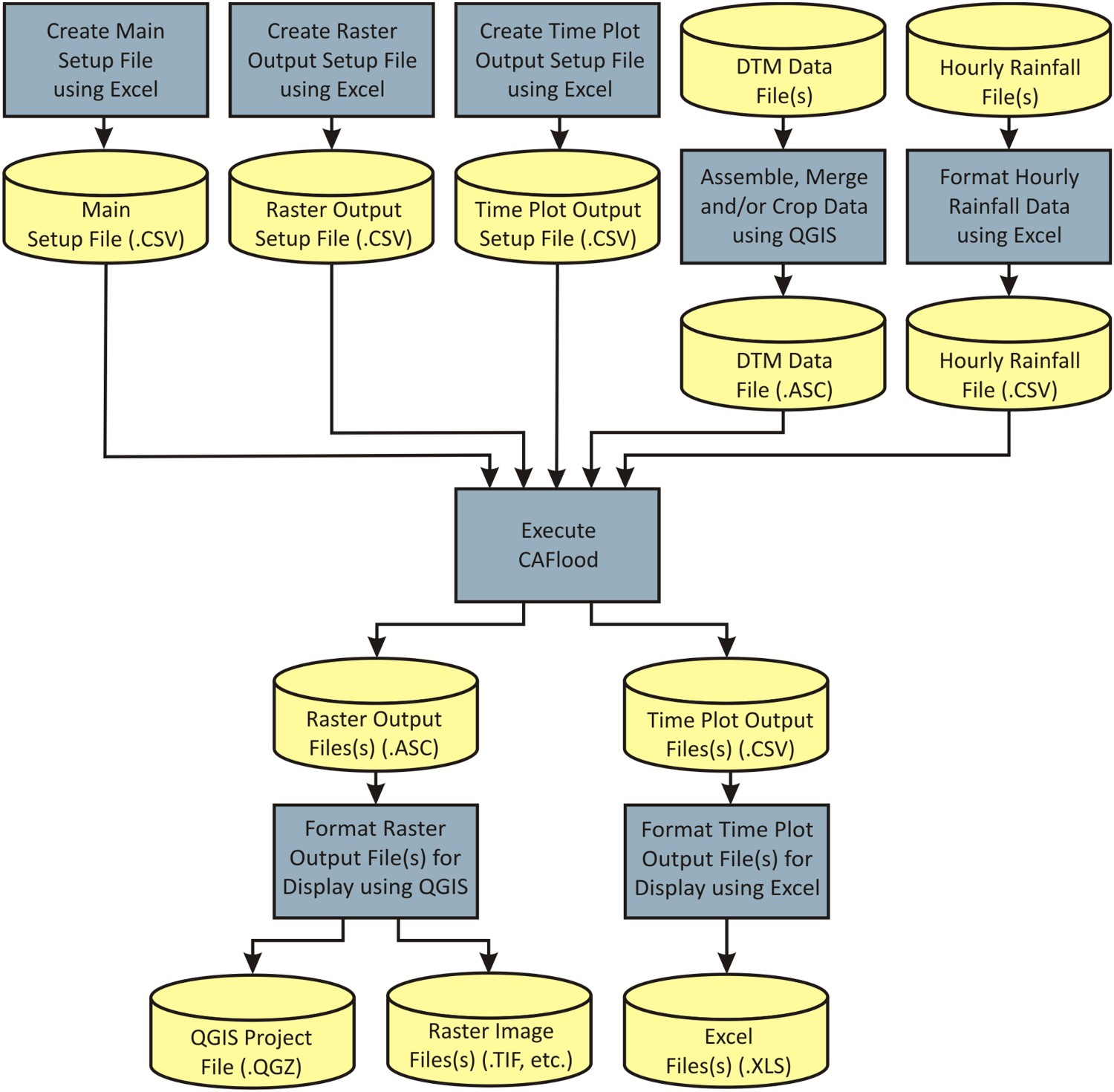
Example application
Historical event
Several verification studies of CAFlood have been published, showing comparable performance to conventional physical model-based flood modelling tools in urban environments (Gibson et al. 2016; Guidolin et al. 2016). However, to investigate its suitability for modelling flooding due to runoff from spoil heaps, a verification study relating to this scenario was carried out. This was conducted by modelling a historic flood event for which the following details were provided by Northumberland County Council (2020) in response to a Freedom of Information request relating to flood events in Northumberland.
We only know of one location where flooding can be attributed to old coal mine spoil heaps. This is the Isabella cutting, Blyth. At this location surface water falls onto and off the soil heap and collects in a disused railway line. The rainwater here travels in a northerly direction towards Malvins Road where flooding occurs. The flooding is only confined to the railway cutting. Flooding of this area is known to have occurred on 28 June 2012 and in 2015. (exact date – unknown)
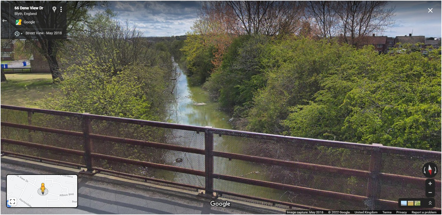
The described water flows are shown superimposed on satellite imagery of the area in Figure 3 (the locations numbered 1, 2 and 3 are referred to later), and flooding in the abandoned railway cutting, as seen looking south from the bridge on Albion Way, can be seen in Figure 4. Although this photograph is of a more recent flood event than the one cited by Northumberland County Council for which photography cannot be reproduced, it is understood to be representative of the several instances of flooding that have occurred at this locality, including the particular one reported by Northumberland County Council.
Water flows and flood extent as described by Northumberland County Council (2020). Images are available in colour online. Flooding in abandoned railway cutting due to spoil heap runoff. Images are available in colour online.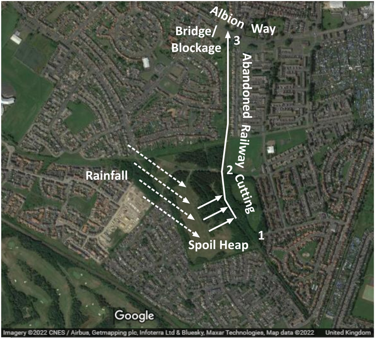
Modelling exercise
A Digital Terrain Model (DTM), of the region was obtained from the UK Environment Agency. 1 m resolution data was used where available but, since the coverage was not complete, 2 m resolution data was used to fill in any gaps, using QGIS to merge the two datasets. Hourly rainfall data was obtained from the UK Met Office for 28 June 2012, from the closest weather station, Albemarle, which is 27 km from the area of interest. This showed a rainfall event that involved 25.4 mm of precipitation, mostly within a five-hour period, with a maximum hourly value of 18.6 mm. A value for the Manning Roughness of 0.035 was estimated from visual observations of the spoil heap by consulting the published table at (Oregon State University, (undated)). In accordance with the previous discussion on ground infiltration, and the evolution from infiltration to runoff, a value of zero was used as the infiltration rate.
Prior to the main high-resolution simulation run, a lower resolution scoping study was carried out using 2 m elevation data for an area larger than the region of particular interest, for the period of time that covered the rainfall event and several hours afterwards. No secondary flows of water into the area of flooding were identified, thereby providing confidence in the applicability of running the main higher resolution simulation over a more targeted area. It was also noted that water levels and extent did not change significantly after 40,000 s (about 666 min) from the first rainfall, this being approximately 360 min after the end of the rainfall event. Accordingly, a simulation period of 700 min was used in the main higher resolution run.
Graphical representations of key elements of the modelling output are reproduced here. Figure 5 shows the evolution of water depths at three points in the railway cutting, as identified by the location numbers in Figure 3 (i.e. Figures 1–3 that appear to the left of the wording ‘Abandoned Railway Cutting’), together with the input rainfall data. It shows a final water depth of about 1.2 m at the northern end of the cutting at the Albion Way bridge where the cutting is blocked.
Rainfall and water depth vs. time in the abandoned railway cutting. Images are available in colour online.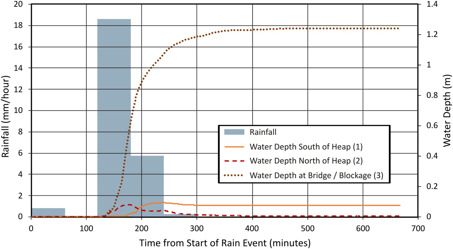
Another important output is a flood depth map at the end of the simulation period, which is reproduced as Figure 6, and covers approximately the same area as Figure 3, and with the main area of flooding in the railway cutting shown at a larger scale. It shows that, when water levels had stabilised, flooding extended south from the Albion Way bridge for at least 300 m.
Flood depth at the end of the simulation period. Images are available in colour online.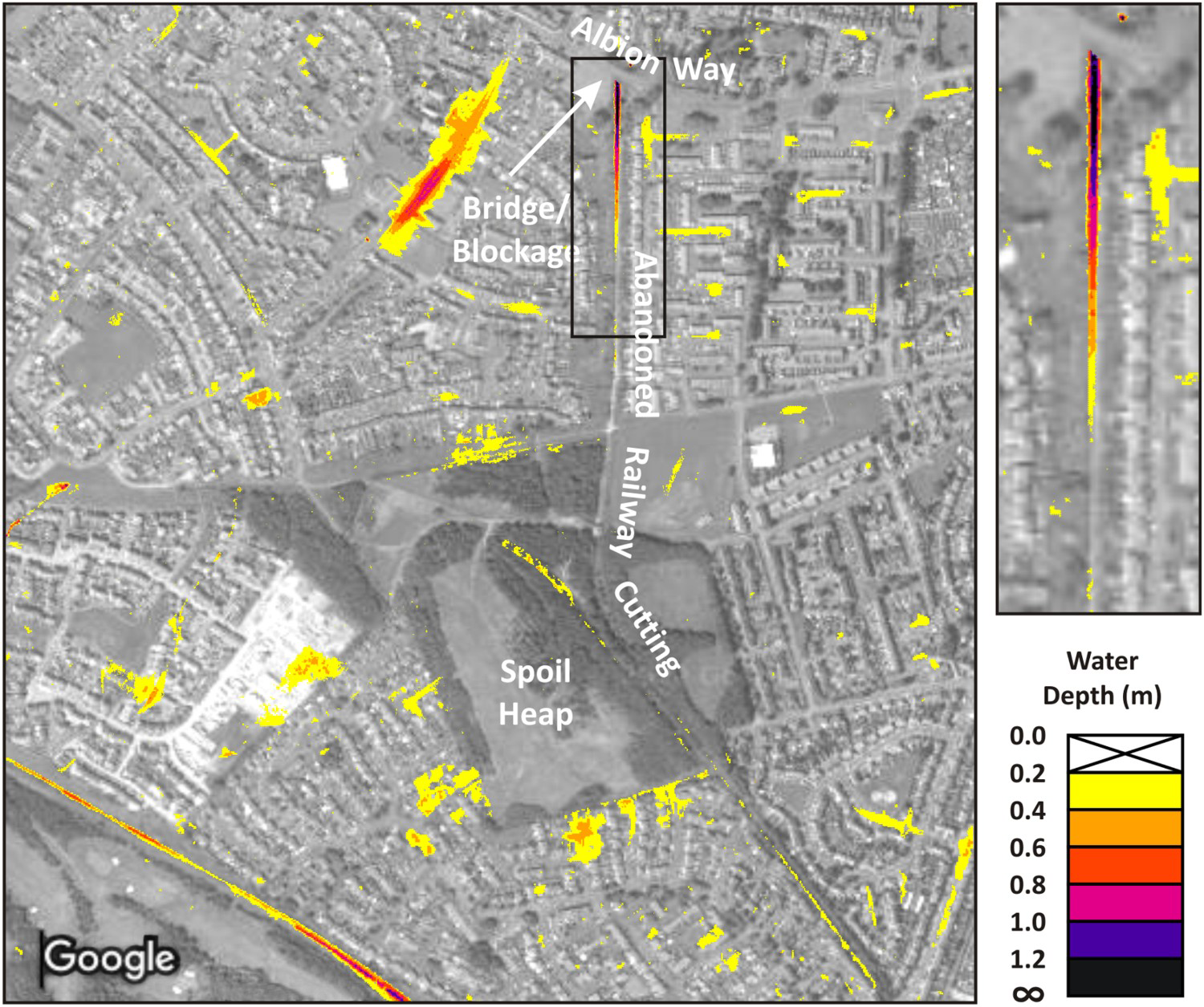
The simulation results are consistent with the verbal description provided by Northumberland County Council and the unpublished photographs that were shared by Northumberland County Council. The photograph of a more recent flood event, which is reproduced as Figure 4, and which shows the affected area better than the photographs provided by Northumberland County Council, is understood to be similar to the simulated event, and is also consistent with the simulation results.
The main simulation run took 2 h 23 min. The hardware was a PC fitted with a NVIDIA K20c Tesla GPU accelerator. This card has a NVIDIA CUDA GPU chip with 2496 cores, a processor clock rate of 706 MHz, and a memory clock rate of 2.6 GHz. It offers a peak double precision floating point performance of 1.17 teraflops and a peak single precision floating point performance of 3.52 teraflops. It is estimated that the computation would take about 10 times longer to run on a reasonably high-end desktop PC with no GPU accelerator, but with a several core Intel Core i7 processor. This is considered feasible for carrying out runs over a weekend, or perhaps overnight if only light use is made of the PC the following morning.
Simulating future events
To illustrate the use of this technique for investigating the flood risk in a future climate change scenario, a further simulation was carried out of the same site using modelled rainfall data for a future extreme rainfall event. Rainfall data was obtained from three climate models within the EURO-CORDEX 11 project (Jacob et al. 2014), namely CNRM-CM5, EC-Earth and HadGEM2-ES. In CORDEDX-11, general circulation models are dynamically downscaled by regional climate models over Europe with a horizontal resolution of 0.11 degrees (∼12.5 km). Euro-CORDEX is one of the most commonly used models for developing climate projections for use in impact and adaptation studies. Daily precipitation data was downloaded from the CEDA portal for the RCP4.5 scenario for the period 1 January 2046–31 December 2050. From this specific data, a grid was extracted for the area around Blyth where the Isabella Tip is located. Daily modelled rainfall data provides information on peak values and their frequency of occurrence. The modelled data identified the wettest day, with 45 mm in a 24-hour period, in September 2048, this being in the CNRM-CM5 model. It should be recognised that no significance can be assigned to the specific date chosen for the simulation study – it only represents a possible future extreme rainfall event. Although hourly rainfall data can also be obtained, again this can only show likely trends, and no significance can be assigned to particular times within a 24-hour period. For this reason, rather than using modelled hourly rainfall data, the rain profile of the historical rainfall event was scaled up to give the modelled 45 mm daily rainfall. This approach makes comparisons more meaningful. The simulation results were similar to those of the historical flood event, although the depth of water at the northern end of the railway cutting increased to a maximum of approximately 2.0 m.
Conclusions
A study has been undertaken of methods which allow the flood risk due to runoff from spoil heaps during heavy rainfall events to be investigated by computer simulation. In particular, it was an aim to base this study on the use of a tool which would be applicable for use by mining professionals, environmental engineers, town planners, and others who are not hydrology experts. The chosen method involves the application of a free flood modelling tool called CAFlood which, unlike conventional flood modelling tools that solve partial differential equations, uses cellular automata technology to reduce the requirement for high-performance computing facilities. Coupled with its ease-of-use, it is considered that this will make such studies practical for non-expert practitioners who do not have access to specialist high-performance workstations.
The approach has been verified by conducting a simulation involving an abandoned spoil heap in Blyth, Northumberland, UK, that has been the subject of several historical flood events due to runoff from the spoil heap. The simulation results were in accordance with a verbal description of one such flood event provided by local authority engineers, and of photographs of the extent of the flood.
It is anticipated that the requirement for such a capability will increase due to more extreme rainfall events in the future, as a result of climate change in many parts of the world. However, as part of the planning process for handling abandoned spoil heaps, there is benefit in carrying out modelling exercises today using future rainfall data obtained from climate models. Indeed, such an exercise was carried out on the same spoil heap that was used to verify the modelling approach, an exercise that confirmed the expectation that future flood events are likely to be more severe.
The method described here is also recommended for use in modelling studies for investigating the impact of possible spoil heap mitigation measures to reduce the flood risk. Included here, for example, could be investigations of the impact of different vegetation regimes on the spoil heap and of upgrading the drainage systems associated with spoil heap runoff.
Footnotes
Disclosure statement
No potential conflict of interest was reported by the author(s).