Sage Journals: Discover world-class research

Abstract

We present word frequencies based on subtitles of British television programmes. We show that the SUBTLEX-UK word frequencies explain more of the variance in the lexical decision times of the British Lexicon Project than the word frequencies based on the British National Corpus and the SUBTLEX-US frequencies. In addition to the word form frequencies, we also present measures of contextual diversity part-of-speech specific word frequencies, word frequencies in children programmes, and word bigram frequencies, giving researchers of British English access to the full range of norms recently made available for other languages. Finally, we introduce a new measure of word frequency, the Zipf scale, which we hope will stop the current misunderstandings of the word frequency effect.

Keywords

Word frequency Visual word recognition Zipf scale

Word frequency arguably is the most important variable in word recognition research (Brysbaert, Buchmeier, et al., 2011). Words that are often encountered are processed faster than words that are rarely encountered. Figure 1 shows the course of the word frequency effect. It includes mean standardized reaction times (z-values) for samples of 1000 words going from an average frequency of 0.06 per million words (a log10 value of −1.2) to an average frequency of nearly 1000 per million words (a log10 value of nearly 3.0). The reaction times come from the English Lexicon Project (ELP; circles; Balota et al., 2007) and the British Lexicon Project (BLP; squares; Keuleers, Lacey, Rastle, & Brysbaert, 2012), which contain lexical decision times to over 40 thousand words of American English (ELP) or over 28 thousand monosyllabic and disyllabic words of British English (BLP). The word frequencies come from the British National Corpus (BNC; Kilgarriff, 2006), a 100-million-word collection of samples of mostly written and some spoken language from a wide range of sources, collected between 1991 and 1994 and designed to represent a wide cross-section of British English at that time. Another database of word frequency norms often used for British English is the CELEX lexical database (Baayen, Piepenbrock, & Gulikers, 1995), based on a corpus of 17.9 million words assembled along the same criteria as those for the BNC.
Figure 1.
The course of the word frequency effect in mean standarized reaction times from the British Lexicon Project (squares) and the English Lexicon Project (circles). The standard errors are represented by whiskers.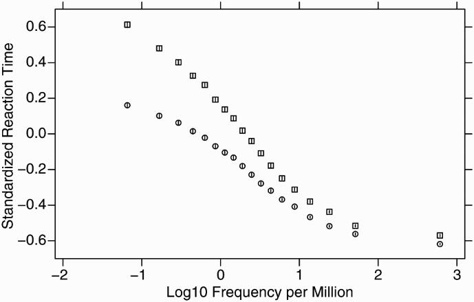

Research in American English and other languages has suggested that word frequencies based on film and television subtitles are better predictors of word processing times than word frequencies based on books and other written sources (Brysbaert, Buchmeier, et al., 2011; Brysbaert, Keuleers, & New, 2011; Brysbaert & New, 2009; Cai & Brysbaert, 2010; Cuetos, Glez-Nosti, Barbon, & Brysbaert, 2011; Dimitropoulou, Duñabeitia, Avilés, Corral, & Carreiras, 2010; Ferrand et al., 2010; Keuleers, Brysbaert, & New, 2010; New, Brysbaert, Veronis, & Pallier, 2007). This is an important finding, because the more variance can be explained by word frequency the fewer other variables are needed to account for word processing times. Brysbaert and Cortese (2011), for example, found that word familiarity did not explain much extra variance in lexical decision times to monosyllabic English words when the SUBTLEX-US subtitle frequency measure was used (Brysbaert & New, 2009) instead of a commonly used, outdated frequency measure based on a small corpus of written sources (Kučera & Francis, 1967).

Although word frequency estimates based on American subtitles can be used (and have been used) in British word recognition research, some precision is lost, because some words have a different spelling (e.g., labor vs. labour) or a different meaning (e.g., biscuits, pants) in the two languages. The divergences between American and British word usage imply that British researchers should limit their research to the words fully shared among the languages if they use American subtitle frequencies. Otherwise, their findings risk overestimating the impact of nonfrequency variables, such as age of acquisition, word familiarity, word length, or similarity to other words. Suboptimal frequency estimates also increase the risk of stimulus selection errors. This will be the case when words must be selected on the basis of frequency information (e.g., words having different numbers of closely resembling words, so-called orthographic neighbours, with higher frequencies) or when words of different conditions must be matched on frequency (e.g., highly emotional words vs. neutral words).

To address the limitations that researchers working with British English are confronted with, we decided to collect subtitle-based UK word frequency norms. In addition, because we were able to directly capture the subtitles from a variety of television programmes, for the first time we also collected subtitle frequencies from channels specifically aimed at children. Below we describe the collection of the data, the summary statistics calculated, and the first validation studies we ran.

Method

Corpus collection

In line with UK regulations, since 2008 the British Broadcasting Corporation (BBC) subtitles all scheduled programmes on its main channels, to help the hearing impaired.¹ These subtitles are not broadcasted through the main channel, but can be superimposed on the programme by those who wish so (e.g., by using Teletext). To have the widest possible range of language input, we collected the words and word pairs of the subtitles from nine channels (BBC1–BBC4, BBC News, BBC Parliament, BBC HD, CBeebies, and CBBC) broadcasted over a period of three years (January 2010–December 2012). Of these channels, BBC1 is the most popular and extensive (aimed at all types of audiences). The other channels have more limited hours. Of further interest is that the CBeebies channel is meant for preschool children (0–6 years) and the CBBC channel for primary school children (6–12 years). This allowed us to compile frequency norms for these groups.

Notwithstanding the provisions relating to “fair dealing” provided under Section 29 of the Copyright Designs & Patents Act 1988 (Government United Kingdom, 1988), the full textual content of the relevant subtitles was not stored or reproduced for the purpose of this research. A count of individual words and consecutive words was undertaken, obtainable from public transmissions. The method employed does not detract from or otherwise undermine the value of this evaluative work.

Text cleaning

The broadcasts were cleaned semiautomatically for doubles (programme repeats) and subtitle-related information not broadcasted to the viewers. Also the parts of the subtitles not related to the conversation were eliminated (e.g., the words “silence” or “thunder” to describe the ongoing scene; these are usually presented in upper case, or in a different font or colour in the subtitle). After the cleaning we obtained a total of 201.7 million words, coming from 45,099 different broadcasts. This is larger than the other existing subtitle corpora (Brysbaert & New, 2009; Cai & Brysbaert, 2010; Cuetos et al., 2011; Dimitropoulou et al., 2010; Keuleers et al., 2010)² and allowed us to calculate more precise parts-of-speech dependent frequencies and word bigrams.

Word Frequency Measures

Word frequency counts

A first decision to be made was what to do with hyphenated words. In British English, words are often hyphenated when they function as adjectives. So, a potion that saves lives can be described as “a life-saving potion”. This phrase could be counted as consisting of three word types (a, life-saving, potion) or four word types (a, life, saving, potion). The problem was particularly relevant for the BBC subtitles, because nearly one out of four word types contained a hyphen in the first analysis of the data. The vast majority of these hyphenated entries were of low frequency (fewer than 100 observations on a total of 200 million words). Because there are no a priori considerations about how to handle this finding (also because there is quite some individual variability in the use of hyphens; Kuperman & Bertram, 2013), we decided to use a pragmatic criterion and looked at which word frequencies correlated most with the 28 thousand lexical decision times of the BLP (Keuleers et al., 2012). As this clearly favoured the dehyphenated word frequencies (a difference in variance explained of 5%), we decided to dehyphenate the data before counting the words.³

The dehyphenated subtitles resulted in a total of 332,987 different word types for a total of 201,712,237 tokens. Of these, 31,368 types were in the CBeebies subtitles with a total of 5,860,275 tokens, and 70,755 types were in the CBBC subtitles with a total of 13,644,165 tokens. Because the vast majority of words observed in a single broadcast were typos and other nonword-like structures (like “aaaarrrrgh” or “zzzzzzzzzzzz”), we decided to take out all entries observed in a single broadcast only. This reduced the number of types to 159,235 with a total token count of 201,335,638 for the complete corpus, 5,848,083 for the CBeebies subcorpus (27,236 types), and 13,612,278 for the CBBC subcorpus (58,691 types).

A standardized frequency measure: The Zipf scale

Although the frequency counts are the most versatile measure (as will become clear later, when we calculate all types of derived measures), they have one big disadvantage. The interpretation of the frequency measure depends on the size of the corpus. Therefore, authors have looked for a standardized frequency measure, an index with the same interpretation across all corpora collected.

Thus far, the most popular standardized frequency measure has been frequency per million words (fpmw). It is the frequency measure that we made available in our previous work on subtitle frequencies as well. However, we increasingly noticed that this measure leads to an incorrect understanding of the word frequency effect.

Because their corpus contained only 1 million words, the lowest value in the word frequencies made available by Kučera and Francis (1967) was 1 fpmw. This contributed to the assumption that 1 fpmw is the lowest possible frequency. Obviously, this is no longer the case for larger corpora. As it happens, about 80% of the word types in SUBTLEX-UK have a frequency of less than 1 fpmw (i.e., fewer than 200 occurrences in all broadcasts). Second, as shown in Figure 1, nearly half of the word frequency effect is situated below 1 fpmw, and there is very little difference above 10 fpmw. The frequency effect of lexical decision times between 0.1 fpmw and 1 fpmw is equal to or larger than the effect between 1 fpmw and 10 fpmw. A logarithmic transformation of frequency measures, as is routinely performed, alleviates this problem. However, the logarithms of fpmw become negative for frequencies lower than 1 (as again shown in Figure 1), which uninformed users tend to avoid. Because of these properties, fpmw as a standardized measure puts users on the wrong foot.

To make the word frequency effect easier to understand, one needs a scale with the following properties: (1)
It should be a logarithmic scale (e.g., like the decibel scale of sound loudness).
(2)
It should have relatively few points, without negative values (e.g., like a typical Likert rating scale, from 1 to 7).
(3)
The middle of the scale should separate the low-frequency words from the high-frequency words.
(4)
The scale should have a straightforward unit.

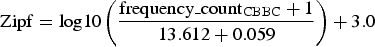
Once we know what the scale should look like, it is not so difficult to come up with a good transformation. In particular, when we take the log10 of the frequency per billion words (rather than fpmw), the scale fulfils the first three requirements. To meet the last requirement, we propose to call the new scale the Zipf scale, after the American linguist George Kingsley Zipf (1902–1950) who first thoroughly analysed the regularities of word frequency distribution and formulated a law (Zipf, 1949), which was later named after him. The unit then becomes the Zipf.

The Zipf scale is a logarithmic scale, like the decibel scale of sound intensity, and roughly goes from 1 (very-low-frequency words) to 6 (very-high-frequency content words) or 7 (a few function words, pronouns, and verb forms like “have”). The calculation of Zipf values is easy as it equals log10 (frequency per billion words) or log10 (frequency per million words) + 3. So, a Zipf value of 1 corresponds to words with frequencies of 1 per 100 million words, a Zipf value of 2 corresponds to words with frequencies of 1 per 10 million words, a Zipf value of 3 corresponds to words with frequencies of 1 per million words, and so on.

Table 1 summarizes the information. It also helps to clear one more misunderstandings about word frequencies among psycholinguists, namely that words with frequencies below 1 fpmw are too uncommon to be known. There are hundreds of derived and inflected word forms and even lemmas with frequencies of lower than 0.1 fpmw that are perfectly known, as can be seen in Table 1. Content words rarely have a Zipf value higher than 6, so that for most practical research purposes, the Zipf scale will be a scale from 1 to 6 with the tipping point from low frequency to high frequency between 3 and 4.
Table 1.
The Zipf scale of word frequency

Zipf value fpmw Examples

1 0.01 antifungal, bioengineering, farsighted, harelip, proofread

2 0.1 airstream, doorkeeper, neckwear, outsized, sunshade

3 1 beanstalk, cornerstone, dumpling, insatiable, perpetrator

4 10 dirt, fantasy, muffin, offensive, transition, widespread

5 100 basically, bedroom, drive, issues, period, spot, worse

6 1000 day, great, other, should, something, work, years

7 10,000 and, for, have, I, on, the, this, that, you

Note: The Zipf scale is a word frequency scale going from 1 to 7. Words with Zipf values of 3 or lower are low-frequency words; words with Zipf values of 4 and higher are high-frequency words. Examples are based on the SUBTLEX-UK word frequencies. fpmw = frequency per million words.

One more addition that is of interest for the Zipf scale is the possibility to include words with frequency counts of 0 (i.e., words not observed in the corpus). Although these words are less common in large corpora, they are by no means absent. Such words pose a problem for the Zipf scale as a result of the logarithmic transformation (given that the logarithm of 0 is minus infinity). In a recent review, Brysbaert and Diependaele (2013) concluded that the best way to deal with 0 word frequencies is the Laplace transformation. Rather than working with the raw frequency counts, one works with the frequency counts + 1. This means that all frequency values are (slightly) elevated. The proper application of the algorithm also implies that the theoretical size of the corpus is a little larger than the actual size, because one is leaving room for N unobserved word types with frequency 1. N is the number of word types in the frequency list. So, for the full corpus the Laplace transformation assumes that there are 159,235 unobserved word types extra in the language, all with a frequency of 1.

In practice, the following equation is needed to calculate the Zipf values on the basis of the frequency counts of the total corpus:
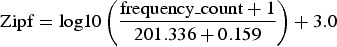
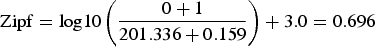
$Zipf = \log 10 (\frac{frequency_count + 1}{201.336 + 0.159}) + 3.0$

The values in the denominator are the size of the corpus in millions plus the number of word types in millions. Specifically, the Zipf value of an unobserved word type will be:
$Zipf = \log 10 (\frac{0 + 1}{201.336 + 0.159}) + 3.0 = 0.696$

The Zipf value of a word type observed once in the complete corpus will be 0.997; that of a word observed 10 times will be 1.737, and so on.

To calculate the Zipf values for the CBeebies corpus, we have to use the following equation:
$Zipf = \log 10 (\frac{frequency_{count}_{CBeebies} + 1}{5.848 + . 027}) + 3.0$
For the CBBC subcorpus the equation is
$Zipf = \log 10 (\frac{frequency_{count}_{CBBC} + 1}{13.612 + 0.059}) + 3.0$

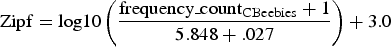
Specifically, this means that words with a 0 frequency in the CBeebies corpus get a Zipf value of 2.231; those with a 0 frequency in the CBBC corpus get a Zipf value of 1.864. The higher values for unobserved word types are due to the smaller sizes of the corpora and also mean that one should be sensible in their use. There is no point in blindly using these values for all missing words in the lists, as one assumes that the missing words are known to preschoolers (CBeebies) or primary school children (CBBC). As we see below, this may be one reason why the childhood frequencies are not correlating very well with the lexical decision times of the British Lexicon Project when calculated across all words.

To give readers a better feeling for the Zipf scale, Table 2 tabulates the summary statistics of the Zipf values used in two classic word frequency studies in British English (Monsell et al., 1989; Morrison & Ellis, 1995). Two interesting observations can be made. First, the standard deviations of the Zipf values are similar for the high- and the low-frequency words (as they should be), whereas for fpmw the standard deviations are considerably larger in the conditions with high-frequency words than in the conditions with low-frequency words. Second, we see that in both studies the low-frequency words had Zipf values above 3, because the researchers derived their frequency estimates from the Kucera and Francis list and considered 1 fpmw as the lower end of the frequency range. With the availability of more refined word frequency measures, we hope that in the future more use will be made of words with Zipf values below 3. As Figure 1 indicates, this is a sensible thing to do, as in this range the word frequency effect is at its strongest. Furthermore, about 80% of the word types in SUBTLEX-UK have Zipf values below 3 (i.e., below 1 fpmw). So, there is much more choice at the low end of the distribution than at the high end. In our current estimate, low-frequency words ideally have a mean Zipf value at (or below) 2.5, and high-frequency words have a mean Zipf value of 4.5.
Table 2.
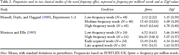
Frequencies used in two classical studies of the word frequency effect, expressed as frequency per million words and as Zipf values

Study Condition fpmw Zipf

Monsell, Doyle, and Haggard (1989), Experiments 1–2 Low-frequency words (N = 48) 2.12 (2.22) 3.15 (0.39)

Medium-frequency words (N = 48) 15.40 (10.81) 4.09 (0.29)

High-frequency words (N = 48) 84.65 (62.66) 4.78 (0.40)

Morrison and Ellis (1995) Low-frequency words (N = 24) 6.52 (4.61) 3.66 (0.44)

High-frequency words (N = 24) 166.03 (168.4) 5.07 (0.37)

Early-acquired words (N = 24) 33.49 (34.8) 4.34 (0.44)

Late-acquired words (N = 24) 9.91 (16.5) 3.63 (0.55)

Note: Means, with standard deviations in parentheses. Frequencies based on SUBTLEX-UK. fpmw = frequency per million words.

Contextual diversity

Adelman, Brown, and Quesada (2006; see also Adelman & Brown, 2008; Perea, Soares, & Comesaña, 2013; Yap, Tan, Pexman, & Hargreaves, 2011) argued that not so much the frequency of occurrence of a word matters, but the number of contexts in which the word appears. Words only encountered in a small number of contexts (say, a word with a frequency of 100 occurring in one or two television episodes) will be more difficult to process than equally frequent words encountered in a variety of contexts (e.g., a word with a frequency count of 100 used in 80 different broadcasts). A good proxy for contextual diversity (CD) is the number of television programmes/films (or the percentage of programmes/films) in which the word appears. Brysbaert and New (2009) indeed observed that log(CD) explained up to 4% of variance more in lexical decision times than log(frequency). Part of the advantage was methodological, however. Two factors were involved. First, the effect of log(CD) on reaction times (RTs) is more linear than the effect of log(frequency), which becomes flat for high-frequency words, as can be seen in Figure 1. When nonlinear regression analysis was used, the difference between CD and frequency became smaller than 2%. Another part of the difference was due to the fact that some words occurred with very high frequency in a few films because they were the names of main characters (e.g., archer, bay, brown). The CD statistic is less influenced by these instances than the frequency statistic.

Still, the CD measure seems to have added value. Therefore, we provide this information for the different corpora we used (full corpus, CBeebies, CBBC). The values are available both as the total number of television programmes in which the word occurred and as the percentage of television programmes in which the word was encountered. As indicated above, the total number of broadcasts in the complete corpus was 45,099. The number of broadcasts in CBeebies was 4847; in CBBC it was 4848.⁴

Part-of-Speech dependent frequencies

For many purposes it is good to know what roles words play in sentences and the relative frequencies of these roles (Brysbaert, New, & Keuleers, 2012). This enables researchers interested in nouns, for instance, to limit their stimulus materials to words that are always (or mostly) used as nouns. It also allows researchers to know whether an inflected word is used more often as an adjective (e.g., appalling) or as a verb (e.g., played). This is important information to decide which words to include in rating studies (e.g., Kuperman, Stadthagen-Gonzalez, & Brysbaert, 2012).

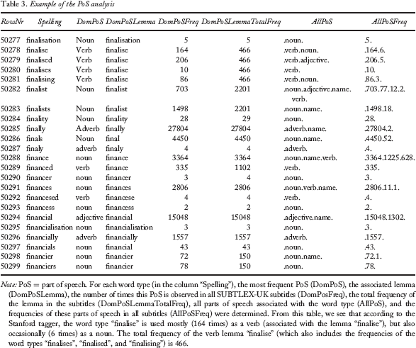
Part-of-Speech (PoS) frequencies can only be obtained after the corpus has been parsed (i.e., the sentences broken down into their constituent parts) and tagged (i.e., the words given their correct part of speech in the sentence). For a long time this was virtually impossible given the amount of work involved. However, the development of automatic PoS taggers has made it possible to get a reasonably good (though not perfect) outcome in reasonable time and at an affordable price. For a long time, the CLAWS tagger developed at the University of Lancaster was the golden standard (Garside & Smith, 1997; Lancaster University Centre for Computer Corpus Research on Language, n.d.). It was used for the BNC corpus, and we also used it for our SUBTLEX-US corpus (Brysbaert et al., 2012). However, in recent years the Stanford tagger (initial version: Toutanova, Klein, Manning, & Singer, 2003; The Stanford Natural Language Processing Group, n.d.) has become a worthy competitor. As it happens, the outcome of the first analyses with the Stanford tagger correlated more with the BLP word processing times than the outcome of the CLAWS tagger did. As indicated in Footnote 3, this was due to the fact that the Stanford tagger is more consistent in dehyphenating words than CLAWS. When the subtitles were cleared of hyphens before running the taggers, both gave comparable output.

Another advantage of the Stanford software⁵ is that it gives the most likely lemma associated with an inflected form. The lemmatization is based on an algorithm developed by Minnen, Carroll, and Pearce (2001). It works on two main principles. First, it looks up whether a word form is present in the dictionary. If so, then the associated lemma can be read out. If a word is lacking, the most likely lemma is allocated on the basis of rules and pattern comparisons (e.g., the most likely lemma of the stimulus “martialisations”, identified as a noun, is “martialisation”; and the most likely lemma of the stimulus “Martialis”, identified as a name, is “Martialis”). As discussed at greater length in Brysbaert et al. (2012), the outcome of these algorithms is not 100% correct⁶ and, hence, should always be checked by the user, certainly for low-frequency words. However, they are a big step forward (with accuracy estimates of 97% and higher) and, therefore, are provided in our database. More precisely, we give information about the most frequent PoS associated with each word type, the frequency of this PoS, and the lemma associated with it, next to all the parts of speech associated with the word type and their respective frequencies. Because of the lemmatization and because the output was as good as that of CLAWS, the data presented in the SUBTLEX-UK database are based on the Stanford parser and tagger. Table 3 gives an example of the output. All frequencies are given as raw frequency counts based on the entire corpus, because this value is the most informative to calculate derived statistics from (e.g., the percentage use as the dominant PoS).
Table 3.
Example of the PoS analysis

RowNr Spelling DomPoS DomPoSLemma DomPoSFreq DomPoSLemmaTotalFreq AllPoS AllPoSFreq

50277 finalisation Noun finalisation 5 5 .noun. .5.

50278 finalise Verb finalise 164 466 .verb.noun. .164.6.

50279 finalised Verb finalise 206 466 .verb.adjective. .206.5.

50280 finalises Verb finalise 10 466 .verb. .10.

50281 finalising Verb finalise 86 466 .verb.noun. .86.3.

50282 finalist Noun finalist 703 2201 .noun.adjective.name.verb. .703.77.12.2.

50283 finalists Noun finalist 1498 2201 .noun.name. .1498.18.

50284 finality Noun finality 28 29 .noun. .28.

50285 finally Adverb finally 27804 27804 .adverb.name. .27804.2.

50286 finals Noun final 4450 4450 .noun.name. .4450.52.

50287 finaly adverb finaly 4 4 .adverb. .4.

50288 finance noun finance 3364 3364 .noun.name.verb. .3364.1225.628.

50289 financed verb finance 335 1102 .verb. .335.

50290 financer noun financer 3 4 .noun. .3.

50291 finances noun finances 2806 2806 .noun.verb.name. .2806.11.1.

50292 financesed verb financese 4 4 .verb. .4.

50293 financess noun financess 2 2 .noun. .2.

50294 financial adjective financial 15048 15048 .adjective.name. .15048.1302.

50295 financialisation noun financialisation 3 3 .noun. .3.

50296 financially adverb financially 1557 1557 .adverb. .1557.

50297 financials noun financial 43 43 .noun. .43.

50298 financier noun financier 72 150 .noun.name. .72.1.

50299 financiers noun financier 78 150 .noun. .78.

Note: PoS = part of speech. For each word type (in the column “Spelling”), the most frequent PoS (DomPoS), the associated lemma (DomPoSLemma), the number of times this PoS is observed in all SUBTLEX-UK subtitles (DomPosFreq), the total frequency of the lemma in the subtitles (DomPoSLemmaTotalFreq), all parts of speech associated with the word type (AllPoS), and the frequencies of these parts of speech in all subtitles (AllPoSFreq) were determined. From this table, we see that according to the Stanford tagger, the word type “finalise” is used mostly (164 times) as a verb (associated with the lemma “finalise”), but also occasionally (6 times) as a noun. The total frequency of the verb lemma “finalise” (which also includes the frequencies of the word types “finalises”, “finalised”, and “finalising”) is 466.

Bigram frequencies

Because extra information can be obtained from word combinations (Arnon & Snider, 2010; Baayen, Milin, Filipovic Durdevic, Hendrix, & Marelli, 2011; Siyanova-Chanturia, Conklin, & van Heuven, 2011), we also collected word bigram frequencies in the entire corpus (i.e., the frequency with which word pairs were observed). This resulted in over 1.5 million lines of consecutive word pairs observed in the corpus. For each pair we give information about the number of times it was observed, the symbols written between the words (space, punctuation mark, hyphen, …) and their respective frequencies. This makes it possible for everyone to calculate interesting additional metrics. For instance, it allowed us to add the 787 hyphenated words with a frequency count of more than 100 (fpwm = 0.5) to the database.⁷ It also allowed us to warn researchers when a compound word is more likely to be written as two separate words than as a single word (for instance, the word “makeup” is observed 308 times in the subtitles (Zipf = 3.18), but the spellings “make-up” and “make up” have a combined frequency of 8998, making “makeup” a bad choice for a low-frequency word).

Correlations with Lexical Decision Measures

Given the ease with which word frequencies can be collected nowadays, it is important to check whether a new frequency measure adds something extra to the existing ones. On the basis of previous research, we can expect this to be the case given the superiority of subtitle-based frequency estimates, but still it is good to test this explicitly, also to make sure no calculation errors have been made. The most interesting dataset is the BLP (Keuleers et al., 2012), which provides lexical decision reaction times and accuracy measures of British students for over 28 thousand monosyllabic and disyllabic words. The main competitors to the SUBTLEX-UK word frequencies are the BNC frequencies, the CELEX frequencies, and the SUBTLEX-US frequencies. Words not observed in a corpus were assigned a frequency of 0, and log frequencies were the Zipf values (with Laplace transformation). The Laplace transformation was also used for the CD measure.

Table 4 shows the results for the accuracy data. As expected, the SUBTLEX-UK frequencies outperform the other measures, more so for the CD measure than for the Zipf measure. Because of the large number of observations, the differences are all highly significant. For instance, the t-value of the Hotelling–Williams test (Steiger, 1980)⁸ of the difference in correlation with SUBTLEX-UK (Zipf) and BNC (Zipf) equals 16.8 (df = 28,282, p < .001). In terms of percentage variance explained, the difference is nearly 3%, which is high given that many variables explain less than 1% of variance, once the effects of word frequency, word length, and similarity to other words are partialled out (Brysbaert, Buchmeier, et al., 2011; Brysbaert & Cortese, 2011; Kuperman et al., 2012).
Table 4.
Correlations between the various frequency measures and the BLP accuracy data

Frequency measure SUBTLEX-UK SUBTLEX-UK_CD SUBTLEX-US BNC Celex CBeebies CBBC

Accuracy .600 .628 .557 .564 .553 .390 .535

SUBTLEX-UK .992 .881 .898 .858 .724 .887

SUBTLEX-UK_CD .877 .904 .866 .702 .876

SUBTLEX-US .830 .830 .705 .851

BNC .927 .633 .789

Celex .642 .778

CBeebies .821

Percentage of variance accounted for

SUBTLEX-UK (Zipf) 40.4

SUBTLEX-UK [log(CD + 1)] 47.1

SUBTLEX-US (Zipf) 35.7

BNC (Zipf) 35.9

Celex (Zipf) 34.6

Note: The upper part shows the correlations. The lower part shows the percentages of variance accounted for by nonlinear regression analyses (lm-procedure in R, restricted cubic splines with 4 knots). BLP = British Lexicon Project; BNC = British National Corpus; CD = contextual diversity. N = 28,285.

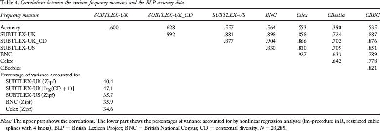
Interestingly, the correlations with the childhood frequencies are much lower, in particular the correlation with the CBeebies frequencies (preschool children). Two reasons for this are the smaller sizes of the corpora (including the many missing words not known to children but given rather high Zipf estimates) and the fact that the overall SUBTLEX-UK frequencies include the subtitles from CBeebies and CBBC television programmes (almost 10% of the total SUBTLEX-UK).

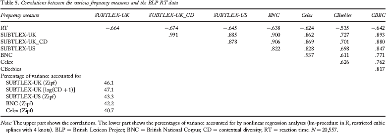
Table 5 shows the correlations for the reaction times (RTs) to the words. Because RTs are only interesting when the words are known, we set percentage accuracy to >66% (N = 20,557). Very much the same picture appears, with superior performance for the SUBTLEX-UK measures (CD slightly more so than Zipf).
Table 5.
Correlations between the various frequency measures and the BLP RT data

Frequency measure SUBTLEX-UK SUBTLEX-UK_CD SUBTLEX-US BNC Celex CBeebies CBBC

RT −.664 −.674 −.645 −.638 −.624 −.535 −.642

SUBTLEX-UK .991 .885 .900 .862 .727 .893

SUBTLEX-UK_CD .878 .906 .869 .701 .880

SUBTLEX-US .822 .828 .698 .847

BNC .937 .611 .771

Celex .626 .762

CBeebies .817

Percentage of variance accounted for

SUBTLEX-UK (Zipf) 46.1

SUBTLEX-UK [log(CD + 1)] 47.1

SUBTLEX-US (Zipf) 43.3

BNC (Zipf) 42.2

Celex (Zipf) 40.7

Note: The upper part shows the correlations. The lower part shows the percentages of variance accounted for by nonlinear regression analyses (lm-procedure in R, restricted cubic splines with 4 knots). BLP = British Lexicon Project; BNC = British National Corpus; CD = contextual diversity; RT = reaction time. N = 20,557.

To make sure that the higher correlations between SUBTLEX-UK and the BLP measures than between SUBTLEX-US and BLP were due to language congruency and not to the better quality of SUBTLEX-UK overall, we ran similar analyses of the ELP data, which were collected on American students. As can be seen in Table 6, the difference between SUBTLEX-UK and SUBTLEX-US indeed has to do with differences in word use between the two languages rather than with the inherent qualities of the frequency lists. Whereas the SUBTLEX-UK frequencies are better for the British BLP data (see Tables 4 and 5), the SUBTLEX-US data are better for the American ELP data (Table 6).
Table 6.
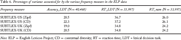
Percentages of variance accounted for by the various frequency measure in the ELP data

Frequency measure Accuracy_LDT (N = 40,468) RT_LDT (N = 33,997) RT_nam (N = 33,997)

SUBTLEX-US (Zipf) 20.5 36.7 26.0

SUBTLEX-US (CD) 22.3 37.2 26.1

SUBTLEX-UK (Zipf) 19.0 34.8 24.2

SUBTLEX-UK (CD) 20.5 34.8 24.2

Note: ELP = English Lexicon Project; CD = contextual diversity; RT = reaction time; LDT = lexical decision task.

Correlations with the Children's Printed Word Database (CPWD)

The best existing British database of word frequencies for children is the Children's Printed Word Database (CPWD; available at http://www.essex.ac.uk/psychology/cpwd/; checked on May 21, 2013). It includes the frequencies with which 12,193 different word types are observed in 1011 books (995,927 tokens) for 5–9-year-old children in the UK (Masterson, Stuart, Dixon, & Lovejoy, 2010). We could download data for 9659 word types from the database, 9125 of which were also in the SUBTLEX-UK list (the ones not in the list were mainly genitive forms, hyphenated forms, and numbers). Table 7 gives the correlations between log CPWD frequencies and various SUBTLEX-UK frequencies for the 9125 shared word types. As can be seen, the correlations are reasonably high, in particular with the CBeebies word frequencies. The Hotelling–Williams test indicated significant differences between the CBeebies frequencies and the other frequencies (e.g., difference between CBeebies and CBBC, t(9122) = 15.6, p < .001). This confirms that the SUBTLEX-UK children frequencies are an interesting addition to the CPWD frequencies and can be used to study frequency trajectories from childhood to adulthood⁹ (Lété & Bonin, 2013).
Table 7.
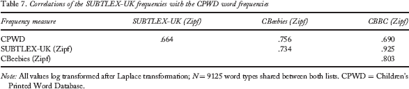
Correlations of the SUBTLEX-UK frequencies with the CPWD word frequencies

Frequency measure SUBTLEX-UK (Zipf) CBeebies (Zipf) CBBC (Zipf)

CPWD .664 .756 .690

SUBTLEX-UK (Zipf) .734 .925

CBeebies (Zipf) .803

Note: All values log transformed after Laplace transformation; N = 9125 word types shared between both lists. CPWD = Children's Printed Word Database.

Discussion

In this paper, we presented a new database of word frequencies for British English, based on television subtitles. On the basis of our previous research, we expected that these frequencies would better predict word processing performance than word frequencies based on written sources (in particular, the British National Corpus). This indeed turned out to be the case, when we tried to predict the lexical decision times and accuracies of the British Lexicon Project (Tables 4 and 5). The British subtitle frequencies were also better for predicting the BLP data than were the American subtitle frequencies, but they were inferior for accounting for the ELP data, in line with the observation that word usage is not completely the same in British and American English. The extra variance accounted for amounted to 3–5%, which is considerable given that many variables explain less than 1% of the variance once the effects of word frequency, length, and similarity to other words are partialled out (Brysbaert, Buchmeier, et al., 2011; Brysbaert & Cortese, 2011; Kuperman et al., 2012).

While analysing the findings, we were once again struck by how misleading the standardized word frequency measure fpmw (frequency per million words) is to understand the word frequency effect. Therefore, we proposed an alternative, the Zipf scale, which is better suited to the use of word frequencies in psychological research. This scale goes from slightly less than 1 to slightly more than 7 and can easily be interpreted as follows: Values of 3 and less are low-frequency words; values of 4 or more are high-frequency words. Words not in SUBTLEX-UK get a Zipf value of 0.696 when the frequencies are based on the complete corpus, 1.864 when the CBBC frequencies are used, and 2.231 when the CBeebies frequencies are used. The differences in minimal values are caused by the differences in corpus size and agree with the fact that missing words of interest in CBeebies or CBBC are likely to be more familiar than words not found in the entire corpus.

In addition to the word frequencies, the new database offers other information, which will allow British researchers to do cutting-edge investigations. These are:
Part-of-speech-related frequencies, which make it possible for researchers to better control their stimulus materials.

A measure of contextual diversity (CD), which is particularly interesting for predicting which words will be known and which not (compare Tables 4 and 5).

Word frequencies in materials aimed at very young (preschool) and young (primary school) children.

Information about word bigrams.

Availability

The SUBTLEX-UK data are available in three easy-to-use files. The first one (SUBTLEX-UK_all) is a 332,988 × 15 matrix containing information of all word types (including numbers) encountered in the dehyphenated subtitles. The 15 columns give information about:
The spelling of the word type (Spelling).

The number of times the word has been counted in all subtitles (Freq).

The number of times the word started with a capital (CapitFreq).

The percentage of broadcasts containing the word type in all subtitles (CD).

The number of broadcasts containing the word in all subtitles (CDCount).

The most frequent part of speech of the word (DomPoS).

The number of times this dominant Pos was observed (DomPosFreq).

The lemma associated with the dominant Pos (DomPosLemma).

The number of times this lemma was observed in all subtitles (DomPosLemmaFreq).

The summed frequencies of all the times this lemma was observed irrespective of the PoS (DomPosLemmaTotalFreq).

All parts of speech taken by the word type (AllPos).

The respective frequencies of these PoS (AllPosFreq).

The associated lemma information (AllLemmaPos, AllLemmaPosFreq, AllLemma PosTotalFreq).

The second file (SUBTLEX-UK) contains more information about the 160,022 word types (159,235 single words and 787 hyphenated words) that are observed in more than one broadcast and which only contain letter information (i.e., no digits or nonalphanumerical symbols). This file is the file most psycholinguistic researchers will want to use. It has 27 columns, containing:
The word type.

The frequency counts in all subtitles, the CBeebies subtitles, the CBBC subtitles, and the British National corpus.

The Zipf values associated with the various frequencies.

The CD counts and percentages in the three SUBTLEX corpora.

The dominant PoS, its associated lemma, and their frequencies.

All the PoS and frequencies of the word.

The frequency of the word starting with a capital.

Whether the lower-case spelling of the word type was accepted by a UK word spell checker (UK), a US word spell checker (US), both spell checkers (UK US), or none (X)¹⁰. This is an interesting column when words must be selected, and one wants to avoid the inclusion of names or other uninteresting entries.

Whether the entry contains a hyphen (cf. the 787 added entries with hyphens).

Whether the entry has another homophonic entry. This is interesting for finding homophones, but also to make sure selected low-frequency words do not have a higher frequency spelling alternative.

Whether or not the word type has been encountered as a bigram in the subtitles.

The frequency of the bigram (summed across all types of intervening symbols, in particular, blank spaces, punctuation marks, and hyphens).

Finally, the third file (SUBTLEX-UK_bigrams) contains information about word pairs. Because this file has nearly 2 million lines of information, it cannot be made available as an Excel file (although we have such a file with all entries observed 12 times or more). Each line contains information about Word 1 and Word 2, the frequency of the combination, the CD count of the combination, and which symbols were found between the two words with which frequencies. This is important information when researchers want to include transition probabilities in their investigations, or when expressions (e.g., object names, particle verbs) consist of two words.

Zipf value	fpmw	Examples
1	0.01	antifungal, bioengineering, farsighted, harelip, proofread
2	0.1	airstream, doorkeeper, neckwear, outsized, sunshade
3	1	beanstalk, cornerstone, dumpling, insatiable, perpetrator
4	10	dirt, fantasy, muffin, offensive, transition, widespread
5	100	basically, bedroom, drive, issues, period, spot, worse
6	1000	day, great, other, should, something, work, years
7	10,000	and, for, have, I, on, the, this, that, you

Study	Condition	fpmw	Zipf
Monsell, Doyle, and Haggard (1989), Experiments 1–2	Low-frequency words (N = 48)	2.12 (2.22)	3.15 (0.39)
	Medium-frequency words (N = 48)	15.40 (10.81)	4.09 (0.29)
	High-frequency words (N = 48)	84.65 (62.66)	4.78 (0.40)
Morrison and Ellis (1995)	Low-frequency words (N = 24)	6.52 (4.61)	3.66 (0.44)
	High-frequency words (N = 24)	166.03 (168.4)	5.07 (0.37)
	Early-acquired words (N = 24)	33.49 (34.8)	4.34 (0.44)
	Late-acquired words (N = 24)	9.91 (16.5)	3.63 (0.55)

RowNr	Spelling	DomPoS	DomPoSLemma	DomPoSFreq	DomPoSLemmaTotalFreq	AllPoS	AllPoSFreq
50277	finalisation	Noun	finalisation	5	5	.noun.	.5.
50278	finalise	Verb	finalise	164	466	.verb.noun.	.164.6.
50279	finalised	Verb	finalise	206	466	.verb.adjective.	.206.5.
50280	finalises	Verb	finalise	10	466	.verb.	.10.
50281	finalising	Verb	finalise	86	466	.verb.noun.	.86.3.
50282	finalist	Noun	finalist	703	2201	.noun.adjective.name.verb.	.703.77.12.2.
50283	finalists	Noun	finalist	1498	2201	.noun.name.	.1498.18.
50284	finality	Noun	finality	28	29	.noun.	.28.
50285	finally	Adverb	finally	27804	27804	.adverb.name.	.27804.2.
50286	finals	Noun	final	4450	4450	.noun.name.	.4450.52.
50287	finaly	adverb	finaly	4	4	.adverb.	.4.
50288	finance	noun	finance	3364	3364	.noun.name.verb.	.3364.1225.628.
50289	financed	verb	finance	335	1102	.verb.	.335.
50290	financer	noun	financer	3	4	.noun.	.3.
50291	finances	noun	finances	2806	2806	.noun.verb.name.	.2806.11.1.
50292	financesed	verb	financese	4	4	.verb.	.4.
50293	financess	noun	financess	2	2	.noun.	.2.
50294	financial	adjective	financial	15048	15048	.adjective.name.	.15048.1302.
50295	financialisation	noun	financialisation	3	3	.noun.	.3.
50296	financially	adverb	financially	1557	1557	.adverb.	.1557.
50297	financials	noun	financial	43	43	.noun.	.43.
50298	financier	noun	financier	72	150	.noun.name.	.72.1.
50299	financiers	noun	financier	78	150	.noun.	.78.

Frequency measure	Accuracy_LDT (N = 40,468)	RT_LDT (N = 33,997)	RT_nam (N = 33,997)
SUBTLEX-US (Zipf)	20.5	36.7	26.0
SUBTLEX-US (CD)	22.3	37.2	26.1
SUBTLEX-UK (Zipf)	19.0	34.8	24.2
SUBTLEX-UK (CD)	20.5	34.8	24.2

Frequency measure	SUBTLEX-UK (Zipf)	CBeebies (Zipf)	CBBC (Zipf)
CPWD	.664	.756	.690
SUBTLEX-UK (Zipf)		.734	.925
CBeebies (Zipf)			.803

Footnotes

1

On the basis of anecdotal evidence we can add that these subtitles are also appreciated by viewers with English as second language.

2

Brysbaert and New (2009) reported that the word type frequencies themselves show little difference once the corpus contains 30 million words, a finding that was replicated in the present analyses.

3

Dehyphenation also occurs in automatic text parsers, such as CLAWS and the Stanford parser (to be described later). Because the Stanford parser dehyphenates more words than CLAWS, the outcome of this parser outperformed that of CLAWS on the raw corpus, but no longer on the dehyphenated corpus.

4

The reason why these numbers are very similar is that both channels have a similar rotation of programmes with repeats after a rather short period of time.

5

A disadvantage of the Stanford tagger is that in its default mode it Americanizes the spellings of the words. So, one must be careful to change this when one is working with British spellings.

6

A notorious example is “horsefly”, which both CLAWS and Stanford parse as an adverb (arguably because the word is not in the programme's lexicon, so that too much reliance is put on the end letters –ly). Ironically, Stanford does correctly classify “horseflies” as a noun associated with the lemma “horsefly” (presumably because the end letters, –lies, are more likely to be associated with plural nouns than with other parts of speech).

7

These frequencies were not subtracted from the frequencies of the individual words, under the assumption that the component words of a hyphenated word get coactivated upon seeing the hyphenated word.

8

An easy introduction to the test and an Excel file to calculate the exact values are available on the website ()

9

SUBTLEX-UK frequencies not including childhood frequencies can easily be obtained by subtracting the CBeebies and CBBC frequency counts from the total frequency counts.

10

The speller was the MS Office 2007 spellchecker, augmented with a list of lemmas one of the authors (M.B.) is compiling.

References

Adelman

J. S.

, & Brown

G. D.

(2008). Modeling lexical decision: The form of frequency and diversity effects. Psychological Review, 115(1), 214–227. doi: 10.1037/0033-295X.115.1.214

Adelman

J. S.

, Brown

G. D. A.

, & Quesada

J. F.

(2006). Contextual diversity, not word frequency, determines word naming and lexical decision times. Psychological Science, 17, 814–823. doi: 10.1111/j.1467-9280.2006.01787.x

Arnon

, & Snider

(2010). More than words: Frequency effects for multi-word phrases. Journal of Memory and Language, 62(1), 67–82. doi: 10.1016/j.jml.2009.09.005

Baayen

R. H.

, Milin

, Filipovic Durdevic

, Hendrix

, & Marelli

(2011). An amorphous model for morphological processing in visual comprehension based on naive discriminative learning. Psychological Review, 118, 438–481. doi: 10.1037/a0023851

Baayen

R. H.

, Piepenbrock

, & Gulikers

(1995). The CELEX lexical database [CD-ROM]. Philadelphia: University of Pennsylvania, Linguistic Data Consortium.

Balota

D. A.

, Yap

M. J.

, Cortese

M. J.

, Hutchison

K. A.

, Kessler

, Loftis

, … Treiman

(2007). The English Lexicon project. Behavior Research Methods, 39, 445–459. doi: 10.3758/BF03193014

Brysbaert

, Buchmeier

, Conrad

, Jacobs

A. M.

, Bölte

, & Böhl

(2011). The word frequency effect: A review of recent developments and implications for the choice of frequency estimates in German. Experimental Psychology, 58, 412–424. doi: 10.1027/1618-3169/a000123

Brysbaert

, & Cortese

M. J.

(2011). Do the effects of subjective frequency and age of acquisition survive better word frequency norms? Quarterly Journal of Experimental Psychology, 64, 545–559. doi: 10.1080/17470218.2010.503374

Brysbaert

, & Diependaele

(2013). Dealing with zero word frequencies: A review of the existing rules of thumb and a suggestion for an evidence-based choice. Behavior Research Methods, 45, 422–430. doi: 10.3758/s13428-012-0270-5

10.

Brysbaert

, Keuleers

, & New

(2011). Assessing the usefulness of google books’ word frequencies for psycholinguistic research on word processing. Frontiers in Psychology, 2, 27. doi: 10.3389/fpsyg.2011.00027

11.

Brysbaert

, & New

(2009). Moving beyond Kucera and Francis: A critical evaluation of current word frequency norms and the introduction of a new and improved word frequency measure for American English. Behavior Research Methods, 41, 977–990. doi: 10.3758/BRM.41.4.977

12.

Brysbaert

, New

, & Keuleers

(2012). Adding part-of-speech information to the SUBTLEX-US word frequencies. Behavior Research Methods, 44, 991–997. doi: 10.3758/s13428-012-0190-4

13.

Cai

, & Brysbaert

(2010). SUBTLEX-CH: Chinese word and character frequencies based on film subtitles. PLOS ONE, 5, e10729. doi: 10.1371/journal.pone.0010729

14.

Children's Printed Word Database. Database of printed word frequencies as read by children aged between 5 & 9. Retrieved May 21, 2013, from http://www.essex.ac.uk/psychology/cpwd/

15.

Cuetos

, Glez-Nosti

, Barbon

, & Brysbaert

(2011). SUBTLEX-ESP: Spanish word frequencies based on film subtitles. Psicologica, 32, 133–143.

16.

Dimitropoulou

, Duñabeitia

J. A.

, Avilés

, Corral

, & Carreiras

(2010). Subtitle-based word frequencies as the best estimate of reading behavior: The case of Greek. Frontiers in Psychology, 1(218), 1–12.

17.

Ferrand

, New

, Brysbaert

, Keuleers

, Bonin

, Meot

, … Pallier

(2010). The french lexicon project: Lexical decision data for 38,840 french words and 38,840 pseudowords. Behavior Research Methods, 42, 488–496. doi: 10.3758/BRM.42.2.488

18.

Garside, R., & Smith, N. (1997). A hybrid grammatical tagger: CLAWS4. In R. Garside, G. Leech, & A. McEnery (Eds.), Corpus annotation: Linguistic information from computer text corpora (pp. 102–121). London: Longman

19.

Government United Kingdom (1988). Copyright, Designs and Patents Act 1988. Retrieved from http://www.legislation.gov.uk/ukpga/1988/48/contents

20.

Keuleers

, Brysbaert

, & New

(2010). SUBTLEX-NL: A new frequency measure for Dutch words based on film subtitles. Behavior Research Methods, 42, 643–650. doi: 10.3758/BRM.42.3.643

21.

Keuleers

, Lacey

, Rastle

, & Brysbaert

(2012). The British Lexicon Project: Lexical decision data for 28,730 monosyllabic and disyllabic English words. Behavior Research Methods, 44, 287–304. doi: 10.3758/s13428-011-0118-4

22.

Kilgarriff, A. (2006). BNC database and word frequency lists. Retrieved May 13, 2013, from http://www.kilgarriff.co.uk/bnc-readme.html

23.

Kučera

, & Francis

(1967). Computational analysis of present-day American English. Providence, RI: Brown University Press.

24.

Kuperman

, & Bertram

(2013). Moving spaces: Spelling alternation in english noun-noun compounds. Language and Cognitive Processes, 28, 939–966.

25.

Kuperman

, Stadthagen-Gonzalez

, & Brysbaert

(2012). Age-of-acquisition ratings for 30 thousand english words. Behavior Research Methods, 44, 978–990. doi: 10.3758/s13428-012-0210-4

26.

Lancaster University Centre for Computer Corpus Research on Language (n.d.). CLAWS part-of-speech tagger for English. Retrieved May 17, 2013, from http://ucrel.lancs.ac.uk/claws/

27.

Lété

, & Bonin

(2013). Does frequency trajectory influence word identification? A cross-task comparison. The Quarterly Journal of Experimental Psychology, 66(5), 973–1000. doi: 10.1080/17470218.2012.723725

28.

Masterson

, Stuart

, Dixon

, & Lovejoy

(2010). Children's printed word database: Continuities and changes over time in children's early reading vocabulary. British Journal of Psychology, 101(2), 221–242. doi: 10.1348/000712608X371744

29.

Minnen

, Carroll

, & Pearce

(2001). Applied morphological processing of English. Natural Language Engineering, 7(3), 207–223. doi: 10.1017/S1351324901002728

30.

Monsell

, Doyle

M. C.

, & Haggard

P. N.

(1989). Effects of frequency on visual word recognition tasks – Where are they? Journal of Experimental Psychology: General, 118, 43–71. doi: 10.1037/0096-3445.118.1.43

31.

Morrison

C. M.

, & Ellis

A. W.

(1995). Roles of word frequency and age of acquisition in word naming and lexical decision. Journal of Experimental Psychology. Learning, Memory, and Cognition, 21(1), 116–133. doi: 10.1037/0278-7393.21.1.116

32.

New

, Brysbaert

, Veronis

, & Pallier

(2007). The use of film subtitles to estimate word frequencies. Applied Psycholinguistics, 28, 661–677. doi: 10.1017/S014271640707035X

33.

Perea

, Soares

A. P.

, & Comesaña

(2013). Contextual diversity is a main determinant of word identification times in young readers. Journal of Experimental Child Psychology, 116, 37–44. doi: 10.1016/j.jecp.2012.10.014

34.

Siyanova-Chanturia

, Conklin

, & van Heuven

W. J. B.

(2011). Seeing a phrase “time and again” matters: The role of phrasal frequency in the processing of multiword sequences. Journal of Experimental Psychology-Learning Memory and Cognition, 37(3), 776–784. doi: 10.1037/a0022531

35.

Steiger

J. H.

(1980). Tests for comparing elements of a correlation matrix. Psychological Bulletin, 87, 245–251. doi: 10.1037/0033-2909.87.2.245

36.

The Stanford Natural Language Processing Group (n.d.). Stanford Log-linear Part-Of-Speech Tagger. Retrieved May 17, 2013, from http://nlp.stanford.edu/downloads/tagger.shtml

37.

Toutanova

, Klein

, Manning

C. D.

, & Singer

(2003). Feature-rich part-of-speech tagging with a cyclic dependency network. In Proceedings of the 2003 conference of the North American chapter of the association for computational linguistics on human language technology-volume 1 (pp. 173–180). Association for Computational Linguistics.

38.

Yap

M. J.

, Tan

S. E.

, Pexman

P. M.

, & Hargreaves

I. S.

(2011). Is more always better? Effects of semantic richness on lexical decision, speeded pronunciation, and semantic classification. Psychonomic Bulletin & Review, 18(4), 742–750. doi: 10.3758/s13423-011-0092-y

39.

Zipf

G. K.

(1949). Human behavior and the principle of least effort. Cambridge, MA: Addison-Wesley.

Frequency measure	SUBTLEX-UK	SUBTLEX-UK_CD	SUBTLEX-US	BNC	Celex	CBeebies	CBBC
Accuracy	.600	.628	.557	.564	.553	.390	.535
SUBTLEX-UK		.992	.881	.898	.858	.724	.887
SUBTLEX-UK_CD			.877	.904	.866	.702	.876
SUBTLEX-US				.830	.830	.705	.851
BNC					.927	.633	.789
Celex						.642	.778
CBeebies							.821
Percentage of variance accounted for
SUBTLEX-UK (Zipf)	40.4
SUBTLEX-UK [log(CD + 1)]	47.1
SUBTLEX-US (Zipf)	35.7
BNC (Zipf)	35.9
Celex (Zipf)	34.6

Frequency measure	SUBTLEX-UK	SUBTLEX-UK_CD	SUBTLEX-US	BNC	Celex	CBeebies	CBBC
RT	−.664	−.674	−.645	−.638	−.624	−.535	−.642
SUBTLEX-UK		.991	.885	.900	.862	.727	.893
SUBTLEX-UK_CD			.878	.906	.869	.701	.880
SUBTLEX-US				.822	.828	.698	.847
BNC					.937	.611	.771
Celex						.626	.762
CBeebies							.817
Percentage of variance accounted for
SUBTLEX-UK (Zipf)	46.1
SUBTLEX-UK [log(CD + 1)]	47.1
SUBTLEX-US (Zipf)	43.3
BNC (Zipf)	42.2
Celex (Zipf)	40.7

Subtlex-UK: A New and Improved Word Frequency Database for British English

Abstract

Keywords

Method

Corpus collection

Text cleaning

Word Frequency Measures

Word frequency counts

A standardized frequency measure: The Zipf scale

Contextual diversity

Part-of-Speech dependent frequencies

Bigram frequencies

Correlations with Lexical Decision Measures

Correlations with the Children's Printed Word Database (CPWD)

Discussion

Availability

Footnotes

1

2

3

4

5

6

7

8

9

10

References