Comparison of Petri Net and Finite State Machine Discrete Event Control of Distributed Surveillance Network

Abstract

Wireless sensor networks are an important military technology with civil and scientific applications. In this article, we derive a discrete event controller system for distributed surveillance networks that consists of three interacting hierarchies—sensing, communications, and command. Petri Net representations of the hierarchies provide plant models of resource contention and internal consistency. Control specifications are derived that enforce consistency across the hierarchies. Three controllers are created using different methodologies to satisfy these specifications. The methods used are Petri Net, finite state automata using the Ramadge and Wonham approach, and vector addition control using the Wonham and Li approach. We use the controllers derived to contrast the design methodologies. Our results find these three approaches to be roughly equivalent. Each method has advantages and disadvantages.

1. Introduction

In this article, we derive models of, and controllers for, distributed sensor networks (DSN) consisting of multiple cooperating nodes. Each battery-powered node has wireless communications, local processing, sensor inputs, data storage, and limited mobility. An individual node would be capable of isolated operation, but practical deployment scenarios require coordination among multiple nodes. We are particularly interested in self-organization technologies for these systems. Network self-configuration is needed for the system to adapt to a changing environment [1]. In this article, we derive hierarchical structures that support user control of the distributed system.

Our model uses discrete event dynamic systems (DEDS) formalisms. DEDS have discrete time and state spaces. They are usually asynchronous and non-deterministic. Many DEDS modeling and control methodologies exist and no dominant paradigm has emerged [2, 18, 19, 22-24]. Generally speaking, the three approaches can be classified into two categories-FSM belongs to traditional finite automata based controller category and Petri Net modeled and VDES belongs to the Petri Net based controller family.

We use Petri Nets to model the plants to be controlled. Our sensor network model has three intertwined hierarchies, which evolve independently [11]. We derive controllers to enforce system consistency constraints across the three hierarchies.

Three equivalent controllers are derived using:

(1)

Petri Net [20, 21],

(2)

vector addition [13] and

(3)

Finite State Machine (FSM) techniques [4]. We compare the controllers in terms of expressiveness and performance.

Innovative use of Karp-Miller trees [3] allows us to derive FSM controllers for the Petri Net plant model.

The remainder of the article is organized as follows. Section 1 gives an introduction to Petri Nets and hierarchical node organization. Section 2 describes the structure of the network hierarchies. We provide control specifications in Section 3. The three controller designs, each illustrated with an example, are detailed in Section 4. Section 5 provides simulation results. Section 6 concludes this article.

1.1. Petri Net

Carl Adam Petri defined Petri Nets as a graphic mathematical model for describing information flow in 1962. This model proved versatile in visualizing and analyzing the behavior of asynchronous, concurrent systems. Later research led to the direct application of Petri Nets in automata theory. The Petri Nets can model the relations between events, resources, and system states particularly well [4].

A Petri Net is a bi-partite graph with two classes of nodes: places and transitions. The number of places and transitions are finite and nonzero. Directed arcs connect nodes. Arcs either connect a transition to a place or a place to a transition. Arcs can have an associated integer weight. DEDS state variables are represented by places. Events are represented by transitions. Places contain tokens. The DEDS state space is defined by the marking of the Petri Net. A marking is a vector expressing the number of tokens in each place. The firing of a transition changes the marking of the Petri Net and the state of the DEDS system. The system is nondeterministic in that any enabled transition can fire.

Mathematically, a Petri Net is represented as the tuple S = (P, T, I, O, u) with P: Finite set of places, T: finite set of transitions, I: finite set of arcs from places to transitions, O: finite set of arcs from transitions to places and u is an integer vector representing the current marking [3]. Safeness is a special issue to be considered. A Petri net is safe if all places contain no more than one token. However, a Petri net is called k-safe or k-bounded if no place contains no more than k tokens. An unbounded Petri net may contain an infinite number of tokens in places and has an infinite number of markings. Conversely, a bounded Petri net is essentially a finite state machine with each node corresponding to every reachable state.

In deriving our controllers, we derive Karp-Miller trees from the Petri Nets [3]. Despite their name, Karp Miller trees are graph structures. They represent all possible markings a Petri Net can reach from a given initial marking and ω is usually used to represent an infinite number of tokens in a place if necessary.

1.2. Hierarchical Model Overview and Terminology

In an effort to thoroughly describe the functionality of a remote, multi-modal, mobile sensing network three issues must be addressed:

Network communication - communications must be maintained with the network.

Collaborative sensing - coordinates sensor data interpretation.

Operational command - assigns resources within the network and controls internal system logistics.

Each hierarchy has three levels:

Root - is the top level of the hierarchy. It coordinates among cluster heads and provides top-level guidance.

Cluster head - coordinates lower level controllers and propagates guidance from the root to lower layers.

Leaf - performs low-level tasks and executes commands coming from the upper layers.

We have identified a number of global consistency issues in the system that requires a controller to constrain the actions taken by the hierarchies. These requirements were captured as control specifications and used to derive the appropriate control structures. Figure 1 shows the relations between the three nodes levels. To make the hierarchy adaptive, a cluster head can control any number of leaves. Similarly, a root node can coordinate an arbitrary number of cluster heads.

Figure 1.

Relationships between three nodes levels.

There are three tiers within the network hierarchy design. This design does not, however, limit the physical network to only three levels. Networks intended to cover a large physical area, or to operate in a highly cluttered environment may require more nodes than can be effectively managed by three tiers. For this reason it is desirable to allow recursion within the hierarchy. Internal nodes are inserted between the root node and cluster heads. Internal nodes are implemented by defining either root or cluster head nodes so that they can be connected recursively. This allows complex structures to arise when required by the mission as shown in Fig. 2.

Figure 2.

Example of a more complex structure.

A given physical node will have a “rank” or “level” in each of the above three hierarchies. It is important to note here that the ranks of a node in each of the three hierarchies are independent of one another. A node occupying the cluster head level in the collaborative sensing hierarchy is allowed to occupy any of the three levels in the other two hierarchies and is not restricted in any fashion. This allows for maximum flexibility in terms of network configuration and also grants the network the ability to configure the sensing clusters dynamically to best process information concerning an individual target event occurrence.

2. Network Hierarchies

2.1. Operational Command

The combined operational command hierarchy demonstrates the interaction between the three node levels. It controls allocation of nodes to surveillance regions. This includes mapping unknown territory and discovering obstacles. It also controls node deployment, and decisions to recall nodes.

The network reconfigures itself as priorities change. Initial node deployments are likely to concentrate nodes in regions:

(1)

where it is assumed enemy traffic will be heavy or

(2)

which are of strategic interest to friendly forces.

Over time the network should find the true traffic flows, which are likely to be different than anticipated. Similarly, the strategies of friendly forces change over time.

The root node signals change in strategy to the cluster heads. The root is charged with managing network resources. It also oversees mapping the region of interest, node assignment, node reallocation, network topology, and network recall. Furthermore, the root provides information about these functions to the end user and distributes user preferences and commands to appropriate subnets. Cluster heads are charged with managing the activities of subnets of leaf nodes and other cluster heads. Cluster head responsibilities include generating topology reports, interpreting commands from the root, calculating resource needs, and monitoring resource availability. A leaf node whose responsibilities encompass only a small subsection of the area covered by the entire network only considers the area it monitors and retains no global information. The leaf node is responsible for the direct interaction with the environment. This is limited to terrain mapping and providing position and status information.

2.2. Network Communications

The network communications hierarchy is implemented to maintain data flow in the presence of environmental interference, jamming, and node loss. Actions the hierarchy controls include adjusting transmission power, frequency hopping schedules, ad-hoc routing, and motion to correct interference.

The Petri Net hierarchy describes a communications protocol between the nodes. Critical messages have associated acknowledgements. To ensure connectivity between nodes and their immediate superiors, all messages pushing information up the hierarchy have matching acknowledgements. If an acknowledgement is not received, retransmission occurs according to the parameters set by the end users. When retransmissions are exhausted, a supervisor may have to be replaced. When communications with their supervisor is severed, the leaf and cluster head nodes immediately enter a promotion cycle. The node waits for an indication that a replacement supervisor has been chosen. If none is received, the node promotes itself to the next level. It broadcasts that it has assumed control of the subnet and overtakes supervisory responsibility. If the previous supervisor rejoins the subnet, it may demote itself.

Lost contact between the root node and the user community is more difficult to address. Upon exhausting retransmissions, the root assumes that contact has been lost and the network is isolated. The first action taken is to broadcast a message throughout the network indicating to the user that root contact has been lost. Each node tries to establish contact with the user community and become the new root. If this fails, the network is put to sleep by a command propagated down the hierarchy. It is left to the user to re-establish contact. While in this quiescent mode the network suspends operations, and responds only to a wake command transmitted by a member of the user community.

2.3. Collaborative Sensing

Coordination of sensor data interpretation is based partly on our existing sensor network implementation, which was tested at 29 Palms Marine Base in November 2001 [26].

Initial processing of sensor information is done by the leaf node. Time series data is preprocessed. A median filter reduces white noise. A low pass filter removes high frequency noise. If the signal is still unusable, it is assumed either that the sensor is broken, or that environmental conditions make it impossible. The node temporarily hibernates to save energy. Each node has multiple sensors and may have multiple sensing modalities. This reduces the node's vulnerability to mechanical failure of the sensors and many types of environmental noise [5].

After filtering, the sensor time series are registered to a common coordinate system and given a time stamp. Subsequently, data association determines which detections refer to the same object. A state vector with inputs from multiple sensing modalities can be used for target classification [7]. Each leaf-node can send either a target state vector or the Closest Point of Approach (CPA) event to the cluster head.

A cluster head is selected dynamically. Cluster heads take care of combining these statistics into meaningful track information. Root nodes coordinate activities among cluster heads and follow tracks traversing the area they survey. In this hierarchy, internal nodes are root nodes. They define the sensing topology, which organizes itself from the bottom up. This topology mimics the flow of targets through the system. It has been suggested that this information can guide future node deployment [8].

Sensing hierarchy topology can be calculated using computational geometry and graph theory. A root node can request topology data from all root nodes, cluster heads, and leaf nodes beneath it. Cluster heads can determine sensor coverage statistics, Voronoi diagrams, breach paths, and covered paths in its region. This data defines the system topology [9].

3. Control Specifications

Given the set of states G and the set of events Σ, the controller disables a subset of Σ as necessary at every state g ∊ G. Control specifications are defined by identifying state and event combinations that lead the system to an undesirable state. Each specification is a constraint on the system and the controller's behavior is defined by the set of constraints. Control of the DSN requires coordination of individual node activities within the constraints of mission goals. Each node has a set of responsibilities and must act according to its capabilities in response.

The controller is needed because the system has multiple command hierarchies. Each hierarchy has its own goals. When conflicts between hierarchies arise, the controller resolves them. We identified sequences of events that lead to undesirable states. Three primary issues were found that can cause undesirable system states:

(1)

Movement of a node conflicting with the needs of another hierarchy;

(2)

Nodes attempting to function in the presence of unrecoverable noise; and

(3)

Retreat commands from the command hierarchy should have precedence over all other commands.

Followings are the abbreviations and the set of constraints the controllers impose on the DSN:

CC - operational command

CS - collaborative sensing

NC - network communication

• When a node is waiting for on-board data fusion, it should be prevented from moving by NC, CC, and CS. Also it should not be promoted by NC or by CS until sensing is complete.

• Hibernation induced by unrecoverable noise or saturated signal in SC should also force the node to hibernate in NC and CC. (And vice versa, for leaf nodes only). Wakeup in CS needs to send wake-up to CC/NC

• While the cluster head is in the process of updating its statistics, its leaves should be prevented from moving by NC, CC, or CS.

• While a cluster head node is receiving statistics from its leaf nodes, it should be prevented from moving by NC, CC, or CS.

• When sensor nodes are in low power mode as determined by NC, or damaged mode as determined by CC, they should be prohibited from any moving for prioritized relocation or occlusion adjustments.

• Retreat in CC should supercede all actions, except the propagation of the retreat command.

• Nodes encountering a target signal in the CS should suspend mapping action in CC until sensing is complete.

• Move commands in CC/NC should be delayed while the node is receiving sensing statistics from lower levels in the hierarchy.

4. Controller Design

Each controller design method enforces constraints in its own way. Vector controllers use state vector comparison to determine the transitions that violate the control specifications. Petri Net controllers use slack variables to disable the same transitions. Moore machines determine which strings of events lead to constraint violations.

Controller design is complicated by the existence of uncontrollable and unobservable transitions. Uncontrollable transitions cannot be disabled. Unobservable transitions cannot be detected. When uncontrollable or unobservable transitions lead to undesirable states, the controller design process requires creating alternative constraints that use only controllable transitions. Ideally, the controller should not unnecessarily constrain the system. A methodology for creating non-restrictive controllers is described in [10].

Control specification is usually specified as: lμ ≤ b. Matrix l has a dimension of N (number of control specifications) xM (number of places in the plant); Vector μ has M components representing the number of tokens in each place of the plant and vector b has N integer components, each element representing the total maximal allowed number of tokens in any combination of places.

4.1. Finite State Machine Controller

Verifying system properties, such as safeness, boundedness, and liveness, is done using the Karp-Miller tree. It represents all possible states of the system [4].

Ramadge and Wonham described supervisory control of the discrete event process using finite state automaton [2]. We generalized their contribution and proposed our own innovations.

All reachable state vectors could be infinite, but Karp Miller tree should be finite. Thus, we introduce the symbol omega (ω) in the Karp-Miller tree to indicate that the token number in the corresponding place is unbounded. A 5-tuple plant ℘ = (Q, Σ, δ, q₀, Q _m ) was obtained from the Karp-Miller tree, where Q: all legal and illegal states; Σ: all transitions; δ: next state function; q₀: initial state; Q _m : only legal states. Because the FSM generated without constraints contains illegal states, we enforce a state feedback map function on the plant to restrict its behavior. Let Γ = (0, 1)^{Σ _c} be a set of control patterns. For each γ ∊ Γ, a control pattern has |Σ _c | bits. An event σ is enabled if γ(σ) = 1. For uncontrollable transitions, γ(σ) always equals 1. Then, we define an augmented transition function as

$${\delta }_c:\mathrm{\Gamma }\times \mathrm{\Sigma }\times Q\to Q$$

(1)

According to:

$${\delta }_c(\gamma ,\sigma ,q)=\{\begin{array}{l}\delta (\sigma ,q)\hspace{0.17em}if\hspace{0.17em}\delta (\sigma ,q)\hspace{0.17em}is\hspace{0.17em}defined\hspace{0.17em}and\hspace{0.17em}\gamma (\sigma )=1\\ undefined\hspace{0.17em}otherwise.\end{array}$$

(2)

We interpret this controlled plant as ℘ _c = (Q, Γ × Σ, δ _c , q₀, Q _m ), which admits external control [2].

The Moore machine is a 5-tuple, represented as(S, I, O, δ, Γ) where S: nonempty finite set of states. I: nonempty finite set of inputs. O: nonempty finite set of output. δ: next state function, which maps S × I → S. Γ: output function, which maps S → O. The state feedback map can be realized by the output function of the Moore machine, which defines a mapping between the current state and a control pattern for the current state.

Ramadge and Wonham acquire the state feedback map by enumerating all legal states in the FSM together with their binary control patterns. Introducing the Moore machine and state encoding automatically yields the control pattern from derived logical expressions in terms of current state.

First, we trim the Karp Miller tree to reach a finite state automaton as a recognizer for the legal language of the plant. ⌈log₂ N⌉ bits are then used to encode N legal states. Since the choice of encoding affects the complexity of logic implementation, an optimal encoding strategy is preferred. The transition table is used to derive logical expressions in terms of a binary encoded state for each controllable transition. State minimization is carried out to remove redundant states [12].

This approach to the FSM modeled controller is unique in two respects. Instead of exploring the algebraic or structural property of a Petri Net as in the case of VDES and Petri Net controllers, it utilizes traditional finite automata to tackle the control problem of a discrete event system. In addition, the introduction of the Moore machine to output controller variables guarantees real time response. The quick response is acquired at the cost of extensive searching and filtering of the entire reachable state space offline. An alternative approach to examine all illegal states for language definition is discussed in [25].

The FSM modeled controllers perform well for small and medium scale systems, but representation and computation costs would be prohibitive for complex systems. One alternative is to model the system with Petri Nets. The current Petri Net state vector is converted to a binary encoded state and a binary control pattern is then calculated. Overhead is incurred while converting the state vector to a binary encoded form, but the representative power of Petri Nets is greater than that of a FSM.

Also, instead of the traditional brute force search of the entire state space, we examine only those transitions that have an elevated effect on the right hand side of our control specifications. All transitions are screened and only those that would result in an increase in the left hand side of the control specification (lμ ≤ b) are candidates for control. The binary control pattern bit for a particular transition is set to 1 when lμ ≤ b continues to hold after the transition firing. For multiple control specifications, the binary control pattern for a particular transition is 1 if and only if the current state satisfies the conjunction of all the inequalities imposed by all constraints.

4.2. Vector Addition Controller

The Vector Discrete Event System (VDES) approach represents system state as an integer vector. State transitions are represented by integer vector addition [13]. The VDES is an automaton that generates a language over a finite alphabet Σ consisting of two subsets: Σ _c and Σ _uc . Σ _c is the set of (controllable) events that can be disabled by the external controller. Σ _uc is the set of (uncontrollable) events that can not be disabled by the controller. We use the following symbols:

G _uc ∊ G: The uncontrollable part of the plant G.

D: The incidence matrix of the plant constructed as in [3]. Places are rows. Transitions are columns. xij = 1 (−1) if an arc leads from place i to transition j, else xij = 0.

D _uc : The uncontrollable transition columns of the incidence matrix.

D _uo : The unobservable transition columns of the incidence matrix.

Σ: All transitions in the plant.

Σ _uc ∊ Σ: The subset of transitions that are uncontrollable.

Σ _uo ∊ Σ: The subset of transitions that are unobservable.

L(G, μ): The language of the plant starting with marking μ (i.e. the set of all possible sequences of transitions). The language can be directly inferred from the Karp-Miller tree, which we show how to compute in section 5.1.

ω ∊ L(G, μ): A valid sequence of transitions in the plant starting from the state μ

Given a Petri Net with incidence matrix D and a control specification lμ ≤ b, a final state can be represented as a single vector equation as follows. Given a sequence of N events, ω ∊ L(G, μ), the final state μ _N is given by

$$\begin{array}{rl}\hspace{0.5em}& {\mu }_N={\mu }_0+D{q}_1+D{q}_2+\dots +D{q}_N\\ \hspace{0.5em}& \hspace{0.5em}={\mu }_0+D(q_1+q_2+\dots q_N)={\mu }_0+D{Q}_w\end{array}$$

(3)

Q_ω(i) = |ω| _qi represents the number of occurrences of q _i in the event sequence. The number of event occurrences, independent of how the events are interleaved, thus defines the final state. We use a Boolean function control law:

$$f^{\ast }(\alpha ,\mu )=\{\begin{array}{ll}1& if\hspace{0.17em}\mu +D{q}_{\alpha }\in [P]\\ 0& elec\end{array}$$

(4)

where

$$\begin{array}{rl}\hspace{0.5em}& \hspace{0.5em}[P]=\{\mu |(\mathrm{\forall }\omega \in L(G_{uc},\mu )),l(\mu +D_{uc}{Q}_{uc,\omega })\le b\}\\ \hspace{0.5em}& \hspace{0.5em}=\{\mu \left|\right(l_{\mu }+\underset{\omega \in L(G_{uc},\mu )}{max}l{D}_{uc}{Q}_{uc,\omega })\le b\}\end{array}$$

(5)

The transition associated with q _α is allowed to fire only if no subsequent firing of uncontrollable transitions would violate the control specification: lμ ≤ b.

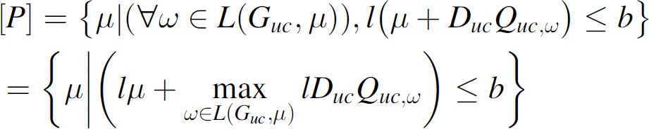
In general, the maximization problem in Eq. (5) is a nonlinear program with an unstructured feasible set L(G _uc , μ). However, a theorem proven in [14] shows that when G is loop free for every state where:

$$\mu \ge 0andQ\ge 0,\mu +DQ\ge 0\iff (\mathrm{\exists }\hspace{0.17em}\omega \in L(G,\mu ))Q=Q_w$$

(6)

The computation of [P] can be reduced to a linear integer program. The set of possible strings ω ∊ L(G, μ) can then be simplified as:

$$\{Q_{uc,\omega }|\omega \in L(G_{uc},\mu )\}=\{Q\in {\mathrm{Z}}^K|\mu +D_{uc}Q\ge 0,Q\ge 0\}$$

(7)

with this simplification of the feasible region, the set [P] of allowed states becomes:

$$[P]=\{\mu |l\mu +l{D}_{uc}{Q}^{\ast }(\mu )\le b\}$$

(8)

where Q∗(μ) is the solution for:

$$\underset{Q}{max}l{D}_{uc}Q\hspace{0.17em}s.t.\{\begin{array}{l}{D}_{uc}Q\ge -\mu \\ Q\ge 0\hspace{0.17em}(\text{int})\end{array}$$

(9)

yielding Q∗ as a function of μ [15].

To confirm the controllability it suffices to test whether or not the initial marking of the system satisfies the equation:

$${\mu }_0\in [P]Or(l{\mu }_0+\underset{\omega \in L(G_{uc},{\mu }_0)}{max}l{D}_{uc}{Q}_{uc,\omega })\le b$$

(10)

If Eq. (10) is not satisfied, no controller exists for this control specification [14].

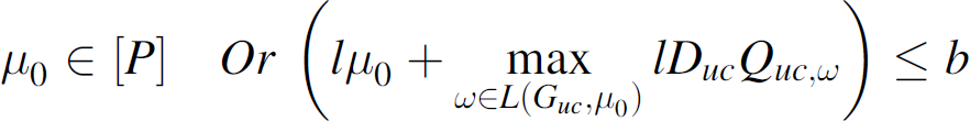
When illegal markings are reachable from the initial marking by passing through a sequence of uncontrollable events, it is an inadmissible specification. Inadmissible control specifications must take an admissible form before synthesizing a controller. Equation (5) is the transformed admissible control specification.

Essentially, a VDES controller is the same as a Petri Net modeled controller. A controller variable c is introduced into the system as a place with the initial value to be b minus the initial value of the transformed admissible control specification [13]. A controllable event will be disabled if and only if its occurrence will make c negative. In our implementation, the controller examines all enabled controllable transitions. If the firing of a transition leads to an illegal state, the system rolls back and continues looking for the next enabled transition.

4.3. Petri Net Based Control

Li and Wonham [13, 14] made significant contributions to the control of plants with uncontrollable events by specifying conditions under which control constraint transformations have a closed form expression. However, the loop free structure of the uncontrollable sub-plant is a sufficient but not necessary condition for control. Moody [10] extended the scope of controller synthesis problems to include unobservable events, in addition to uncontrollable events already discussed in VDES. He also found a method for controller synthesis for plants with loops containing uncontrollable events.

In the Petri Net controller, a plant with n places and m transitions has incidence matrix D _p ∊ Z ^nxm . The controller is a Petri Net with incidence matrix D _c ∊ Z ^{n _c xm} . The controller Petri Net contains all the plant transitions and a set of control places. Control places are used to control the firing of transitions when control specifications will be violated. Control places cannot have arcs incident on unobservable or uncontrollable transitions. Arcs from uncontrollable transitions to control places are permitted. As with VDES, inadmissible control specifications must be converted to admissible control specifications before controller synthesis. An invariant-based control specification: lμ ≤ b is admissible if lD _uc ≤ 0 and lD _uo = 0.

If the original set of control specifications Lμ ≤ b contains inadmissible specifications, it is necessary to define an equivalent set of admissible specifications. Before proceeding with this step, we need to prove that the state space of the new control specifications lies within the state space of the original control specifications. Let R₁ ∊ Z ^n_cxn satisfy R₁μ ≥ 0 ∀μ. Let R₂ ∊ Z ^n_cxn_c be a positive definite diagonal matrix. If

$$L^{\prime }\mu \le b^{\prime }where\begin{array}{l}{L}^{\prime }=R_1+R_{2}L\\ b^{\prime }=R_2(b+1)-1\end{array}$$

(11)

1 is a n _c dimensional vector of 1's, then Lμ ≤ b. The proof is given in [16].

To construct a controller that does not require inhibiting uncontrollable transition or detecting unobservable transitions, it is sufficient to calculate two matrices R₁ and R₂ which satisfy:

$$[R_1\hspace{0.17em}{R}_2]\left[\begin{array}{ll}{D}_{uc}\hspace{0.17em}{D}_{uo}& -D_{uo}\hspace{0.17em}{\mu }_0\\ L{D}_{uc}L{D}_{uo}& -L{D}_{uo}{L}_{{\mu }_0}-b-1\end{array}\right]\le [0\hspace{0.17em}0\hspace{0.17em}0\hspace{0.17em}-1]$$

(12)

The first column in Eq. (12) indicates that LD _uc ≤ 0; the second and the third columns indicate that LD _uo = 0; and the fourth column indicates that the initial marking of the Petri Net satisfies the newly transformed admissible control specification. Using the admissible control specification, a slack variable μ _c is introduced to transform the inequality into an equality:

$$L^{\prime }\mu +{\mu }_c=b^{\prime }$$

(13)

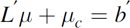
thus,

$$\begin{array}{rl}\hspace{0.5em}& D_c=-(R_1+R_{2}L)D_p=-L^{\prime }{D}_p\\ \hspace{0.5em}& {\mu }_{c0}=R_2(b+1)-1-(R_1+R_{2}L){\mu }_0=b^{\prime }-L^{\prime }{\mu }_0\end{array}$$

(14)

Equation (14) provides the controller incidence matrix and initial marking of the control places.

In contrast with the VDES controller, a Petri Net controller explores the solution by inspecting the incidence matrix. Plant/controller Petri Nets provide a straightforward representation of the relationship between the controller and controlled components. The evolution of the Petri Net plant/controller is inexpensive to compute, which facilitates usage in real time control problems. In our implementation, the plant/controller Petri Net incidence matrix is the output with the plant and control specification as input [16, 17].

4.4. Performance and Comparison of Three Controllers

Figure 3 is an example of a Petri Net consisting of two independent parts with three uncontrollable transitions: T2 a T3 and T5 with an initial marking of [2 0 0 0 1 1 0] ^T . This net is a reduced form of our full-scale DSN design as discussed in sections 2 and 3. The full system and its controller design can be found in the appendix of [11]. The main purpose of this reduced example is to simply illustrate how the control issues are handled in our DSN. The results of the three approaches and comparison are given.

Figure 3.

A reduced DSN Petri Net model.

The behavior of the two independent Petri Nets should obey the control specifications. The first constraint requires that place P5 cannot contain more than two tokens. There cannot be more than two processes active at one time. The second constraint states that the sum of tokens in P2 and P6 must be less or equal 1. This constraint implies that when a node is in sensing status in the collaborative sensing hierarchy, it is not allowed to move in the operational command hierarchy or vice versa. This mutual exclusion constraint represents the major control task of enforcing consistency across independently evolving hierarchies in our DSN. Three uncontrollable transitions are sensing complete, interpreting complete, and moving complete.

Two control specifications in inequality forms:

μ₅ ≤ 2

μ₂ + μ₆ ≤ 1

4.5. Finite State Machine Controller

A reachability tree has thus been constructed from Petri Net. Table 1 shows all states generated from the Plant without constraints. We intentionally omit portions of the Karp-Miller tree in order to save space. After converting all inadmissible control specifications to admissible ones, we search the entire state space. Removing illegal states yields a new state space with 13 legal states as shown in Table 2. Four bits are needed to encode 13 states as encoded by A, B, C, and D. A Moore machine is constructed to output the binary control pattern based on the current encoded state in Table 3.

TABLE 1

All States Generated from the plant

States {
s2_0_0_0_1_1_0,	s0_0_0_2_3_0_1,	s1_1_2_0_0_1_0,
s1_1_1_0_1_1_0,	s1_0_0_1_2_0_1,	s0_2_3_0_0_1_0,
s0_2_2_0_1_1_0,	s0_1_1_1_2_0_1,	s0_2_3_0_0_0_1,
s0_1_2_1_1_1_0,	s0_0_1_2_2_0_1,	s0_2_2_0_1_0_1,
s0_0_2_2_1_1_0,	s1_0_1_1_1_0_1,	s0_2_1_0_2_0_1,
s0_0_1_2_2_1_0,	s0_1_2_1_1_0_1,	s1_1_2_0_0_0_1,
s0_0_0_2_3_1_0,	s0_0_2_2_1_0_1,	s1_1_1_0_1_0_1,
s1_0_0_1_2_1_0,	s1_0_2_1_0_0_1,	s1_1_0_0_2_0_1,
s0_1_1_1_2_1_0,	s0_1_3_1_0_0_1,	s2_0_1_0_0_0_1,
s0_1_0_1_3_1_0,	s0_0_3_2_0_0_1,	s2_0_0_0_1_0_1
s1_1_0_0_2_1_0,	s0_0_3_2_0_1_0,	}
s0_2_1_0_2_1_0,	s0_1_3_1_0_1_0,
s0_2_0_0_3_1_0,	s1_0_2_1_0_1_0,
s0_2_0_0_3_0_1,	s1_0_1_1_1_1_0,
s0_1_0_1_3_0_1,	s2_0_1_0_0_1_0,

TABLE 2

All Legal States and Encoded States

States: Marking	Encode States
State S0: 2000110	0000
State S1: 2000101	0001
State S2: 1110101	0010
State S3: 1011101	0011
State S4: 1001201	0100
State S5: 1001210	0101
State S6: 2010001	0110
State S7: 1120001	0111
State S8: 1021001	1000
State S9: 1021010	1001
State S10: 1011110	1010
State S11: 2010010	1011
State S12: 1100201	1100

TABLE 3

Transition Table with Encoded States for Moore Machine

Present state	Next State						Output	Output
ABCD (Encoded Bits)	T1	T2	T3	T4	T5	T6	T1	T6
S0					S1		0	1
S1	S2					S0	1	1
S2		S3	S12				0	0
S3			S4	S6	S10	0	1
S4				S1		S5	0	1
S5				S0	S4		0	1
S6	S7		S1			S11	1	1
S7		S8	S2				0	0
S8			S3			S9	0	1
S9			S10		S8		0	1
S10			S5	S11	S3	0	1
S11			S0		S6		0	1
S12		S4					0	0

Among six transitions, we cannot control T2, T3, or T5. Those controllable transitions whose firings would lead to an illegal state directly or indirectly will be controlled. Based on the knowledge of offline screening, T1 and T6 should be controlled. Thus, the binary control pattern has two bits. Table 2 shows the transition table with encoded states for Moore machine:

From the transition table, we can construct a Moore machine state diagram with 13 states, 6 inputs, and two output variables in Table 3. The state feedback function, which outputs the binary control patterns based on the current state, is used to regulate plant behavior by switching between control patterns.

The logical expression of the binary control pattern can be expressed as: $\{\begin{array}{l}{T}_1=\bar{A}\bar{B}\bar{C}D+\bar{A}BC\bar{D}\\ \overline{T_6}=\bar{A}C(\overline{BD}+BD)+AB\bar{C}\bar{D}\end{array}$ Logical implementation can be realized by hardware. The controller can immediately access the control pattern for each controllable transition based on the current encoded state without going through legal firing checking as in VDES or doing extra calculation involving added controller places and arcs as in the Petri Net Modeled controller. The trade-off is offline legal state space searching. Following our search method used in the DSN, we simply check whether or not the current state vector satisfies the conjunction of: μ₃ + μ₅ ≤ 1 and μ₂ + μ₆ = 0. If yes, the control pattern bit of T1 is 1. If μ₂ + μ₆ = 0, the control pattern bit of T6 is 1. It turns out to be computation and expression efficient for a complex system.

4.6. Vector Discrete Event System Modeled Controller

$$D=\left[\begin{array}{rrrrrr}-1& 0& 0& 1& 0& 0\\ 1& -1& 0& 0& 0& 0\\ 1& 0& -1& 0& 0& 0\\ 0& 1& 0& -1& 0& 0\\ 0& 0& 1& -1& 0& 0\\ 0& 0& 0& 0& -1& 1\\ 0& 0& 0& 0& 1& -1\end{array}\right]D_{uc}=\left[\begin{array}{rrr}0& 0& 0\\ -1& 0& 0\\ 0& -1& 0\\ 1& 0& 0\\ 0& 1& 0\\ 0& 0& -1\\ 0& 0& 1\end{array}\right]$$

The controller goal is to enforce linear inequality on the state vector of G, usually in the form of lμ ≤ b. Our control specifications are μ₅ ≤ 2 and μ₂ + μ₆ ≤ 1 let us consider the first control specification,

$$l_1=[0\hspace{0.17em}0\hspace{0.17em}0\hspace{0.17em}0\hspace{0.17em}1\hspace{0.17em}0\hspace{0.17em}0]b_1=2.$$

The initial marking satisfies the control specification, but the control specification is inadmissible because the uncontrollable firing of T₃would lead to a violation. Since the uncontrollable part of the system is loop free the inadmissible control specification can be transformed to an admissible control specification. Solve the $\underset{Q}{\max }l{D}_{uc}Q$

$$s.t.\{\begin{array}{l}{D}_{uc}Q\ge -\mu \\ Q\ge 0\hspace{0.17em}(\text{int})\end{array}$$

$$\underset{Q}{max}{l}_1{D}_{uc}Q=[0\hspace{0.17em}0\hspace{0.17em}0\hspace{0.17em}0\hspace{0.17em}1\hspace{0.17em}0\hspace{0.17em}0]\left[\begin{array}{rrr}0& 0& 0\\ -1& 0& 0\\ 0& -1& 0\\ 1& 0& 0\\ 0& 1& 0\\ 0& 0& -1\\ 0& 0& 1\end{array}\right]\left[\begin{array}{c}{q}_2\\ q_3\\ q_5\end{array}\right]=max(q_3)$$

$$s.t\{\begin{array}{l}\left[\begin{array}{rrr}0& 0& 0\\ -1& 0& 0\\ 0& -1& 0\\ 1& 0& 0\\ 0& 1& 0\\ 0& 0& -1\\ 0& 0& 1\end{array}\right]\left[\begin{array}{c}{q}_2\\ q_3\\ q_5\end{array}\right]\ge \left[\begin{array}{c}-{\mu }_1\\ -{\mu }_2\\ -{\mu }_3\\ -{\mu }_4\\ -{\mu }_5\\ -{\mu }_6\\ -{\mu }_7\end{array}\right]\Rightarrow \\ q_i\ge 0\end{array}\{\begin{array}{l}-{\mu }_1\le 0\\ {\mu }_2\ge q_2\\ {\mu }_3\ge q_3\\ -{\mu }_4\le q_2\\ -{\mu }_5\le q_3\\ {\mu }_6\ge q_5\\ -{\mu }_7\le q_5\end{array}$$

From above, it can be inferred that max (q₃) equals μ₃, as μ₃ ≥ q₃. The transformed admissible control specification is lμ + max lD _uc .∗(μ) ≤ b, which is μ₅ + μ₃ ≤ 2. The initial marking [2 0 0 0 1 1 0] ^T holds for μ₅ + μ₃ ≤ 2, thus the controller exists for this control constraint [15]. The second control specification is an admissible one, because no uncontrollable transition firing would lead to an illegal state.

In our controller implementation, the plant together with two admissible control specifications, are treated as input. The state space of the controlled system is the following:

$$\begin{array}{l}2\mathrm{\_}0\mathrm{\_}0\mathrm{\_}0\mathrm{\_}1\mathrm{\_}1\mathrm{\_}0,1\mathrm{\_}1\mathrm{\_}2\mathrm{\_}0\mathrm{\_}0\mathrm{\_}0\mathrm{\_}1,\\ 2\mathrm{\_}0\mathrm{\_}0\mathrm{\_}0\mathrm{\_}1\mathrm{\_}0\mathrm{\_}1,1\mathrm{\_}0\mathrm{\_}2\mathrm{\_}1\mathrm{\_}0\mathrm{\_}0\mathrm{\_}1,\\ 1\mathrm{\_}1\mathrm{\_}1\mathrm{\_}0\mathrm{\_}1\mathrm{\_}0\mathrm{\_}1,1\mathrm{\_}0\mathrm{\_}2\mathrm{\_}1\mathrm{\_}0\mathrm{\_}1\mathrm{\_}0,\\ 1\mathrm{\_}0\mathrm{\_}1\mathrm{\_}1\mathrm{\_}1\mathrm{\_}0\mathrm{\_}1,1\mathrm{\_}0\mathrm{\_}1\mathrm{\_}1\mathrm{\_}1\mathrm{\_}1\mathrm{\_}0,\\ 1\mathrm{\_}0\mathrm{\_}0\mathrm{\_}1\mathrm{\_}2\mathrm{\_}0\mathrm{\_}1,2\mathrm{\_}0\mathrm{\_}1\mathrm{\_}0\mathrm{\_}0\mathrm{\_}1\mathrm{\_}0,\\ 1\mathrm{\_}0\mathrm{\_}0\mathrm{\_}1\mathrm{\_}2\mathrm{\_}1\mathrm{\_}0,1\mathrm{\_}1\mathrm{\_}0\mathrm{\_}0\mathrm{\_}2\mathrm{\_}0\mathrm{\_}1\\ 2\mathrm{\_}0\mathrm{\_}1\mathrm{\_}0\mathrm{\_}0\mathrm{\_}0\mathrm{\_}1,\end{array}$$

∗

All these states satisfy two control specifications.

4.7. Petri Net Modeled Controller

We have the same first control specification as μ₅ ≤ 2. As the plant has no unobservable transitions, we only need to study uncontrollable transitions. The first step is to determine if the control specification is admissible.

$$[0\hspace{0.17em}0\hspace{0.17em}0\hspace{0.17em}0\hspace{0.17em}1\hspace{0.17em}0\hspace{0.17em}0]D_{uc}=[0\hspace{0.17em}1\hspace{0.17em}0]\ge [0\hspace{0.17em}0\hspace{0.17em}0]$$

Indicating an inadmissible control specification as discussed before.

It was observed that the third row of D _uc as [0 − 1 0] could be used to eliminate the positive element 1 in the above equation. So,

$$\begin{array}{c}{R}_1=[0\hspace{0.17em}0\hspace{0.17em}1\hspace{0.17em}0\hspace{0.17em}0\hspace{0.17em}0\hspace{0.17em}0]R_2=1\\ L^{\prime }=R_1+R_{2}L=[0\hspace{0.17em}0\hspace{0.17em}1\hspace{0.17em}0\hspace{0.17em}0\hspace{0.17em}0\hspace{0.17em}0]+1[0\hspace{0.17em}0\hspace{0.17em}0\hspace{0.17em}0\hspace{0.17em}1\hspace{0.17em}0\hspace{0.17em}0]=[0\hspace{0.17em}0\hspace{0.17em}1\hspace{0.17em}0\hspace{0.17em}1\hspace{0.17em}0\hspace{0.17em}0]\end{array}$$

The initial marking satisfies the admissible control specification. The transformed admissible control specification is: μ₅ + μ₃ ≤ 2, which is the same as the admissible control specification from the above section. By introducing a new slack variable μ _c , the control specification becomes equality.

$${\mu }_5+{\mu }_3+{\mu }_c=2$$

∗

For the second admissible control specification: μ₂ + μ₆ ≤ 1, we introduce another slack variable μ^′ _c , and the second control specification becomes another equality.

$$\begin{array}{rl}\hspace{0.5em}& {\mu }_2+{\mu }_6+{\mu }_c^{\prime }=1\\ \hspace{0.5em}& D=\left[\begin{array}{rrrrrr}-1& 0& 0& 1& 0& 0\\ 1& -1& 0& 0& 0& 0\\ 1& 0& -1& 0& 0& 0\\ 0& 1& 0& -1& 0& 0\\ 0& 0& 1& -1& 0& 0\\ 0& 0& 0& 0& -1& 1\\ 0& 0& 0& 0& 1& -1\end{array}\right]{\mu }_0=[2000110{]}^T\\ \hspace{0.5em}& L=\left[\begin{array}{c}0\hspace{0.17em}0\hspace{0.17em}1\hspace{0.17em}0\hspace{0.17em}1\hspace{0.17em}0\hspace{0.17em}0\\ 0\hspace{0.17em}1\hspace{0.17em}0\hspace{0.17em}0\hspace{0.17em}0\hspace{0.17em}1\hspace{0.17em}0\end{array}\right]b=\left[\begin{array}{c}2\\ 1\end{array}\right]\\ \hspace{0.5em}& D_c=-LD=\left[\begin{array}{rrrrrr}-1& 0& 0& 1& 0& 0\\ -1& 1& 0& 0& 1& -1\end{array}\right]and\\ \hspace{0.5em}& {\mu }_{c0}=b-L{\mu }_0=\left[\begin{array}{c}2\\ 1\end{array}\right]-\left[\begin{array}{c}1\\ 1\end{array}\right]=\left[\begin{array}{c}1\\ 0\end{array}\right]\end{array}$$

The resulting overall plant/controller incidence matrix is

$$D_{all}=\left[\begin{array}{rrrrrr}-1& 0& 0& 1& 0& 0\\ 1& -1& 0& 0& 0& 0\\ 1& 0& -1& 0& 0& 0\\ 0& 1& 0& -1& 0& 0\\ 0& 0& 1& -1& 0& 0\\ 0& 0& 0& 0& -1& 1\\ 0& 0& 0& 0& 1& -1\\ -1& 0& 0& 1& 0& 0\\ -1& 1& 0& 0& 1& -1\end{array}\right]$$

Two controller places can be added to the plant as P8 and P9 with initial marking of 1 and 0, respectively, as shown in Fig. 4. In our implementation, the Petri Net modeled controller implementation computes a closed loop Petri Net incidence matrix based on the plant and the control constraints to be enforced without going through the above manual computation.

Figure 4.

Plant/Controller Petri Net model.

Running our implementation program, we get a FSM as shown below:

All these states are legal.

5. Simulation Results

Software was developed to simulate the actions of a Distributing Sensing Network represented by a Petri Net plant model. The constraints listed were those to be monitored and enforced by each of the controllers. The full-scale Petri Net plant model of the DSN consisted of 133 places, 234 transitions, and roughly 1000 arcs. In order to enforce the plain language constraints, 44 inequalities of the form lμ ≤ b were generated. FSM controller is not simulated due to high manual representation and offline computation costs for a large system.

The Petri Net controller was implemented automatically by creating 44 control places that would act as the slack variables in a closed loop Petri Net. Arcs from these controller places influence controllable transitions in the plant net in an effort to enforce the constraints. Thus the controlled plant Petri net is simply a new Petri Net with additional places and arcs. Unlike the Petri Net controller, the VDES controller required no additional places or arcs to control the plant net. The VDES controller was implemented by examining every possible enabled firing given a plant state. The controller then examined the state of the system should each of these enabled firings take place, and disabled those transitions whose firings led to a forbidden state. This characteristic of VDES control illustrates a similarity with Moore machines. In Moore machines, the entire state space is explored offline and all forbidden strings are known a priori. In the case of VDES, exploration of reachable states is undertaken at each state dynamically and is limited to those states directly reachable from the current state.

The plant model was activated and the set of forbidden states were monitored at each transition firing. Without a controller of any kind in place, the plant model reached a forbidden state in less than 10,000 transition firings in each test. When the Petri Net or the VDES controllers were implemented, the plant model ran through 100,000 transition firings without violation. Thus, each controller was found to be effective in preventing the violation of system constraints, and the choice of which to use can be based upon issues such as execution speed. It was found that the relationship between the initial state and the controller specification was crucial. In complex systems such as the DSN, it is not difficult to specify an initial marking that will make the plant uncontrollable. Care must be taken to ensure that the system design and marking do not render the controller useless.

The simulation results show that the system behavior is similarly and effectively constrained by any of the three approaches. Secondary concerns such as execution time and ease of representation can therefore guide decision on which approach to use.

6. Conclusion

Faced with the problem of synthesizing a controller for our large-scale surveillance network, we selected three methods as candidates and applied them to our system. Through comparison, we concluded that the approaches are roughly equivalent, each with pros and cons. Comparison is conducted mainly from the aspects of computation cost, real time response time, and representation space.

The traditional RW control model is based on a classic finite automaton. Unfortunately, FSM based controllers involve exhaustive searches or simulation of system behavior and are especially impractical for large and complex systems. We eliminate illegal state spaces before synthesizing our finite automata, but the process is still a computationally expensive one for a system with a large number of states and events. Offline searching of the entire set of reachable states and the hardware logical expression implementation assures prompt controller response, which is crucial for those systems with strict real-time requirements. For a complex system such as a surveillance system, we use a modified version of an FSM modeled controller to avoid expensive computation and high representation cost. The controller is directly derived from the control specifications.

On the contrary, Petri Net based controllers take full advantage of the properties of the Petri Net. Their efficient mathematical computation employing linear matrix algebra makes real-time controlling and analysis possible, but they are still inferior to FSM in the performance of response time. Petri Nets offer a much more compact state space than finite automata and are better suited to model systems with repeated structure. Automatic handling of concurrent events is maintained as shown in [15,16].

Vector discrete event system controllers explore the maximally permissive control constraint on the Petri Net with uncontrollable transitions by application of integer linear programming problem, assuming that the uncontrollable portion of the Petri Net has no loops and the actual controller exists [16]. However, VDES does not consider unobservable events. The loop-free condition proves to be a sufficient, but not a necessary condition. Petri Net modeled controllers investigate the structural properties of a controlled Petri Net with unobservable events in addition to uncontrollable events. The integrated graphical structure of the Petri Net plant/controller makes system computation and representation straightforward.