Suppressing Temporal Data in Sensor Networks Using a Scheme Robust to Aberrant Readings

Abstract

The main goal of a data collection protocol for sensor networks is to keep the network's database updated while saving the nodes' energy as much as possible. To achieve this goal without continuous reporting, data suppression is a key strategy. The basic idea behind data suppression schemes is to send data to the base station only when the nodes' readings are different from what both the nodes and the base station expect. Data suppression schemes can be sensitive to aberrant readings, since these outlying observations mean a change in the expected behavior for the data. Transmitting these erroneous readings is a waste of energy. In this article, we present a temporal suppression scheme that is robust to aberrant readings. We use a technique to detect outliers from a time series. Our proposal classifies the detected outliers as aberrant readings or change-points using a post-monitoring window. This idea is the basis for TS-SOUND (Temporal Suppression by Statistical OUtlier Notice and Detection). TS-SOUND detects outliers in the sequence of sensor readings and sends data to the base station only when a change-point is detected. Therefore, TS-SOUND filters aberrant readings and, even when this filter fails, TS-SOUND does not send the deviated reading to the base station. Experiments with real and simulated data have shown that the TS-SOUND scheme is more robust to aberrant readings than other temporal suppression schemes (value-based, PAQ and exponential regression). Furthermore, TS-SOUND has got suppression rates comparable or greater than the rates of the cited schemes, in addition to keeping the prediction errors at acceptable levels.

1. Introduction

Sensor networks are a powerful instrument for data collection, especially for applications like habitat and environmental monitoring. These applications often require continuous updates of the database at the network's root. However, sending continuous reports would quickly run out the limited energy of the nodes. A solution for continuous updating without continuous reporting is to use data suppression [1].

The first author was partially supported by CAPES under PICDT program. The authors thank to the anonymous reviewers for their excellent suggestions, which have contributed to improve this article.

To define a data suppression scheme, the nodes and the base station have to agree on an expected behavior for the nodes' readings. Thus, if the nodes' readings fit the expected behavior, the nodes suppress these data. Otherwise, when their sensed values do not fit the expected behavior, nodes send reports to the base station. These reports are used to predict the suppressed data.

Suppression schemes are an alternative to improve the reactivity of a sensor network, which is defined as the ability of a network to react to its environment providing only relevant data [2]. Instead of changing the sampling rates according to the sampled values and sending all collected data to the base station as in [2], a suppression scheme collects data using a constant rate. However, it only sends data if they represent a deviation from the behavior agreed by the nodes and the base station.

Model-driven data suppression [3] defines the mean of a node's observations as their expected behavior and models this mean using temporal or spatio-temporal correlations.

A temporal data suppression scheme uses the correlation among the readings of a same node to build the expected behavior for the nodes' readings [4]. A spatio-temporal suppression scheme also considers the correlation among the observations of neighboring nodes [1].

Usually, suppression schemes define an absolute error measure to evaluate the deviation between sensed data and their expected behavior. This produces data collection schemes that are sensitive to aberrant readings. These outlying values can be the result of a temporary malfunctioning of a particular sensor or due to some intervention in the environment on which the network is operating and it does not have any relation with the monitored variables. Sometimes, aberrant readings can be the result of an expected change in the sensed values. For instance, solar radiation measurements often suffer the effect of temporary clouds. In this case, a reduction in the radiation values is expected and, perhaps, non-interesting to the network user.

Sensors measuring environmental variables can produce such erroneous or nonsense readings [5–10], particularly in outdoor applications [11, 12]. In monitoring networks with low energy constraints, such as the regular weather stations, the nodes transmit or record the aberrant readings, which are identified and deleted in the base station. However, for a sensor network, transmitting nonsense values means to waste valuable resources.

In this article, we propose a temporal suppression scheme that is robust to aberrant readings. Our proposal is based on the detection of outliers and their posterior classification into change-points or aberrant readings. We consider the sequence of data collected by a node as observations of a temporal process. The probabilistic distribution of this process at each time period is used to infer about the expected behavior of the observations. An outlier is an observation that presents a small probability to belong to the distribution at the current time period. An outlier reading may suggest a change in the expected value for the time series or it may be an aberrant reading.

To detect outliers from a time series, we have adapted the proposal in [13]. We have inserted our version as part of a suppression scheme for data collection in sensor networks, the TS-SOUND scheme (Temporal Suppression by Statistical OUtlier Notice and Detection). After detecting an outlier, the TS-SOUND classifies it into a change-point or an aberrant reading. In the former case, the node sends data to the base station. Otherwise, the node suppresses its data.

We have designed TS-SOUND for applications that are not interested in aberrant readings, since they represent a failure in data sensing or processing. Usually, these erroneous measurements occur at random, isolated or clustered. If they remain, this means malfunctioning and suggests a nonreliable node.

The TS-SOUND scheme adopts a procedure to avoid detecting an aberrant reading as a change-point. Furthermore, even if this misdetection occurs, the TS-SOUND does not send the aberrant reading to the base station.

In this article, we claim and demonstrate that our proposed scheme for temporal suppression data is robust to aberrant readings. Furthermore, considering the trade-off between energy consumption and data quality, TS-SOUND has outperformed the model-based suppression schemes we have considered in this article (PAQ [4] and exponential regression [1]) and also the simplest data suppression scheme, VB scheme [1]. The prediction error measures the quality of the data sent to the base station. Since the data transmission is the most important energy consumer, we use the suppression rates as a proxy for the energy consumption. To evaluate the TS-SOUND scheme, we have run evaluation experiments with real and simulated data.

The remainder of this article is organized as follows. Section 2 presents a TS-SOUND overview. In Section 3, we describe the related work and the framework for suppression schemes proposed in [1]. Section 4 describes SDAR algorithm [13], which allows for the on-line estimation of time series parameters. In addition, it describes the procedure in [13] to detect outliers, how we have adapted it to be part of our proposed suppression scheme, and how the TS-SOUND deals with classifying the outliers into change-points or aberrant readings. In Section 5, we present the TS-SOUND protocol and frame it as a suppression scheme according to the proposal in [1]. Section 6 describes the evaluation experiments and Section 7 presents their results using real and simulated data. Finally, Section 8 discusses the experiments results and Section 9 presents some future directions.

2. TS-SOUND Overview

Techniques for outlier detection have been proposed in communities as Statistical Process Control (for example [14, 15]), Data Mining, and Database and Machine Learning (for example [13, 16–18]).

In Statistical Process Control (SPC), for instance, the goal is to monitor a process initially “in-control” and raise an alarm when this process is considered to be “out-of-control” as soon as possible. Often, the “in-control” state of the process is a predefined condition: nominal values for the monitored parameters and their tolerance bounds. To raise the alarm, SPC uses procedures to detect outliers.

For TS-SOUND, the “in-control” state is the probabilistic distribution of the monitored variable at the last time period. If the process is “in-control” during a time interval, the sensor readings follow the same probabilistic distribution along this interval and different values are caused by random fluctuation around an expected value. Then, we can suppress these readings. We consider the process is “out-of-control” if the expected value of this distribution changes. After the change, a new “in-control” state is defined. The change's relevancy is a user-defined parameter.

As in the SPC techniques, the TS-SOUND uses the outlier occurrence to infer if the process is “out-of-control.” To detect outliers, the TS-SOUND adapts the technique in [13], which has been proposed to detect outliers from a time series. TS-SOUND employs an algorithm that considers the temporal dependence of the time series to update the parameters of the probability distribution at each new sensor reading (on-line estimation). This algorithm is called SDAR (Sequentially Discounting Auto-Regressive) [13]. SDAR combines the last parameters' updates with the new sensor reading to produce the new parameters' updates. SDAR uses a discounting factor to control the weight of the new sensor data in the updates' values. The outliers are detected as deviations from the data distribution.

In a time series, an outlier can suggest a distribution change-point or an aberrant reading. We can distinguish a change-point from an aberrant reading if we compare the time series values before and after the outlier, examining, for instance, the time series plot (Fig. 1). The aberrant points appear as the “peaks” or “spikes” of the time series plot. The time series has similar behaviors before and after the occurrence of aberrant readings. On the other hand, after a change-point, the time series changes its behavior. Then, a data suppression scheme must update the database at the base station only when change-points occur.

Figure 1.

Outliers in a wind speed time series (black dots)

To distinguish change-points from aberrant readings, the TS-SOUND opens a post-monitoring window whenever it detects an outlier. During this time interval, the node keeps collecting data and updating the estimated distribution parameters. At the end of this time window, the TS-SOUND compares the collected values with the distribution before and after the detected outlier. This outlier is classified as a change-point if the post-monitoring data are considered to be:

discrepant readings in relation to the distribution before the outlier;

nondiscrepant readings in relation to distribution after the outlier.

If the TS-SOUND classifies the detected outlier as a change-point, it summarizes the data collected during the post-monitoring and sends the result to the base station. We have adopted a post-monitoring window for two reasons:

to be able to distinguish change-points from aberrant readings. It avoids sending the latter ones to the base station;

to allow for capturing the value of the new expected behavior through the summary of the collected values.

The base station uses the last sent data as an estimate for the node's readings until it receives a message with new data. Thus, for each node in the network, the base station stores a sequence of summaries and uses this time series as an estimate for the real node's time series. Section 5 describes the TS-SOUND suppression scheme in detail.

3. Related Work

In this section, we describe the work related to our proposal considering two distinct topics: data suppression schemes for sensor networks and outliers detection in sensor networks.

Section 3.1 describes some proposals for temporal data suppression schemes and relates them to our proposal. In Section 3.2, we describe a proposal for a general framework for data suppression schemes [1]. This framework makes the comparisons among data suppression schemes easier. We use the proposal in [1] to frame TS-SOUND as a data suppression scheme in Section 5.4.

Since TS-SOUND uses outliers detection as the basis for its suppression scheme, Section 3.3 provides a brief review of previous works on detecting outliers in a sensor network.

3.1. Temporal Data Suppression Schemes

Recently, some protocols for data suppression in sensor networks have proposed to use statistical models to predict the nodes' data at the base station reducing the amount of communication inside the network. This approach to data suppression is called model-driven [3].

The main idea in [3] is to keep synchronized two probabilistic models: one at base station and the other at the nodes. The model parameters are estimated in a learning phase. Based on these identical models, the nodes and the base station make the same predictions on the data to be collected. Then, the node collects the actual data and compares them to its prediction. If the difference between the real and predicted values is greater than a user-defined error bound, the node sends its data to the base station. Otherwise, the node suppresses the collected data.

A similar idea appears in [4]. The PAQ protocol makes predictions based on a time series model, the third-order autoregressive model, AR(3). Given a time period t, the predicted value in t is written as a linear combination of the last three observations before t. PAQ uses two predefined error bounds to monitor the prediction error, defined as the absolute difference between the real and the predicted value. When the prediction error is greater than ε_υ, PAQ considers the observation as an outlier and sends it to the base station. If the prediction error is smaller than ε_υ but it is greater than ε_δ (ε_δ < ε_υ), PAQ opens a monitoring window. During the next A_PAQ time periods, the node goes on collecting data, predicting their values and monitoring outliers, sending these last ones to the base station. At the end of the monitoring window, PAQ counts how many observations have had prediction errors greater than ε_υ or greater than ε_δ but smaller than ε_υ. If this sum is greater than a threshold a (a ≤ A_PAQ), PAQ decides to relearn the four model parameters. Then, PAQ calculates their new values and sends them to the base station. A variation of PAQ, called in [1] as exponential regression (EXP), uses the observation in the time period (t − 1) in a simple linear regression to predict the observation in t. Thus, EXP has to estimate two model parameters.

It is worth mentioning that, differently from TS-SOUND, neither PAQ nor EXP distinguishes a change-point from an aberrant reading. Once they detect an outlier reading, the node sends the observation to the base station, even if it is an aberration.

3.2. A Framework for Data Suppression Schemes

According to Silberstein et al. [1], the nodes in the network are classified into updaters and observers. A suppression link describes the suppression/reporting relationship between an updater and its observer. The set of suppression links within the sensor network defines a suppression scheme.

In a simple suppression scheme, all the network nodes are updaters. These updaters collect data and decide to send them (or not) to the observer node, which is the base station. To produce a report r_t to its observer, the updater uses an encoding function f_enc. To decode the updater report, the observer uses a decoding function.

The vector X_t represents the data of the updater node at time period t and the vector ${\hat{\mathrm{X}}}_{\mathrm{t}}$ represents the data as calculated by the observer node at the same time period. The suppression link maintains X_t and ${\hat{\mathrm{X}}}_{\mathrm{t}}$ synchronized by evaluating a function $g({\mathrm{X}}_{\mathrm{t}},{\hat{\mathrm{X}}}_{\mathrm{t}})$ . The function g returns the logical TRUE value if ${\hat{\mathrm{X}}}_{\mathrm{t}}$ is within a user-defined error tolerance (ε) of X_t.

In a Value-Based (VB) suppression scheme, for instance, the encoding and decoding functions are defined by (1) and (2), respectively,

$$f_{\text{enc}}=\{\begin{array}{ll}{x}_t-x_t,& \text{if}\hspace{0.17em}|x_t-x_t|>{\epsilon }_{VB}\\ \perp ,& \text{otherwise}\end{array}$$

(1)

$${\hat{x}}_t=\{\begin{array}{ll}{\hat{x}}_{(t-1)}+r_t& \text{if}\hspace{0.17em}{r}_t=x_t-x_t\\ {\hat{x}}_{(t-1)},& \text{if}\hspace{0.17em}{r}_t=\perp \end{array}$$

(2)

where x_t is a component of the vector X_t, t' is the last time the updater sends a message to its observer, and the symbol ⊥ represents data suppression. The value x_t′ is what the observer knows about its updater at time period t. If the relative difference between the current updater value x_t and x_t′, the g function is greater than error bound ε_VB, the updater produces a report r_t = x_t-x_t, and sends it to the observer node. Otherwise, no message is sent (r_t = ⊥). The observer computes its value ${\hat{x}}_t$ by adding the received report r_t to its old value ${\hat{x}}_{t-1}$ . If the updater does not send a message, the observer updates ${\hat{x}}_t$ by repeating the old value.

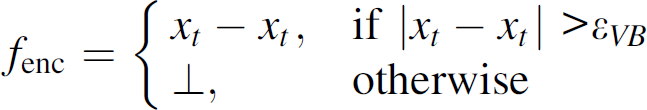
PAQ and exponential regression have also been framed as temporal suppression schemes. Although PAQ also has a proposal for spatio-temporal suppression [4], we just consider its temporal version in this article. The expressions in (3) and (4) reproduce the encoding functions of PAQ and EXP, respectively,

$$f_{\text{enc}}=\{\begin{array}{ll}{\alpha }_t,{\beta }_t,{\gamma }_t,{\eta }_t& \text{if}\hspace{0.17em}(model\hspace{0.17em}RElearn)\\ x_t& \text{if}\hspace{0.17em}(outlier)\\ \perp & \text{otherwise}\end{array},$$

(3)

$$f_{\text{enc}}=\{\begin{array}{ll}{\alpha }_t,{\beta }_t& \text{if}\hspace{0.17em}(model\hspace{0.17em}RElearn)\\ x_t& \text{if}\hspace{0.17em}(outlier)\\ \perp & \text{otherwise}\end{array}.$$

(4)

In (3), α_t, β_t, γ_t, and η_t are the coefficients of the AR(3) model adopted by PAQ scheme and, in (4), α_t and β_t are the coefficients of the simple linear regression model adopted by EXP scheme. The functions modelRelearn and outlier enclose the g function of PAQ and EXP schemes. As in the VB scheme, it also evaluates the error between the real and the predicted values.

We classify our TS-SOUND proposal as a model-driven approach for temporal suppression [1]. TS-SOUND models the mean of the monitored variable and uses it to decide if an observation is an outlier of the current data distribution. However, the model runs only at the nodes, not at the base station, being not necessary to keep synchronized models as in the other model-driven proposals. We frame the TS-SOUND approach as a temporal suppression scheme in Section 5.4.

3.3. Outliers Detection in a Sensor Network

Recently, the problem of detecting outliers in a sensor network has gained importance [5] and generated works such as [6–10]. The proposal in [6] removes outlier readings from the data aggregation. Differently from the TS-SOUND, the proposal in [6] makes the outliers available to the monitoring application. In [7], the authors detect outliers within a sliding window that holds the last W values of the sensor data. To estimate the data distribution, they use nonparametric models. As in [6], they report the outlier readings to the base station. However, this is done through a hierarchical structure, using the union of the outliers coming from multiple sensors. The authors in [8] propose a generic distributed algorithm that accommodates many nonparametric methods to detect outliers such as the “distance to the k^th nearest neighbor” and the “average distance to the k nearest neighbors.” Nodes use one of these techniques to find out their local outliers and exchange information about them with their neighboring nodes to find out global outliers. In [9], the authors propose to use kernel density estimators to approximate the data distribution at each sensor node. As the SDAR algorithm in [13], the kernel density estimation allows for adjusting itself to the input data distribution, as this distribution changes overtime. The proposal in [9] assumes a heterogeneous sensor network, in which few sensor nodes are more powerful than the other sensors in the network. The detection of outliers is performed by these empowered nodes, which combine the models of two or more sensor nodes in this task. The authors discuss the trade-off among data accuracy, the number of updates, and the size of the estimation models in some application scenarios. However, they do not provide evaluation experiments to show how this would work on real data. In [10], the authors propose to identify local outliers using temporal and spatial autocorrelations among nodes' values. Using the “distance” between its current value and its past values, a node is able to identify a potential (temporal) outlier comparing the “distance” with a learned distance threshold. If a potential outlier is detected, the node uses the distance threshold of its neighbors to finally classify its current value as an outlier (or not). The “distance” measurement can be done using several types of functions. The authors in [10] also propose to classify the detected outliers into error or events, which could be equivalent to what we call aberrant readings and change-points, respectively. If a node observes an outlier due to an event, the authors argue that most of the node's neighborhood should also detect outliers, since the value of the neighboring nodes are spatially correlated. Then, summarizing the idea in [10], if a node classifies its current value as an outlier and most of its neighboring nodes also classify their current values as outliers, the node's value is considered to be an event.

Differently from the proposals described above, our proposal to detect outliers does not require communication among sensor nodes, since we have treated only the temporal aspect of the data suppression in this article. Moreover, except by the proposal in [10], the described proposal is not concerned about classifying the detected outlier into aberrant readings or change-points. However, some described proposals can be an interesting basis for a future spatio-temporal version of TS-SOUND scheme.

An extensive survey of outliers detection techniques for sensor networks is not our aim. For a comprehensive overview on this subject, we refer to the work in [5].

4. Detecting Outliers from a Time Series

In this section, we present the procedure in [13] to detect outliers from a time series and our proposal for adapting it to the constrained environment of a sensor network.

We consider the sequence of the data sensed by a sensor node, {X_t, t = 1,2,3 …}, as a time series.

The autoregressive (AR) model is the simplest model to represent the statistical behavior of a time series. In AR(k), the autoregressive model of order k, the observation at time t, X _t , is written as a combination of the last k past observations as the following

$$\begin{array}{rl}{X}_t=\mu & \hspace{0.5em}+{\rho }_1(X_{t-1}-\mu )+{\rho }_2(X_{t-2}-\mu )+\dots \\ \hspace{0.5em}& \hspace{0.5em}+{\rho }_k(X_{t-k}-\mu )+{\epsilon }_t,k=1,2,3,\dots ,t-1\end{array}$$

(5)

where μ is the mean of X_t, ρ_k is the autocorrelation of order k, and ε_t is a noise term following a Gaussian distribution with zero mean and variance ${\sigma }_{ϵ}^2$ .

If k = 1, for example, we have the AR(1) model and the probability density function of X_t, given X_t-1, is

$$p_t(X_t|X_{t-1};{\theta }^t)=\frac{1}{{\sigma }^t\sqrt{2\pi }}\exp [-\frac{1}{2}{\left(\frac{X_t-w^t}{{\sigma }^t}\right)}^2],$$

(6)

where $w^t={\mu }^t+{\rho }_1^t(X_{t-1}-{\mu }^t)$ is the prediction for X_t using the AR(1) model, ${\rho }_1^t=C_1^t/C_0^t$ is the autocorrelation between X_t and X_t-1, $({\sigma }^t{)}^2=C_0^t-{\rho }_1^t{C}_1^t,C_0^t$ is the variance of X_t, $C_1^t$ is the covariance between X_t and X_t-1 and ${\theta }^t=({\mu }^t,{\rho }_1^t,{\sigma }^t)$ is the parameters vector. In other words, [X_t|X_t-1] follows the Gaussian distribution with mean w^t and variance (σ^t)².

If k > 1, the parameters' updating in the SDAR algorithm involves matrices. Then, to simplify the calculations in the sensor nodes, we have adopted the AR(1) model. From now on, we use this model to present the approach in [13].

4.1. The Yamanishi and Takeuchi's Proposal to Detect Outliers

Yamanishi and Takeuchi [13] adopted the AR model to represent the time series.

To estimate the parameters in θ^t and, as a result, the value for p_t(X_t|X_t-1; θ^t), the authors in [13] proposed the Sequentially Discounting AR (SDAR) algorithm. The goal of SDAR is to learn of the AR model and provide the on-line estimation of θ, which is updated at each new observation X _t . A discounting factor r controls the weight given to the new observation X_t in the estimation of θ.

SDAR has two main steps: initialization and parameters updating. In the first step, SDAR sets ${\mu }^0,C_0^0,C_1^0{\rho }_1^0$ and σ⁰, which are the initial values for ${\mu }^t,C_0^t,C_1^t{\rho }_1^t$ and σ^t, respectively. The initial values for ${\mu }^t,C_0^t$ and $C_1^t$ can be defined by the user or calculated using a learning sample.

The second step of SDAR is parameters updating. At each time t, the node collects a new observation X_t and, for a given value of r, 0 ≤ r ≤ 1, the parameters are updated as the following:

$${\hat{\mu }}^t=(1-r){\hat{\mu }}^{t-1}+r{X}_t,$$

(7)

$${\hat{C}}_j^t=(1-r){\hat{C}}_j^{t-1}+r(X_t-{\hat{\mu }}^t)(X_{t-j}-{\hat{\mu }}^{t-j}),j=0,1.,$$

(8)

$${\hat{\rho }}_1^t={\hspace{0.17em}}^{{\hat{C}}_1^t}/{\hspace{0.17em}}_{{\hat{C}}_0^t},$$

(9)

$${\hat{w}}^t={\hat{\rho }}_1^t(X_{t-1}-{\hat{\mu }}^t)+{\hat{\mu }}^t,$$

(10)

$$({\hat{\sigma }}^t{)}^2=(1-r)({\hat{\sigma }}^{t-1}{)}^2+r(X_t-{\hat{w}}^t{)}^2.$$

(11)

The discounting factor r enables SDAR to deal with nonstationary time series.

Since SDAR updates the parameters at each time t, it produces a sequence of probability densities {p_t, t = 1,2,3…}, where p_t is the probability density function in (6) specified by the parameters updated by the SDAR algorithm at time t.

To detect outliers, the authors in [13] have proposed to evaluate each observation X_t using the sequence {p_t, t = 1,2,3…} and the score function

$$score(X_t)=-\ln [p_{t-1}(X_t)]={\hspace{0.17em}}^1/{\hspace{0.17em}}_2{\left(\frac{X_t-w^{t-1}}{{\sigma }^{t-1}}\right)}^2-\ln \left[\frac{1}{{\sigma }^{t-1}\sqrt{2\pi }}\right]$$

(12)

Intuitively, this score measures how large the probability density function p_t has moved from p_t-1 after learning from X_t. A high value for score(X_t) indicates X_t is an outlier with a high probability.

To detect change-points, the authors in [13] have proposed to use the average of the T, T > 1, last values of score(X_t) to construct a time series Y_t. SDAR algorithm is applied on Y_t to construct a sequence of probability densities q_t and score(Y_t) = - In[q_t-1 (Y_t)] is calculated. Then, they define a function Score(t), which the average of the T' last values of score(Y_t), T′>1, and use score(Y_t) to detect change-points in the time series.

It is worth noting that there are many calculations involved in Yamanishi and Takeuchi's proposal [13]. Moreover, they have not made clear how to distinguish aberrant readings from change-points.

4.2. The Outlier Detection in the TS-SOUND Scheme

The TS-SOUND scheme uses the detection of outliers to decide whether a node must suppress its data or it must not. If an outlier is detected, the node opens a post-monitoring window to decide if the outlier is a change-point or an aberrant reading. In the first case, the node sends data to the base station.

The authors in [13] did not consider power limitations in the calculations. Therefore, using a logarithm operator in score(X_t) was not a concern. However, in the constrained environment of a sensor node, using the logarithm function can be a costly operation. Then, to meet the requirements of a scheme for data collection in sensor networks, we have simplified the definition of score(X_t) by evaluating the distance between X_t and w^t-1 using the function

$$S{D}_{t-1}(X_t)=\frac{|X_t-w^{t-1}|}{{\hat{\sigma }}^{t-1}},$$

(13)

where ${\hat{\sigma }}^t$ represents the estimate for the standard deviation of X_t.

Note that SD_t-1(X_t) is the absolute value of a normalized score. In fact, we can see SD_t-1(X_t) as part of the G statistic ¹ proposed in [19] to detect outliers in a static dataset. As the original score(X_t) in (12), SD_t-1(X_t) evaluates how far X_t is from w^t-1, which is the prediction for X_t using the AR(1) model in t-1. Then, a high value for SD_t-1(X_t) also indicates X_t is an outlier of the distribution in t-1 with a high probability.

As in [13], we evaluate the SD_t-1(X_t) function over a time window composed by the T past time periods, where T ≥ 1. However, instead of using a T-averaged score, we simplify the calculations and use the sum of the T past values of SD_t-1(X_t). Then, at each time period t, we calculate the score Z_t as

$$Z_t=\sum _{i=t-T+1}^{t}S{D}_{i-1}(X_t)=\sum _{i=t-T+1}^t\frac{|X_i-w^{i-1}|}{{\hat{\sigma }}^{i-1}}$$

(14)

The expression for Z_t compares the values of {X_i, I = t - T + 1, …, t} with w^i-1, which is the predicted value for them if they come from the p distribution in t = i − 1. Large differences indicate the values of {X_i, i = t - T + 1, …, t} have a small probability to belong to the p distribution in t = i − 1. The sum over the T past time periods in Z_t allows for capturing smooth changes in the average of the time series.

If the value of Z_t is greater than a pre-defined threshold, X_t is considered to be an outlier. However, X_t can be an aberrant reading or a change-point. To decide this, the TS-SOUND scheme opens a post-monitoring window.

4.2.1. The Threshold for Z_t

Besides simplifying the calculations of Z_t, the scoring function SD_t-1(X_t) makes the definition of a threshold for Z_t more intuitive than choosing a threshold to the original Score(X_t) in [13]. We have used the theory of statistical significance tests [20] to help us with this choice.

At each time period t, we can see the classification of X_t as an outlier of the p distribution in t-1 as a significance test of the following hypothesis

H₀: the expected value for X_t is w^t-1 (X_t is not an outlier) versus

H₁: the expected value for X_t is not w^t-1 (X_t is an outlier).

At a significance level of α, 0 < α < 1, the null hypothesis H₀ is rejected if $|Z_{test}^t|>z_{\alpha /2}$ , where $Z_{test}^t=\frac{X_t-w^{t-1}}{{\hat{\sigma }}^{t-1}}$ is a normalized score and z_α/2 is the percentile 100(1-α/2) of the standard Gaussian distribution (average and standard deviation equal to 0 and 1, respectively). Here, we assume the estimates for w^t-1 and ${\hat{\sigma }}^{t-1}$ carry enough information from the past data to approximate the distribution of Z_test by a standard Gaussian distribution.

Since Z_t is the sum of $|Z_{test}^i|,I=t-\mathrm{T}+1,\dots ,t$ , one can use the Gaussian model with average equals to zero and standard deviation equals to √T to guide the choice of the values for $Z_T^{\alpha }$ , the threshold for Z_t. For instance, if T = 2 and the significance levels α = (0.20, 0.10, 0.05, 0.025, 0.01), the values for $Z_T^{\alpha }$ would be 1.81, 2.32, 2.77, 3.17, and 3.64, respectively. These are the values of the percentiles 100(1-α/2) of a Gaussian distribution with mean and standard deviation equal to 0 and √2, respectively.

The value of $Z_T^{\alpha }$ depends on two user-defined parameters: the size of the risk of making a mistake when the scheme classifies X_t as an outlier (α) and how much of the past observations should be considered in this classification (T). For a fixed value of T, the smaller the value of α, the more rigorous the criterion to consider X_t as an outlier of the distribution in t-1. Then, decreasing the value of α increases the value of $Z_T^{\alpha }$ and, as a result, the data suppression rate increases.

For a fixed value of α, the greater the value of T is, the greater the delay to detect an outlier. On the other hand, increasing the value of T allows for capturing smooth changes in the expected value for the time series. The relevance of the change is a user-defined parameter and also has to do with the value for α: if α is large, the scheme will be able to detect small changes, since the outlier alarm will rise more often.

In our experiments, we have evaluated the values α = (0.25, 0.20, 0.15, 0.10, 0.05, 0.025, 0.01) and T = (2, 4, 6, 8, 10). We discuss these values using a simple case study in section 7.1.

4.2.2. Detecting Change-Points

After detecting an outlier at time period t, TS-SOUND has to classify it as a change-point or an aberrant reading. To make this decision, the node has to study the time series behavior before and after t. Then, if the TS-SOUND detects an outlier, it opens a post-monitoring window of size T. From t + 1 to t + T, the node collects data and updates the AR(1) parameters. At the end of the post-monitoring window, the node compares the T observations collected during the time window with the p distribution before and after the detected outlier.

As we discussed in Section 2, the outlier detected at time period t is considered to be a change-point if the observations within the monitoring window are considered to be outliers of the p distribution before t and non-outliers of the p distribution after t. In Fig. 1, we can visualize the reason for this rule.

To make the “before-comparison,” we use the function $Z_{t+T}^B$ defined as the following:

$$Z_{t+T}^B=\sum _{i=t+1}^{t+T}\frac{|X_i-w^{(i-1)-T}|}{{\hat{\sigma }}^{(i-1)-T}}.$$

(15)

Note that $Z_{t+T}^B$ uses the estimates for the AR(1) parameters of time periods from t - T to $\underset{\_}{t}-1$ , that is, the last T estimates before the detected outlier.

The “after-comparison” is made using the function $Z_{t+T}^A$ defined as

$$Z_{t+T}^A=\sum _{i=t+1}^{t+T}\frac{|X_i-w^t|}{{\hat{\sigma }}^t}.$$

(16)

The expression for $Z_{t+T}^A$ uses the estimates for the AR(1) parameters calculated when the outlier was detected, at time period t.

Then, X _t is considered to be a change-point if $Z_{t+T}^B\ge Z_T^{c\cdot \alpha }$ and $Z_{t+T}^A\ge Z_T^{c\cdot \alpha }$ , where 0 < c ≤ 1. If c < 1, the rigor to consider the observations after t as outliers is greater than the rigor used to detected the outlier in t. Actually, we propose to keep the same rigor level for the “before-comparison” (c = 1) and increase the rigor for the “after-comparison” (e.g., c = 0.05 or c = 0.10). This strategy takes into account the values produced immediately after a change-point are possibly accommodating themselves around the new expected value. This can produce values for $Z_{t+T}^A$ larger than they should be if a longer time period had been observed. This would lead to the wrong classification of a change-point as an aberrant reading. Then, increasing the rigor in the “after-comparison” decreases the probability of making this mistake. In other words, the smaller the value of c, the smaller the probability of mistaking a change-point for an aberrant reading. In our evaluation experiments, we have set c = (0.75, 0.50, 0.25, 0.10, 0.05, 0.01) in the threshold for $Z_{t+T}^A$ . In most of the experiments, the value c = 0.05 has got the best results.

If the detected outlier is considered to be a change-point, the node updates the database at the base station sending a summary of the observations collected during the post-monitoring window. We have adopted the median to calculate this summary, since the median is more robust to aberrant readings than the average, for instance. This property of the median can be especially useful if the TS-SOUND mistakes the beginning of the sequence of aberrant readings for a change-point. In this case, the node will send the summary to the base station unnecessarily, which will degrade the suppression rate. However, the median will suffer less influence of these erroneous readings, especially if the length of the monitoring window is larger than the size of the aberrant sequence. Then, at least the prediction error at the base station will be preserved.

It is worth mentioning that the length of the post-monitoring window (T) could be different from the number of the past observations used in the SDAR parameters estimation and in Z_t statistics. However, in our additional experiments to evaluate this possibility, the TS-SOUND has got the best results when both time windows have had the same length.

4.3. Other Proposals to Detect Outliers in a Time Series

There are other proposals for outliers detection in time series (for example [7, 14, 16, 17, 19] and those described in [18]). However, we have considered the proposal in [13] as the best one to be adapted to a scheme of data suppression in sensor networks. The reasons for this choice have been the following:

the proposal in [13] considers the temporal autocorrelation of sensor data by adopting a times series model;

it is adaptative to nonstationary data sources;

it allows for on-line detection of outliers and

the calculations can be made simpler.

5. TS-SOUND Scheme

The TS-SOUND scheme has two phases: learning and operation. In the learning phase, the TS-SOUND estimates the initial values for the SDAR parameters and the first two values for Z_t.

5.1. Learning Phase

Before beginning its operation, the node collects values during a short time window, say, N_ini time periods. The values for the initial values ${\mu }^0,C_0^0,C_1^0$ are calculated as following

$${\mu }^0=\frac{\sum _{t=1}^{N_{ini}}{X}_t}{N_{ini}},C_0^0-\frac{\sum _{t=1}^{N_{ini}}(X_t-{\mu }^0{)}^2}{N_{ini}-1},C_1^0=\frac{\sum _{t=1}^{N_{ini}}(X_t-{\mu }^0)(X_{t-1}-{\mu }^0)}{N_{ini}-1}.$$

(17)

To calculate the first value for Z_t, the node needs T additional observations. Then, the size of the learning sample is N_learn = N_ini + T. Figure 2 presents the pseudo-code for the algorithm running in the learning phase.

Figure 2.

Pseudo-code for the learning phase algorithm.

Until completing N_ini observations, the node collects and stores data every t_s time units, which is the user set sampling rate (lines 1-5).

Discrepant values can affect the estimative for the initial values. Then, the learning algorithm filters these outliers before calculating the initial values. The outliers limits (OUT_UPPER and OUT_LOWER) are calculated according to the rules for the building boxplots [21]. First, we calculate P₂₅ and P₇₅, which are the 25^th and the 75^th percentiles of the observations, respectively. To calculate the percentiles, the algorithm has to sort the data, which can be done during the values storage. The difference IQ = (P₇₅-P₂₅) is called interquartile range. The upper and lower limits are defined as OUT_UPPER = (P₇₅ + 1.5 IQ) and OUT_LOWER = (P₂₅ − 1.5 IQ). Values outside these limits are considered to be outliers.

After removing the possible outliers (lines 7-8), the algorithm calculates the initial values for the SDAR parameters (line 9).

To update the initial values, the node samples T additional observations and sends the first of them to the base station (lines 10-13). The SDAR algorithm updates its parameters according to the expressions from (7) to (11) and stores the results (lines 14-15). The node collects the remaining (T-1) values and runs the SDAR algorithm (lines 16-20). Then, the node calculates the first value for Z, Z_T, using the expression in (14).

The learning algorithm returns the SDAR parameters and the first value of Z_t.

5.2. The Operation Phase

After the learning phase, the node has all the parameters it needs to start the operation phase: the user-set values (r, α and T), the SDAR parameters and the first value for Z_t, t = N_ini + T. Figures 3a and b presents the pseudo-code for TS-SOUND operation phase and post-monitoring algorithm, respectively.

Figure 3.

(a) Pseudo-code for the TS-SOUND operation phase algorithm. (b) Pseudo-code for the post-monitoring window algorithm.

The operation phase continues while the node's battery has a noncritical level of energy, which is evaluated by the function

$$\text{energy},\text{OK}=\{\begin{array}{ll}1,& {\text{if the battery}}^{\prime }\text{s level is noncritical}\\ 0,& \text{otherwise}\end{array}.$$

(18)

The node reads the sensed value, stores only the last T sensed values (lines 3-5), runs the SDAR algorithm, and stores the T + 1 last values of the distribution parameters (lines 6-7), and calculates the value of Z_t (line 8).

If the suppression scheme considers that X_t has a small probability to be generated by the current distribution ( $z_t>Z_T^{\alpha }$ ), the TS-SOUND opens a monitoring window of size T (lines 9-10). During this time interval (Fig. 3b), the node collects data, updates the SDAR parameters, and keeps their (2T + 1) last values. After closing the monitoring window, the node calculates $Z_{t+T}^B$ and $Z_{t+T}^A$ (line 11) and compares their values with their respective thresholds (line 12). If the outlier detected at time period t is considered to be a change-point, the node summarizes the values collected inside the post-monitoring window using the median and sends this summary to the base station (lines 13-14). Otherwise, since the detected outlier is classified as an aberrant reading, the updates for the SDAR parameters calculated during the monitoring window are replaced by the updates at t-1, the time period before the occurrence of the detected outlier (lines 15-16). This procedure avoids the bad effect of aberrant readings on the estimation of the distribution parameters.

When the node is running out of energy (energy.OK = 0), the algorithm transmits the last sensed value and an end flag.

Opening a time window after the outlier detection introduces a delay of T time periods in the base station updating. However, we have three reasons to adopt this post-monitoring window. First, it allows for comparing the time series before and after the detected outlier. Second, it allows for summarizing the values generated by the new distribution. This summary estimates better the next data to be suppressed than the value that was responsible by the alarm raising. Third, it avoids sending the observation detected as an outlier to the base station, since the TS-SOUND may mistake an aberrant point for a change-point.

5.3. Costs

At the end of the learning phase, the node stores N_ini values. After that, at each time period t, the node has to store the last T updates for the SDAR parameters (5T values) and the last T sensed values. Besides, the node has to store five user-set parameters. Four of them are permanent ( $r,Z_t^{\alpha },Z_T^{c\cdot \alpha }$ , and T). The size of the learning sample (N_ini) can be deleted after the learning phase, as well as the learning sample. During a monitoring window, the node has to store the last (2T + 1) values of the SDAR parameters, that is, 5(2T + 1) values. Then, during the operation phase, the node has to store (6T + 4) values outside the monitoring window and (10T + 9) values during the monitoring window.

The TS-SOUND operation phase involves mainly simple calculations, as additions and multiplications. The most costly operation is the square-root in the expression ${\hat{\sigma }}^t=\sqrt{{\hat{\sigma }}^{2^t}}$ .

The message sent to the base station contains only the median of the data collected during the post-monitoring window.

5.4. TS-SOUND as a Suppression Scheme

In this section, we frame the TS-SOUND protocol as a suppression scheme according to the framework proposed in [1]. At each time period t, the node collects data x_t, updates the SDAR parameters, calculates Z_t, and evaluates the function Z.fcn, defined as the following

$$Z,fcn=\{\begin{array}{ll}1,& \text{if}\hspace{0.17em}{Z}_t>Z_T^{\alpha }\\ 0,& \text{otherwise}\end{array}.$$

(19)

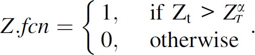
As in PAQ and EXP schemes, Z.fcn evaluates the error between the real and the predicted values. However, in the TS-SOUND case, the calculations of the predicted values are based on a time series model updated at each new sensor reading.

If Z.fcn = 1, the nodes opens a monitoring window and, for T time periods, sense and store the data. At time period t + T, the node evaluates two functions, Zb.fcn and Za.fcn, defined as following

$$\text{Zb}.\text{fcn}=\{\begin{array}{ll}1,& \text{if}\hspace{0.17em}{Z}_{t+T}^B\ge Z_T^{\alpha }\\ 0,& \text{otherwise}\end{array}\text{and}\text{Za}.\text{fcn}=\{\begin{array}{ll}1,& \text{if}\hspace{0.17em}{Z}_{t+T}^A\le Z_T^{c\cdot \alpha }\\ 0,& \text{otherwise}\end{array},$$

(20)

where $Z_{t+T}^B$ and $Z_{t+T}^A$ are defined by the expressions (15) and (16), respectively. The functions Z.fcn, Zb.fcn, and Za.fcn play the role of the g function in the data suppression framework in [1].

To decide if a message has to be sent to the base station, the node uses the following encoder function

$$f_{\text{enc}}=\{\begin{array}{ll}{\tilde{x}}_T,& \text{if}\hspace{0.17em}(Zb.fcn\cap Za.fcn)\\ \perp ,& \text{otherwise}\end{array},$$

(21)

where ${\tilde{x}}_T$ is the median of the T values read inside the post-monitoring window. If $T=1,{\tilde{x}}_1=x_{t+1}$ .

At each time period t, the base station waits for the r_t messages from the nodes and uses the following decoding function to update its database

$${\hat{x}}_t=\{\begin{array}{ll}{\tilde{x}}_T,& \text{if}\hspace{0.17em}{r}_t={\tilde{x}}_T\\ {\hat{x}}_{(t-1)},& \text{if}\hspace{0.17em}{r}_t=\perp \end{array}.$$

(22)

In case of data suppression (r_t = ⊥), the base station uses the last sent value, ${\hat{x}}_{(t-1)}$ , as the estimative for the current time period. Then, as we see in Eq. (22), the base station stores a sequence of median values.

The VB and the TS-SOUND schemes have similar encoding and decoding functions. They send only one value to the base station.

5.5. On TS-SOUND's Parameters

The TS-SOUND scheme is defined by three parameters: the size of the time windows (T); the amount of change in the expected behavior of the monitored variable we want to detect (α), and how much weight the current observation must have in the on-line updating of the distribution parameters (r).

As the length of the post-monitoring, the value of T should be as large as the size of the clusters of the aberrant readings. On the other hand, we should choose a small value for T to decrease the delays to detect an outlier and to update the base station if a change-point occurs.

As we will discuss in Section 7, we do not know how large the clusters of aberrant readings will be. Then, the choice of the value for T must consider the TS-SOUND's performance when it is applied on the time series with the clusters of aberrant readings of several sizes. Then, we have to choose the value of T that produces the most homogeneous performances considering aberrant clusters of different sizes. The experiments results in Section 7 will help us to make this choice.

On choosing the value of r, we should consider how large the local variation of the time series is. For instance, a wind speed time series has a local variation larger than the local variation of an atmospheric pressure time series (Fig. 4, Section 6). Therefore, the current observation in a wind speed series should have a weight (r) larger than the weight of the current observation in an atmospheric pressure series. However, giving larger weights to the observation in the estimation of the distribution parameters makes harder to detect this observation as an outlier. In fact, as we will see in Section 7, the values for r larger than 0.1 have degraded the suppression rates in the evaluation experiments.

Figure 4.

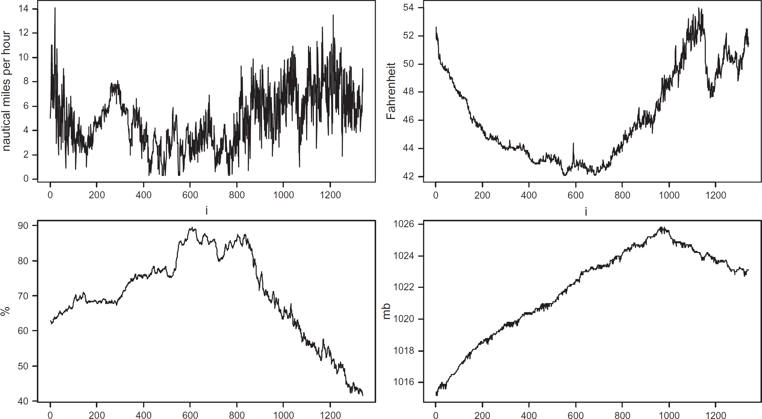
Typical daily time series used in the evaluation experiments. From left to right: wind speed (July'07); air temperature (April'06); air relative humidity (October'06); atmospheric pressure (April'07).

The value of α is the probability of making a mistake: detecting a non-outlier as an outlier. If we set a small value for α, we decrease this error probability. However, small values for α make harder the detection of change-points, especially if these points represent a small change in the expected behavior of the time series. On the other hand, if α is large, the scheme will be able to detect small changes, even though false outlier alarms will rise more often. Then, the user has to define what is more important to her, capturing small changes or avoiding aberrant readings.

6. Evaluation Experiments

In this section, we describe a set of extensive experiments to evaluate the performance of the TS-SOUND suppression scheme.

6.1. The Data

We used real data collected by the weather station of the University of Washington (USA) [22]. Our goal has been to be able to evaluate the performance of the TS-SOUND scheme and compare it with other suppression schemes considering data with diverse types of temporal behavior. Then, we have selected time series for wind speed (nautical miles per hour), air temperature (F), air relative humidity (%), and atmospheric pressure (milibars). The temporal resolution is one measurement per minute (average of measurements at each 5 seconds). To account for seasonal variability in the weather data, we have chosen four different months (October'06, January'07, April'07, and July'07). For each month, we have selected the data of the days from the 10^th to the 16^th. We have run the experiments using these 28 daily time series (1440 readings per series) for each variable.

Figure 4 presents the typical daily time series for each variable. These time series present different behaviors—from series with large local movements relative to its global variation (wind speed) until series with small local movements relative to its global variation (atmospheric pressure).

6.2. The Experiments

We have designed the experiments to evaluate the performance of the TS-SOUND scheme and compare it with the performance of the following suppression schemes: value-based (VB), exponential regression (EXP), and PAQ.

For the parameters of the TS-SOUND scheme, we have set the values r = (0.001, 0.005, 0.01, 0.05, 0.1, 0.2, 0.3, 0.4, 0.5, 0.6), α = (0.25, 0.20, 0.15, 0.10, 0.05, 0.025, 0.01) and T = (2, 4, 6, 8, 10). The value for the threshold $Z_T^{c\cdot \alpha }$ corresponds to the percentile 100(1 - cα/2) of the Gaussian distribution with mean zero and standard deviation √T. As we mentioned in section 4.2.2, we have adopted c = 1 in the threshold for $Z_{t+T}^B$ and c = 0.05 in the threshold for $Z_{t+T}^A$ . The first (100 + T) values of the time series have composed the learning sample.

Making the TS-SOUND scheme comparable to the other evaluated schemes (PAQ, EXP, and VB) is not a trivial task, since they use different criteria to trigger their data sending. The latter schemes use the absolute value of the prediction error to decide when the node must send data to the base station, whereas the TS-SOUND uses the detection/classification of outliers. Then, we have had to answer the question: “how to choose values for ε_υ and ε_VB (PAQ/EXP and VB error thresholds, respectively) so that we make these schemes comparable to the TS-SOUND scheme using the values chosen for α?”

Our solution for this problem has been to use the prediction errors of the TS-SOUND scheme to define the values for ε_υ and ε_VB . Then, after applying the TS-SOUND scheme to a real time series data using a given value for α, we have calculated the absolute prediction error as following

$$A{E}_t=|x_t-{\hat{x}}_t|,t=1,2,\dots ,N_{TS}$$

(23)

where ${\hat{x}}_t$ is the prediction value for real data x_t and N_TS is the size of the time series. To avoid the influence of discrepant values, we have decided to throw out the 10% largest values of AE_t and define the value for ε_υ and ε_VB as the percentile 90 of the AE_t values. Therefore, the maximum error of the predictions using PAQ, EXP, and VB schemes is the percentile 90 of the prediction error of TS-SOUND schemes. Once the range of the absolute prediction error has been equalized, the distribution of the error within this range will be determined by the performance of the evaluated schemes.

The values for the other parameters of PAQ and EXP have been chosen based on the values cited in [4] as good choices : ε_δ = (1.8/3.0)ε_υ, A_PAQ = (5, 15) and a = (8/15)A_PAQ. The learning sample size (N_LS) has been set as the first 100 observations of the time series.

6.2.1. Evaluating the Influence of Aberrant Readings

We have designed an experiment to evaluate how sensitive to aberrant points are the suppression schemes analyzed in this article. This experiment has used using the real time series previously described. For each time series, we have inserted aberrant values, isolated or clustered, in randomly chosen time periods. To generate isolated aberrant readings, we have sampled 100 time periods of a given time series to be replaced by an aberrant reading, preserving a minimum interval of 11 time periods between two sequential positions. Then, about 10% of a time series has been composed by aberrant points. To generate the aberrant reading at the selected time period, we have used the interquartile range IQ, defined as IQ = P_diff(75) - P_diff(25), where P_diff(p) is the percentile p of the sequential differences |X_t - X_t−1|. In a boxplot analysis [21], values smaller than P_diff(25) − 3 x IQ or greater than P_diff(75) + 3 x IQ are considered to be extreme outliers. Then, to generate an aberrant reading, we have added (sign x range x IQ) to the current value of the candidate time period, where range has been randomly chosen inside the interval [3; 6] and sign has been randomly chosen between −1 and +1. Adopting the boxplot's rule and a random value for range, we have expected to decrease our influence on the generation of the aberrant values.

In addition to isolated aberrant readings, we have generated clusters with 2, 3, 4, and 5 aberrant readings. From now on, we will denote the clusters of the aberrant readings by aberrant clusters. To produce such clusters, we have supposed that all the aberrant readings in a cluster are generated in the same direction, as those presented in Fig. 1. Given the size of the cluster, we have grouped the initial 100 aberrant readings. For instance, in the experiments with clusters of 4 aberrant points, we have generated 25 clusters. The first reading of the cluster has been inserted in the time series as in the isolated case. To generate the sequential aberrant readings, we have used the same rule to produce the first aberrant reading. However, their signs have been constrained to the sign of the first reading in the cluster. We have applied the TS-SOUND, PAQ, EXP, and VB schemes on these modified time series using as parameters the values described in the previous section.

6.2.2. Assessing the Performance of the Suppression Schemes

We have evaluated the performance of suppression schemes using the trade-off between two measures: the suppression rate and the prediction error.

We have adopted the median absolute error (MAE) to measure the prediction error. The median absolute error has been calculated as

$$MAE=media{n}_{(t-1,2,\dots ,N_{TS})}|X_t-{\hat{x}}_t|,$$

(24)

where N_TS is the size of the time series.

We can cite some advantages of adopting MAE to assess the prediction error instead of using other error measures such as the mean square error (MSE). First, the absolute difference between the predicted and the real values is an intuitive measure for the prediction error. Second, the absolute error preserves the original measurements units, which makes its interpretation easier. Finally, the median is more robust to the influence of discrepant values.

The suppression rate (SR) has been calculated as the proportion of suppressed data

$$\text{SR}=1-\frac{(\text{number of sent messages})}{N_{TS}}.$$

(25)

If a scheme increases its suppression rate, we expect MAE also increases, since the node updates the base station database less often. A suppression scheme S1 can be defined as better than other suppression scheme S2 if, for a given value of prediction error, S1 is able to get suppression rates larger than the suppression rates of S2.

To evaluate the robustness to aberrant readings of the TS-SOUND scheme, we have calculated the odds of sending data to the base station provided that an aberrant reading has been detected as

$$Odd{s}_{SENT}^{Aberrant}=\frac{\text{number of detected aberrant readings that have caused data sending}}{\text{number of detected aberrant readings that have not caused data sending}}.$$

(26)

A TS-SOUND scheme is considered to be robust to aberrant readings if its $Odd{s}_{SENT}^{Aberrant}$ is smaller than 1. Then, a suppression scheme S1 can be defined as more robust to aberrant readings than a suppression scheme S2 if S1 has got an odds of sending data smaller than S2's odds.

Since PAQ, EXP, and VB schemes always send the detected outliers to the base station, their $Odd{s}_{SENT}^{Aberrant}$ are infinite. Then, we have evaluated the robustness to aberrant readings of these schemes by comparing their suppression rates in the time series with and without aberrant readings. For a robust scheme, this ratio is close to 1.

7. The Results

In this section, we present the main results of the extensive experiments described in the previous section. We start our analysis with a simple case study.

7.1. A Simple Case Study

We have had access to the air temperature and relative humidity data collected by three Tmote Sky sensor nodes ² . They have collected data at each 30 s during 32 h. Each sensor node has produced about 4000 readings of each variable. The left side of Fig. 5 presents the time plot of the temperature data collected by the sensor node 2.

Figure 5.

Results of TS-SOUND scheme: time series predicted at the base station (on the right); real air temperature data collected at the sensor node 2 (on the left).

Since these data do have not enough time series to be used in an extensive evaluation, we have used them to perform an initial analysis. Table 1 presents the values for the performance measures of the evaluated schemes using T = 2, α = 0.15, r = 0.1 (TS-SOUND's parameters) and A_PAQ = 15 (PAQ and EXP's parameter). The values for ε_υ and ε_VB were determined as we have described in section 6.2.

Table 1

Results of the evaluation experiments applied to the air temperature (°C) and relative humidity (%) data collected by three Tmote Sky sensors: suppression rate and median absolute error (within the parenthesis)

Scheme	Sensor Node 1		Sensor Node 2		Sensor Node 3
	Temperature (ευ = εVB = 0.03°C)	Relative Humidity (ευ = εVB= 0.41%)	Temperature (ευ = εVB = 0.08°C)	Relative Humidity (ευ = εVB = 0.25%)	Temperature (ευ = εVB= 0.03°C)	Relative Humidity (ευ= εVB = 0.17%)
TS-SOUND	0.823	0.857	0.858	0.877	0.865	0.883
(r = 0.1;T = 2; α = 0.15)	(0.005°C)	(0.057%)	(0.015°C)	(0.040%)	(0.010°C)	(0.020%)
PAQ	0.753	0.807	0.812	0.826	0.783	0.836
(APAQ = 15)	(0.014°C)	(0.157%)	(0.031°C)	(0.086%)	(0.010°C)	(0.053%)
EXP	0.893	0.816	0.825	0.829	0.789	0.846
(APAQ = 15)	(0.010°C)	(0.146%)	(0.028°C)	(0.082%)	(0.009°C)	(0.051%)
VB	0.858	0.872	0.874	0.892	0.859	0.897
	(0.010°C)	(0.124%)	(0.020°C)	(0.086%)	(0.010°C)	(0.041%)

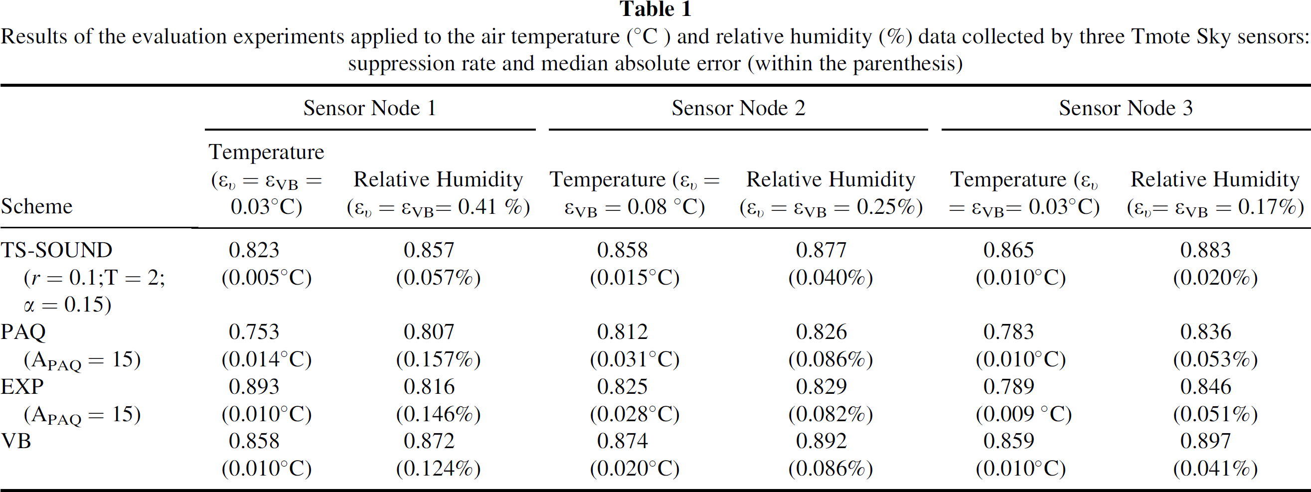
For both variables, the TS-SOUND has got suppression rates similar to the rates of the other schemes, whereas its prediction error has been smaller than the prediction error of the other schemes. The right side of Fig. 5 presents the time series predicted at the base station when the TS-SOUND scheme has been applied to the temperature data collected by the sensor node 2. Comparing the real and predicted series, we have noticed that the TS-SOUND avoids reporting the erratic movement of the series as, for instance, in the beginning and final parts of the time series in Fig. 5. On the one hand, the TS-SOUND delays the notification of fast changes such as the one near the time period 2000. The TS-SOUND classifies this behavior as an aberrant one until it notices there is a change. From this moment on, it updates the base station more often. On the other hand, likely clusters of aberrant readings are represented by few updates, as those ones near the time period 3000.

Since no messages can be sent to the base station during the TS-SOUND's monitoring window, increasing its size (T) has increased the suppression rates. As a result, the value of the median absolute error has also increased. The parameter α has had a similar effect on the suppression rates and prediction errors: the larger the rigor to consider an observation as an outlier, the larger the chance of suppressing data.

On the value of r, our initial experiments have pointed to r = 0.1 as the value that produces the best trade-off between the suppression rate and the prediction error. This means that we obtain the best performance for the TS-SOUND when the on-line estimation of the new values for the distribution parameters sets less weight to the current sensor reading (Eqs. (7–11)). The TS-SOUND schemes using r values smaller than 0.1 have produced results very similar to the results with r = 0.1. However, increasing the value of r up to 0.5 has degraded the suppression rates. In fact, giving larger weights to the observation in the estimation of the distribution parameters makes it harder to detect this observation as an outlier.

7.2. Selecting the Best Value for the Length of the Monitoring Window

The TS-SOUND's strategy to distinguish a change-point from an aberrant reading is to use a post-monitoring window whenever an outlier is detected. This time window works as a filter of aberrant readings and makes the TS-SOUND robust to these erroneous data. The success of this filtering strategy is closely related to the length of the monitoring window. We expect large aberrant clusters require large windows to be filtered. However, we do not know how large the clusters of the aberrant readings will be.

In this section, we examine the results of experiments with the meteorological data of the University of Washington to answer the following question: “Considering several sizes for the clusters of aberrant readings, which is the minimum value for the length of the monitoring window that leads to the TS-SOUND scheme with

the largest robustness to aberrant readings and

the best trade-off between suppression rate and prediction error ?”

To answer the first part of the question, we have summarized some of the experiments' results using plots as the ones in Fig. 6. They present the odds of “sending data to the base station provided that an aberrant reading has been detected” as a function of the length of the monitoring window considering aberrant clusters of several sizes. Figure 6 presents the results for the sets of time series that have got the most irregular behaviors: air relative humidity and wind speed measurements. We have looked for the smallest length for the monitoring window that leads to the most similar values for the odds among aberrant clusters of different sizes. For the wind speed time series, the monitoring windows of length 10 and 2 have presented the most similar odds. Then, the chosen length is T = 2. For the air relative humidity, the length is also T = 2. For air temperature and atmospheric pressure time series, the larger the monitoring window is, the less homogeneous the odds are. Therefore, T = 2 is the chosen length.

Figure 6.

Robustness to aberrant readings of TS-SOUND scheme according to the length of the monitoring window (T) and the size of the aberrant clusters (CS). The other TS-SOUND's parameters have been α = 0.15 and r = 0.1.

Increasing the value of α decreases the odds of “sending data to the base station provided that an aberrant reading has been detected,” since the rigor to classify an observation as an outlier increases.

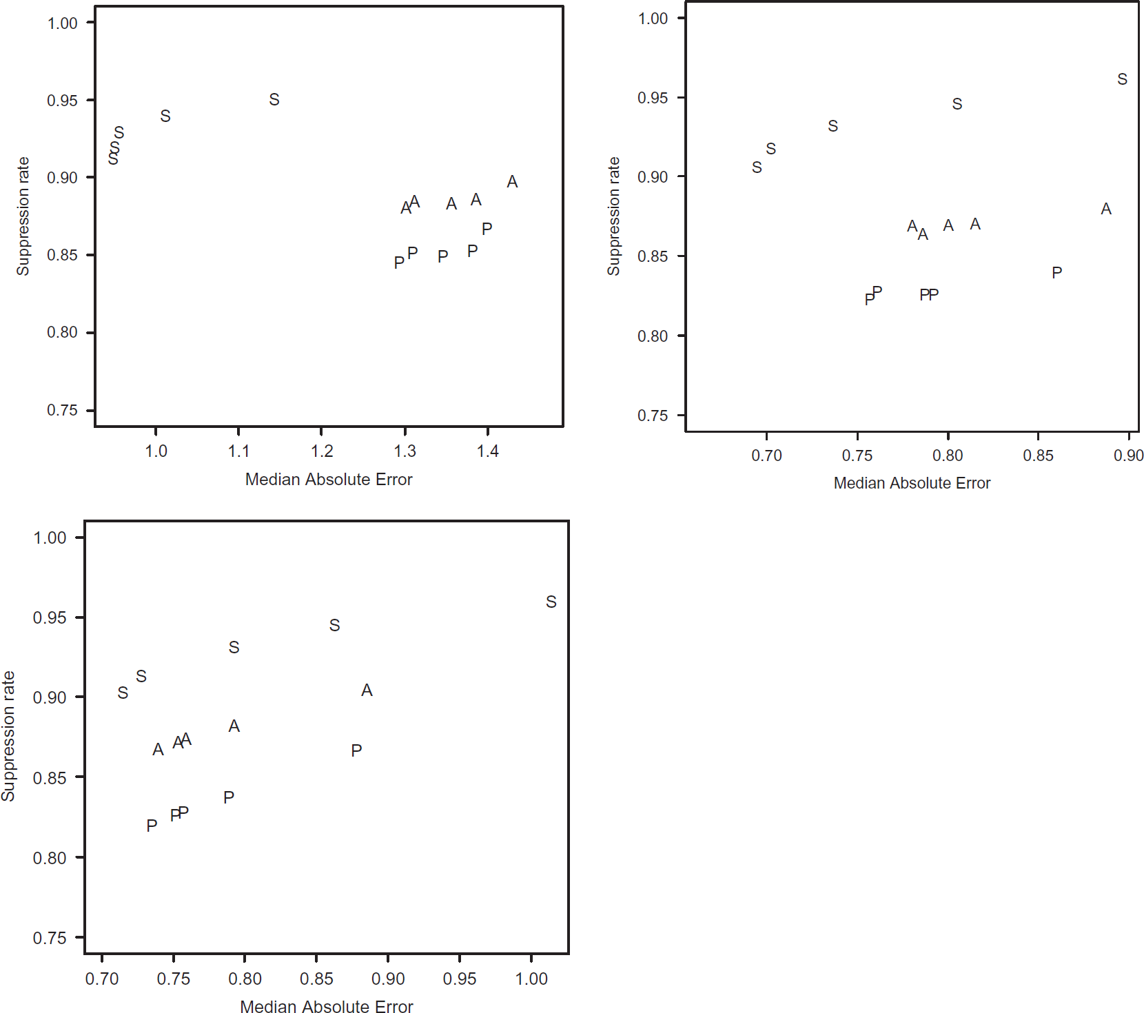
We have answered the second part of the question by examining plots as the ones in Fig. 7. They present the trade-off between the suppression rate and the prediction error for several lengths of the monitoring window and considering the aberrant cluster of different sizes. We have looked for the smallest length for the monitoring window that leads to the most similar suppression rates and prediction errors among aberrant clusters of different sizes. For wind speed and air relative humidity time series (Fig. 7), we have looked for the group of symbols (T values) that are more “clustered.” The monitoring windows of length 6 and 4 have presented the most similar suppression rates and prediction errors. Then, the chosen length is T = 4. Examining the air temperature and atmospheric pressure time series, we have got the same value for T.

Figure 7.

Performance of TS-SOUND scheme applied to wind speed and air relative humidity time series. The parameters have been α = 0.15, r = 0.1 and several values for the length of the monitoring window (T). Each point represents the summary of the results for time series with aberrant clusters of different sizes: 1 (isolated aberrant readings), 2, 3, 4 and 5.

Since we have got different answers for the two parts of the proposed question, we have chosen the best value for T by examining the effect of using the value chosen in part (a) on the context of part (b) and vice versa. Then, we have examined the effect of choosing T = 2 on the trade-off between the suppression rate and the prediction error and the effect of using T = 4 on the odds of “sending data to the base station provided that an aberrant reading has been detected.” In the former case, exchanging T = 4 for T = 2 produces a substantial increasing in the heterogeneity of the suppression rates and prediction errors for the wind speed, air temperature, and atmospheric pressure time series. In the latter case, the effect of exchanging the values of T (T = 2 for T = 4) is smaller than in the former case. The worst effect has occurred in the air relative humidity time series (right side of Fig. 6). For T = 4, the odds of “sending data to the base station provided that an aberrant reading has been detected” is, in median, equal to 1 when isolated aberrant readings (CS = 1) occur in the time series. However, the other odds are smaller than 1. Then, considering all evaluated time series and sizes for aberrant clusters, we have chosen the value 4 as the best one for the length of the monitoring window.

7.3. Evaluating the Schemes' Performances

In this section, we compare the performance of TS-SOUND scheme using T = 4, selected in the previous section, with the performance of the PAQ, EXP, and VB schemes.

As we have mentioned in Section 6, we have used the trade-off between the suppression rate and the prediction error of a scheme as a measure for its performance. We represent graphically this trade-off for each one of the sets of meteorological time series using the scatter plots of the figures from 8a to 8d. Each point of a scheme represents the summary of its performance using a different value for α (0.15, 0.10, 0.05, 0.025, 0.01), in this order, following the increasing of the suppression rates. For PAQ/EXP and VB schemes, the values for the correspondent error thresholds ε_δ and ε_VB, respectively, have been defined as described in Section 6.2. Points closer to the upper-left corner represent the schemes with the best performances. Since TS-SOUND with T = 4 has got its worst results when the times series had isolated aberrant readings (Figs. 6 and 7), we have chosen to use this scenario to compare TS-SOUND's performance with the performance of the other evaluated schemes. The upper and bottom subfigures illustrate which data the base station would have if the node applied the TS-SOUND and VB schemes, respectively, on the real times series in the middle subfigure. The real times series in the middle subfigures are the original ones in Fig. 4 with generated aberrant clusters of size 1 (isolated aberrant readings).

To understand what values we should expect for the prediction errors so that we could consider them acceptable, we have used the size of the sequential changes in the time series as a basis for comparison. Then, we have calculated the sequential absolute differences, |X_t - X_t-1|, in the series of each variable and summarized the sequential changes (non-zero differences) using the percentiles 5 and 95. Therefore, in the air relative humidity and temperature time series, 90% of the sequential changes are within the interval [0.10; 1.0]% and [0.10; 1.0] F, respectively. In the atmospheric pressure time series, 90% of the sequential changes are within the interval [0.10; 0.40] mb. In the wind speed time series, 90% of the sequential changes are within the interval [0.10; 2.1] nautical miles. Analyzing the figures from 8a to 8d, we notice that all evaluated schemes have got median prediction errors compatible with the expected sequential changes in a given type of meteorological time series. In other words, all evaluated schemes have got acceptable errors on predicting the real time series at the base station.

Figure 8.

(a) Performance of the evaluated schemes in the air relative humidity times series with isolated aberrant readings. Legend: S for TS-SOUND (r = 0.1, T = 4), V for value-based, P for PAQ (A_PAQ = 15) and E for EXP (A_PAQ = 15). Each point of a scheme represents the summary of its performance using a different value for α (0.15, 0.10, 0.05, 0.025, 0.01), in this order, following the increasing of the suppression rates. For PAQ/EXP and VB schemes, the values for the correspondent error thresholds ε_δ and ε_VB, respectively, have been defined as described in Section 6.2. (b) Performance of the evaluated schemes in the air temperature times series with isolated aberrant readings. The legend and other details are in the caption of Fig. 8a. (c) Performance of the evaluated schemes in the atmospheric pressure times series with isolated aberrant readings. The legend and other details are in the caption of Fig. 8a. (d) Performance of the evaluated schemes in the wind speed times series with isolated aberrant readings. The legend and other details are in the caption of Fig. 8a.

The TS-SOUND scheme has got its best performance in air relative humidity and temperature time series (Figs. 8a and 8b, respectively). In the air relative humidity data, the TS-SOUND has been the scheme with the best performance for all values of α, reaching the highest suppression rates and the smallest prediction errors. For the smallest two values of α in the air temperature data and for α = (0.10, 0.05) in the atmospheric pressure data (Fig. 8c), the prediction errors of the TS-SOUND and VB are, in median, the same. However, the TS-SOUND has got suppression rates higher than VB's rates.

In the wind speed time series, which have a large local variation, the TS-SOUND has increased the prediction errors in comparison to the other schemes' errors (Fig. 8d). Nevertheless, it has got a higher increase in the suppression rates in relation to maximum possible increasing. As an example, for α = 0.15, the TS-SOUND has got a median prediction error of 0.8 nautical miles per hour, which has been 14% larger than the VB's median prediction error. However, the TS-SOUND's suppression rate has been 0.938, whereas VB has got 0.798. Then, the TS-SOUND's rate has got an increasing of 69% in relation to maximum increasing in the VB rate (1 − 0.798). For α = 0.10, TS-SOUND's error has been 43% larger than VB's error but TS-SOUND's has increased the suppression rate in 77% of the maximum possible increasing. If we compare the TS-SOUND with the PAQ and EXP schemes, the gains are higher.

In the time series with small local variation, as the atmospheric pressure series, the VB scheme has got median prediction errors equal to zero, even suppressing about 77% of the readings (Fig. 8c). However, the correspondent TS-SOUND scheme has suppressed about 95% of the readings, in median, at the cost of increasing 0.05 milibars in the prediction error. Since this increasing is among the 5% smallest sequential changes in the atmospheric pressure series, we conclude it is worth adopting the TS-SOUND for this type of data, getting a higher suppression rate at the cost of a small increasing in the prediction error.

On choosing the best value for α, we have to consider how large the local variations in the series are. Comparing Figs. 8c, a, b, and d in this order, we conclude the larger the local variation the larger the best value for α must be. In general, for values of α larger than 0.05, the increasing in the suppression rate does not compensate the increasing in the prediction error.

Comparing the predicted time series to the real ones (subfigures), we notice the robustness to the aberrant readings of TS-SOUND scheme, whereas VB suffers a large influence of these erroneous data. VB's predicted series are similar to the series with aberrant readings (middle subfigures), whereas TS-SOUND's predicted series look like the original series, without aberrant readings, in Fig. 4.

PAQ and EXP schemes using the largest monitoring window (A_PAQ = 15) have got suppression rates larger than the rates of those schemes using a smaller window (A_PAQ = 5). Therefore, PAQ and EXP schemes having a larger period to evaluate the re-estimation of the model parameters have been a better alternative, even if the prediction errors have been slightly larger. Despite having updated the base station more often than the other schemes, the PAQ and EXP schemes have not got the smallest prediction errors. In other words, using these model-based suppression schemes is not a good strategy if the dataset may have aberrant readings.

7.4. Evaluating the Schemes' Robustness to Aberrant Clusters

In this section, we compare the robustness to aberrant clusters of the suppression schemes. Since the $Odd{s}_{SENT}^{Aberrant}$ of PAQ, EXP, and VB are infinite, we have calculated the ratio between the suppression rates with and without aberrant clusters. A suppression scheme robust to aberrant readings should present this ratio close to 1. For a suppression scheme that suffers the influence of aberrant readings, this ratio is smaller than 1.

Figure 9 presents the ratios for the suppression schemes applied on atmospheric pressure and wind speed time series. In these sets of series, the evaluated schemes have suffered the largest and the smallest influence of aberrant clusters, respectively.

Figure 9.

Influence of aberrant readings on the suppression rate of the evaluated schemes applied on atmospheric pressure and wind speed time series. Legend: S for TS-SOUND (r = 0.1, T = 4, α = 0.15), V for value-based, P for PAQ (A = 15) and E for EXP (A = 15).

The suppression rates of the TS-SOUND scheme have not presented relevant changes, whereas the suppression rates of the other schemes have decreased, especially for the PAQ and EXP schemes. This is because the model-based prediction adopted by the PAQ/EXP schemes is quite sensitive to the aberrant readings. They decrease PAQ/EXP's suppression rates for two reasons: the node has to send them as detected outliers to the base station and they cause the re-estimation (and sending) of the new model parameters.

For the VB scheme, aberrant clusters make nodes send data to the base station at least two times: in the beginning and in the end of the cluster. Inside the cluster, aberrant readings tend to be similar to each other. This reduces data sending. This could explain why the influence of the aberrant readings on the suppression rates has been smaller for aberrant clusters than for isolated aberrant readings. Clusters of aberrant readings would tend to amortize the initial and final data sending.

7.5. A Note on the Order of the AR Model

The model-driven approach is an efficient solution to data collection in sensor networks if the monitored variable has a well-known behavior so reliable models can be defined [1]. Then, let us suppose that a sophisticated model is the best representation for the expected behavior of the sensor data. In this case, the simplicity of AR(1) model in the TS-SOUND scheme could degrade its performance if we compare it to the performance of a scheme adopting a more sophisticated model.

To evaluate this hypothesis, we have simulated time series according to the AR(3) model, which is the model that the PAQ scheme uses. To generate the model coefficients, we have fit an AR(3) model to the time series in Fig. 4, which represents the typical time series for each variable we have considered in the experiments. For each set of coefficients, we have simulated 50 time series with 1440 observations each, which corresponds to 50 days of monitoring with one reading per minute).

The simulated time series have presented different behaviors because the AR(3) coefficients used in the simulations have come from series with different behaviors (Fig. 4). Since it is necessary to analyze the schemes' performances in groups of series with similar behaviors, we have had to quantify the differences between the behaviors of the simulated time series. To do this, we have defined the Relative Lagged Difference (RLD _l ) as

$$RL{D}_l=\frac{\underset{t=l+1,l+2,\cdots ,N}{median}(|X_t-X_{t-l}|)}{\underset{t=1,\cdots ,N}{max(X_t)}-min(X_t{)}_{t=1,\cdots ,N}},l=1,2,\cdots ,N-1.$$

(27)

It compares the typical (median) difference between time periods t and t-l with the total range of the values. The values of RLD _l range from 0 to 1. The lag l indicates how local is the movement we want to capture. The smaller the value of l, the more localized the analysis. For instance, the values of RLD₁₀ for the time series in Fig. 4 are: 0.0942 (wind speed), 0.0252 (air temperature), 0.0201 (air relative humidity), and 0.0081 (atmospheric pressure). Therefore, the time series with smoothe changes relative to the total range (e.g., atmospheric pressure) have low values for RLD _l , whereas abrupt changes result in a higher value for RLD _l (e.g., wind speed).

After calculating the RLD₁₀ for all 200 times series, we have separated them into three groups according to their RLD₁₀ value and applied the TS-SOUND and PAQ schemes on the time series of each group. The values for the parameters have been the same of the experiments in Section 7.4.

Figure 10 presents the summaries for the performance of both schemes in the three groups of the time series. Similarly to the figures of Section 7.1, points closer to the upper-left corner represent the schemes with the best performances. As in the experiments with real data, the PAQ scheme using the largest post-monitoring window (A_PAQ = 15) have outperformed the schemes using a smaller time window (A_PAQ = 5).

Figure 10.

Summaries for the performance of TS-SOUND and PAQ schemes in data simulated according to the AR(3) model. Legend: S for TS-SOUND (r = 0.1, T = 4), P and A for PAQ with A_PAQ = 5 and 15, respectively. Each point of a scheme represents the summary of its performance using a different value for α (0.15, 0.10, 0.05, 0.025, 0.01), in this order, following the increasing of the suppression rates. For PAQ scheme, the values for the correspondent error thresholds, ε_δ, have been defined as described in section 6.2. (a) 0 < RLD₁₀ < 0.025; (b) 0.025 ≤ RLD₁₀ < 0.05; (c) 0.05 ≤ RLD₁₀ < 0.075.

We expected that the PAQ scheme could get at least prediction errors smaller than the errors of the TS-SOUND. However, even in a scenario clearly favorable to PAQ, the most of TS-SOUND schemes have outperformed their correspondent PAQ schemes. In the time series with smooth changes relative to the total range (Fig. 10a), all the TS-SOUND schemes have outperformed all the PAQ schemes, getting the highest suppression rates and the smallest prediction errors. As the time series have increased their local variation relative to their total range (RLD₁₀ increases), the PAQ schemes have got prediction errors closer to the errors of the TS-SOUND schemes. However, for the first two values of α, the TS-SOUND has still outperformed PAQ.

8. Discussion

Data suppression schemes are defined by an agreement between the sensor nodes and the base station about the expected behavior for the sensor readings. To decide when the sensor nodes may suppress their data, the schemes evaluate the prediction error, which is the difference between the value the sensor actually collects and the value predicted according to the expected behavior for the sensor readings. If the collected value fits the expected behavior, the node suppresses its data. Otherwise, it sends data to the base station.

Since the schemes for data suppression look for changes in the expected behavior of the sensor data, they are sensitive to aberrant readings. Transmitting these erroneous data is a waste of energy. In a simple suppression scheme as the Value-based [1], for instance, an aberrant point may produce two unnecessary messages to the base station. That is because the scheme detects two sequential changes of behavior, one when the aberrant readings occur and another when the readings get normal again.

To avoid sending aberrant readings, one can propose to use a fixed threshold—readings smaller or greater than a predefined value would be considered as erroneous data. However, that is a naive solution, since what would be aberrant at a time period of the series might not be aberrant at another time period. For instance, a reading of 1026 mb at time period 200 in the atmospheric pressure series (Fig. 4) would be considered aberrant. However, this value should not be considered aberrant at time period 1000.

In this article, we have proposed the TS-SOUND, a scheme for temporal data suppression in sensor networks that is robust to aberrant readings. The TS-SOUND considers the data collected by a sensor node as a time series and monitors the behavior of this series. It adopts a procedure to detect outliers from a time series and the posterior classification of the detected outlier into change-points or aberrant readings. In the former case, data are sent to the base station, since it means a change in the expected behavior of the data series. Otherwise, data are suppressed.

Schemes for temporal data suppression proposed in sensor networks literature (PAQ [4], EXP, and Value-based [1]) suppress data by comparing the absolute value of the prediction error with a fixed threshold. Using the absolute value of the prediction error allows for controlling its maximum value. However, if the random fluctuations around the expected value (local variations) are larger than the threshold for the absolute error, a large amount of unnecessary data will be sent to the base station and the suppression rates will be small. On the other hand, if the local variations are smaller than the threshold for the absolute error, the suppression scheme will not be able to capture changes in the expected behavior of the monitored data. Then, if the time series has a nonstationary variance, a fixed threshold for the absolute prediction error will not be able to work well during all data collection.

The TS-SOUND scheme also uses an error measure to decide if an observation is an outlier. However, it adopts a relative error measure, comparing the absolute error with the data variance, which captures the random fluctuations of the data. As a result, the TS-SOUND is able to be adaptable to the local variations of the time series. The suppression rates of the TS-SOUND scheme are more robust to the size of the local variations than the other schemes evaluated in this article.

Besides adopting the relative prediction error, the TS-SOUND scheme tries to minimize its sensitivity to aberrant readings using the past data through a moving average. Moreover, even if an aberrant reading raises the outlier alarm, the TS-SOUND opens a post-monitoring window to avoid sending this erroneous data to the base station. Although this post-monitoring window introduces a delay in the data delivery, our experiments have shown that a small delay (four time periods) can deal with time series presenting aberrant clusters of several sizes.

Using real data from several sources and presenting different temporal behaviors, we have run experiments to evaluate the suppression rates of the TS-SOUND scheme and the prediction errors attached to them. We have used both of these measures to quantify the performance of a data suppression scheme. We have also evaluated TS-SOUND's robustness to aberrant readings and compared its performance with the performance of PAQ, EXP, and VB schemes. The evaluation experiments have shown that the TS-SOUND is more robust to aberrant readings than the other schemes considered in this article. Moreover, the TS-SOUND has outperformed the model-based suppression schemes (PAQ and EXP) in all evaluated scenarios and the VB scheme in the most of these situations.

Value-Based is the simplest suppression scheme and has got one of the best performances in our experiments. However, we can list at least three situations in which using the TS-SOUND would be better than using the Value-Based scheme:

when the applications are not interested in aberrant readings;

when the series presents different behaviors along the time, since VB uses a fixed error threshold and the TS-SOUND is adaptable to the local variation of the time series;

when having high suppression rates is more important than having small prediction errors.

To define a TS-SOUND suppression scheme, the user has to choose the values for three parameters: the weight of the last sensed data (r) in the on-line estimation of the distribution parameters, the length of the post-monitoring and past time windows (T), and the rigor to classify an observation as an outlier (α). As we have discussed in Section 7, we have found that the value of T has not to be as large as the cluster size. Our experiments have pointed out to 4 as the smallest value for T that leads to homogeneous performances in time series with different behaviors and several sizes of aberrant clusters. On the value of r, our experiments have shown that we obtain the best performance for the TS-SOUND when the on-line estimation of the new values for the distribution parameters sets less weight to the current sensor reading. TS-SOUND schemes using r = 0.1 have produced the best results and values of r smaller than 0.1 have got very similar results. However, weights larger than 0.1 have degraded the suppression rates.

Since the values for T and r can be constrained to some predefined values, the network user has to choose only the value for α. To do this, it is necessary to define what is more crucial, capturing small changes (large values for α) or avoid aberrant readings (small values for α).

The main contributions of this article are twofold: a proposal for a data suppression scheme that is robust to aberrant readings and the evaluation of the performance of data suppression schemes considering not only the saved energy but also the quality of the data collected at the base station.

9. Future Directions

Sensor networks collect spatially correlated data, which produces areas in the sensors field that are spatially homogeneous. Our future work includes a spatio-temporal version of the TS-SOUND scheme having as its spatial basis the clustering algorithm in [23]. Instead of sending its reports to the base station, the nodes organize themselves into clusters that explore the spatial homogeneity of the data in the sensors field. Besides localizing the most part of the communication among the nodes, such clusters improve the quality of the cluster data summaries to be sent to the base station [24].

The nodes of a sensor network are prone to failures as well as the communication between nodes can be very noisy. Thus, a data collection protocol based on a suppression scheme has to address an important question: how can we distinguish suppressed reports from nodes failures and lack of communication between the nodes and the base station? Silberstein et al. [25] have proposed interesting alternatives to deal with this problem using Bayesian inference. We study to incorporate the proposed solutions in the spatio-temporal version of the TS-SOUND scheme.