Sage Journals: Discover world-class research

Abstract

Compared with the small overhead of data payload in sensor networks, the overhead of MAC address is significant from the point of view of energy-saving. A distributed algorithm (Virtual Grid Spatial Reusing-VGSR) for MAC address assignment is presented in this paper, which is a low energy cost algorithm and reduces the size of the fixed MAC address largely based on the mapping of the geographical position. Moreover, VGSR algorithm scales well with the network size and achieves the optimum performance by adjusting the communication range of sensor nodes. In typical scenarios, the MAC address size is 5 bits and the corresponding average size is only 3.86 bits, which outperforms other existing approaches.

1. Introduction

With the development of the wireless communication and micro-elector-mechanism-system, the low-cost, low-power, multifunctional sensor nodes have emerged in recent years [1]. Wireless sensor network that is made up of these nodes is a new technology of acquiring and processing information. It is widely applied in both military and civil fields and is becoming the focus of many researchers.

Large scale is one of the most obvious features of the sensor network. Thousands or even millions of these nodes work together in an Ad Hoc fashion and constitute a highly distributed system. The sheer number of these nodes makes centralized algorithms requiring global communication unacceptable. The network must apply distributed algorithms instead to avoid network-wide communication and coordination.

Sensor nodes are typically small in size, usually as tiny as a coin [1]. Such a small size can enhance the flexibility of sensor nodes, but one of the disadvantages is that the limited energy reserve on each node restricts the lifetime of the sensor network severely. Considering that the power recharge is impossible actually, every senor node must operate in an energy-efficient way. It is evident that the transmission of every bit will consume corresponding energy [2]. Therefore, to maximize the lifetime of the system, it is crucial to minimize the number of the bits in the transmitted packet. The sharply reduced payload of data [2] makes the overhead of the header evident, so the energy consumed by MAC address occupies a relatively great proportion.

There have been many research works in the area of the MAC address assignment. In order to reduce the large address size Jeremy Elson and Deborah Estrin propose a Random, Ephemeral Transaction Identifiers (RETRI) [2]. Probabilistically unique identifiers are selected by nodes for each new transaction. RETRI scales with the network very well, but it could not resolve MAC address collisions, and will result in information loss, another form of energy waste.

Curt Schurgers et al. describe a MAC address assignment mechanism for sensor networks [3, 4]. All of the sensor nodes reuse the limited address spatially and the encoded address representation reduces the size of the MAC address ulteriorly. When the average connectivity is 10, the average address size achieves 4.41 bits. However, the variable address length requires extra processing cost and the periodic broadcasting between neighbor nodes also lead to great cost of the energy.

Muneeb Ali and Zartash Afzal Uzmi propose a node address naming scheme, which assigns locally unique addresses by spatial reusing for nodes in an energy efficient manner [5]. The focus of their work is on clustering network, whereas we mainly discuss the flat sensor network.

A. Dunkels et al. discuss an address constructing method called “spatial IP” [6], which uses the location of nodes to constitute an IP address. The energy consumption of the algorithm itself is low relatively, but the address size is very large. That can not meet the demand of energy conservation of the sensor network.

Different from the techniques above, we present a distributed algorithm Virtual Grid Spatial Reusing (VGSR), which assigns a local unique MAC address for sensor nodes efficiently. Basing on the feature that MAC address should be unique only in a local area, VGSR reuse MAC addresses with fixed size in space. Besides, VGSR enables the sensor node to get its MAC address by mapping from the geographical position and reduces the size of MAC address greatly. In typical scenario, the address requires 5 bits and the corresponding average size is only 3.86 bits. Owing to both the reduction of MAC address size and the full use of location information, VGSR results in significant energy savings, which translates directly into the extension of the lifetime of sensor nodes ultimately.

The remainder of this paper is organized as follows: Section II discusses the condition of MAC address reuse. In Section III, we describe the basic idea of VGSR. We simulate and analyze the performance of VGSR in Section IV. Finally, we conclude this paper in Section V.

2. Reuse Conditions

MAC address is the identifier of nodes on the data-link layer. From now on, we will use the term “address” to denote the MAC address. For convenience, the address in traditional networks is often the same as the net ID which is global unique [3]. The large size of the address leads to tremendous overhead. Thus it is unsuitable for sensor network.

Considering that the function of the address is to distinguish the sender and receiver at each hop, we can reuse them in different areas. A simple scenario in Fig. 1 shows how the reuse can be realized. Although node A and D have the same address “1”, no ambiguity of communication exists. The intuitive reason for this is that the distance between node A and node D is large enough such that they do not have a neighbor in common. For a more exact conclusion, we discuss the reuse condition further. Due to the identity of the wireless propagation environment, we just consider the bi-directional channel.

Figure 1.

MAC address reusing.

Each sender (receiver) should be able to uniquely identify a given receiver (sender). Therefore, neighbor nodes should have different addresses. We summarize these constrains as Condition 1.

Condition 1: For any node A, all its neighbors as well as A must have addresses different from each other.

When the distance between a pair of nodes is two hops, both of them must be the neighbors of a third node. According to Condition 1, they should have distinct addresses. This means that all nodes in the two-hop range of any node A must have different addresses from node A, while out of this range the address of node A can be reused. We summarize this as Condition 2.

Condition 2: The minimum reusing range must be larger than two-hop range.

3. VGSR Algorithm

VGSR is a distributed algorithm based on geographical position, which efficiently assigns local unique MAC addresses with a fixed size for sensor nodes. In VGSR, according to the network scale, each sensor node will first conceive a virtual grid including a series of virtual square cells for which spatially reused local unique identifiers are assigned. Secondly, every sensor node distributing randomly maps its geographical position coordinates onto a unique cell and chooses the identifier of the cell (cell address) as its MAC address. After declaration, sensor nodes can use the MAC address without conflict. In order to explain VGSR algorithm in more detail, we split the VGSR algorithm in four parts: the construction of virtual grid and cells, address assignment, mapping, and collision resolving. In what follows, we elaborate on each of them.

3.1. The Construction of Virtual Grid and Cells

After deployment of sensor networks, all nodes scatter uniformly in the whole distributing area. Each sensor node conceives this area as a “virtual grid” respectively, and divides it into a series of small square areas called “virtual cells.” At the same time, each sensor node will map onto a unique virtual cell based on its geographic location. In theory, each virtual cell will correspond to an only sensor node, as long as the virtual cells are constructed properly enough. Thus each sensor node can be represented by a unique square virtual cell. How to construct the square virtual cell with d as its side is a critical problem of VGSR algorithm.

Theorem 1. In the network with area S_area and N nodes distributing uniformly, the side of a square cell that has one node on average is:

d = \sqrt{\frac{S_{a r e a}}{N}}

(1)

Proof. In a network with uniform density, the average number of nodes in a cell denoted by parameter n depends only on the average density of nodes in the distributing area and the area of a cell:

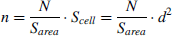
n = \frac{N}{S_{a r e a}} \cdot S_{c e l l} = \frac{N}{S_{a r e a}} \cdot d^{2}

In order to make only one node belong to a cell on average, n should equal to 1, and Eq.(1) can be got Υ

In VGSR, each node determines d according to Theorem 1, which is only a function of S_area and N that can be obtained before deployment. In another words, once sensor nodes know the S_area and N, they can conceive an identical virtual grid in the localization coordinates and make each virtual cell include one node in theory. Figure 2 illustrates the result of construction of virtual cells. From the point of sensor nodes, d could also be the average distance between adjacent nodes.

Figure 2.

Virtual grid and virtual cells.

In the example of Fig. 3.1, N = 400, S_area = 40000 m², according to Eq.(1) the proper d = 10 m. Most cells include only one node and meet the demand of VGSR, but a small part of cells have more than one node and that will lead to address collisions. In order to show the influence of unsuitable d, the result of d = 20 m in the same scenario is given in Fig. 3.2. About 4 nodes in each cell are unacceptable for VGSR. All the results are averaged over 500 simulation runs.

Figure 3.1.

Average number of nodes (d = 10m).

Figure 3.2.

Average number of nodes (d = 20m).

3.2. Address Assignment

As sensor nodes will choose the cell address it belongs to as its address, the assignment of the address for sensor nodes actually equals to the address assignment for the virtual cells. To reduce the address size, there are two basic principles for address assignment:

Limiting address. Because of the fixed address size of VGSR, the size of the address is decided by the maximum value of the cell address. In order to reduce the number of address bits, the maximum address should be limited and address reusing in space is necessary.

Assignment without collision. In communication range of sensor nodes, perhaps, exists several cells. Thus Condition 1 and 2 must be obeyed to guarantee the uniqueness of address in local area.

Before discussion, we give some definitions as follows:

Reusing cell: the cells using a same address;

Reusing distance d_r: the distance between the centers of two adjacent reusing cells;

Address block: a minimum square consists of all cells using different addresses in a local area;

Address size b: the number of bits used to represent address;

Address space Ω: Ω = 2^b;

Needed address A_need: the number of addresses allocated to all cells in the same block;

Spare address A_spare: the number of addresses unused by cells in address space, and it will be used for address collision resolving. A_spare = Ω - A_need.

First, we consider a simple case that a sensor node with communication range R lies in the center of a virtual cell. Thus the distance between two-hop nodes could be 2R at worst. According to Condition 2, the cells in the range of 2R must have distinct addresses. Otherwise, address collision will happen. Figure 4 takes R = d for example. The barred cells must have addresses different from A. In Fig. 4.1, to reduce the number of addresses, the nearest four cells (in gray) beyond the two-hop range are selected as reusing cells. Therefore, the reusing distance d_r is equal to 3d. The other cells among the “A” cells must have distinct addresses, which can also be reused in the same way. All these cells and the A cell in the dark frame constitute an address block together. Despite the worst situation that a sensor node lies in the corner of the center cell, Fig. 4.2 shows that the reusing approach can also work well and that no collision of cell address exists.

Generally, for any R, the reusing distance can be:

d_{r} = (I n t (2 \frac{R}{d}) + 1) d

(2)

where, Int(x) is the smallest integer greater than or equal to x. In a block, all cells need (d_r/d)² addresses. Using Eq.(1), we have:

A_{n e e d} = {(\frac{d_{r}}{d})}^{2} = {(I n t (2 \cdot \sqrt{\frac{λ}{π}}) + 1)}^{2}

(3)

where,

λ = \frac{N}{S_{f i e l d}} \cdot π \cdot R^{2} = ρ \cdot π \cdot R^{2}

(4)

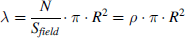
λ is the average connectivity of each node. Therefore, the address size b is:

b = I n t ({log}_{2} A_{n e e d})

(5)

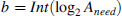
and the number of spare addresses can be expressed as:

A_{s p a r e} = 2^{b} - A_{n e e d}

(6)

Spare addresses are the remaining addresses in the address space, which prepare to resolve address collision (discussed in Section 3.4). According to (6), when log₂ A_need is the integer, all addresses in the address space are allocated to virtual cells, and the spare address is zero. In this case, one more bit is needed by VGSR to set aside spare addresses. Then, the size of the address in VGSR is:

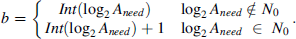
b = {\begin{cases} I n t ({log}_{2} A_{n e e d}) & {log}_{2} A_{n e e d} \notin N_{0} \\ I n t ({log}_{2} A_{n e e d}) + 1 & {log}_{2} A_{n e e d} \in N_{0} \end{cases} .

(7)

Where, N₀ is the set of natural numbers.

Figure 4.

Address spatial reuse.

Based on the discussion above, we get one of assignment pattern for R = d demonstrated in Fig. 5. Nine addresses from 0 to 8 are allocated to virtual cells in a block and only 4 bits is needed correspondingly. The block of addresses is tiled around and the infinite area can be filled in this fashion.

Figure 5.

Address assignment for cells.

Table 1 shows the parameter values for different R, where k = 3,4, … . We do not consider R > d, which means that the communication range is shorter than the average distance between neighbors. The low connectivity in this case will partition the network.

Table 1

Address Assignment for Different R

R	d _r	A _need	b	A _spare
R = d	3d	9	4	7
d < R ⩽ 1.5d	4d	16	5	16
(k − 1)d/2 < R ⩽ kd/2	(k + 1)d	(k + 1)²	Eq.(7)	Eq.(6)

From Eq.(3), the number of addresses is only a function of the average connectivity λ. According to Eq.(3)∼(5), the lower the λ is, the smaller the b is. As the density ρ of nodes is determined by the design of network, we can adjust R to reach the minimum value of b. We summarize the conclusion as Theorem 2.

Theorem 2. The size of the addresses achieves minimum when R = d.

3.3. Mapping

By means of many existing elegant localization algorithms [7], every node could obtain its coordinates (x, y) exactly. As the address in an address block increases from the low-left corner to the upper-right corner regularly, we can establish the mapping as Eq.(8)∼(9).

{\begin{cases} x_{1} = [int (x / d)] mod a \\ y_{1} = [int (y / d)] mod a \end{cases}

(8)

A_{a d d r} = {\begin{cases} 2 x_{1} + y_{1}^{2} & x_{1} \leq y_{1} \\ x_{1}^{2} + 2 y_{1} + 1 x_{1} & > y_{1} \end{cases}

(9)

where, a = d_r/d and int(x) is the largest integer lower than or equal to x. According to Eq.(9), any node can calculate the address A_addr from its coordinates. This simple process is very meaningful for energy-saving.

3.4. Collision Resolving

In VGSR, most cells include only one node, but we cannot exclude the possibility that two or more nodes correspond to a cell in common. In order to enhance the robustness, VGSR takes the scheme which demands address declaration before using to resolve address collision efficiently. When a node detects the address it will use has been declared by the other node preemptively, it usually selects a new one randomly in the spare addresses and declares afresh. Besides, if a node receives a declaration for a spare address, it should inform its neighbors that “the address has been used” to avoid the address collision in the two-hop range of the declarer. Nevertheless, for the extreme case that no spare address is available, the node should turn to sleep. This measure makes sense as too many nodes have clustered in a local area excessively when this happens and it is unnecessary to activate any more nodes so as to save energy. When some nodes are exhausted, the sleeping one substitutes it and uses its address. In order to reduce the overhead, VGSR takes the data packet including the address as declaration in the form of piggybacking.

4. Simulation and Analysis

In this section, we simulate a scenario with N nodes distributing uniformly over a square field with size L × L. Every node sends its first data packet at a random time in an interval of 10 seconds. The results are averaged over 500 simulation runs.

4.1. Typical Scenario

In a typical scenario, N = 400, L = 200m and R = 17.84m, such that λ = 10. Every node is pinpointed. In VGSR, the size of the address is only 5 bits, which can provide 32 addresses. Figure 6 illustrates the using frequency of each address. Based on the curve, most nodes use the address of the virtual cell and the minority obtains the address by collision resolving. The corresponding average size is only 3.86 bits. Compared with the fixed size 5 bits and the average size 4.41 bits of encoded MAC address in [4], when λ = 10 and 9 bits in globe unique address, the performance of VGRS improves greatly.

Figure 6.

The using frequency.

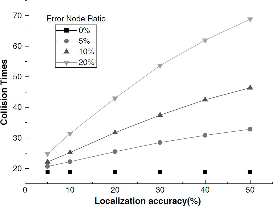
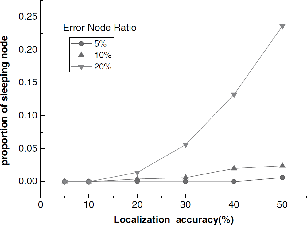
4.1.1 The Influence of Localization Error

Figure 7 shows the relationship between address collision times and localization accuracy [8] when the percent of nodes with localization error denoted by R_Enode is 0%, 5%, 10%, and 20% respectively. The decrease of localization accuracy leads to the increase of collision times directly, which will introduce more extra costs used for collision resolving into VGSR. Figure 8 shows the proportion of sleeping nodes for different R_Enode. Apparently, the inaccuracy of the location information of nodes caused by localization error will impact on the efficiency of MAC address assignment. The more inaccurate the location information is, the more asleep the nodes are. As a result, a part of the nodes can not get effective addresses and are forced to be sleeping falsely, which practically decreases the number of activated nodes in a network. Nevertheless, the curves also show that the VGSR algorithm has fault-tolerant ability to a certain degree. So long as the localization accuracy is comparatively high, VGSR is able to assign an effective address for most nodes.

Figure 7.

The influence of localization error.

Figure 8.

The sleeping node proportion.

4.1.2 Energy Cost

Considering the localization, the energy cost of VGSR is composed of three parts: localization cost, mapping cost, and collision resolving cost, expressed as follows:

\begin{aligned} E_{C} & = E_{L o c a t i o n C} + E_{M a p p i n g C} + E_{C o l l i s i o n C} \\ = f (N) + E_{o p e r a t i o n_1} \cdot T_{M} + E_{o p e r a t i o n_2} \cdot T_{C} \end{aligned}

(10)

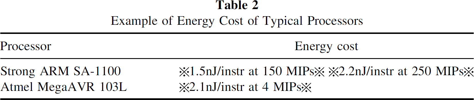
As the location is significant for sensor networks [4], this part of cost represented by f (N), which is often the function of the number of nodes [9], is necessary for any sensor network. The remaining two parts are the actual costs of each node in VGSR. They are determined by the times of mapping T_M and the times of collision resolving T_C respectively. E_{operation_x} is the cost of instruction for corresponding operation. As the overhead of instruction is very low [3] (see Table 2), the energy cost is fairly limited.

Table 2

Example of Energy Cost of Typical Processors

Processor	Energy cost
Strong ARM SA-1100	1.5nJ/instr at 150 MIPs2.2nJ/instr at 250 MIPs
Atmel MegaAVR 103L	2.1nJ/instr at 4 MIPs

4.1.3 Energy Saving

Compared with 9 bits needed by the global unique MAC address for 400 nodes, the energy saved E_s by VGSR is equal to Eq.(11). T_p is the total number of data packets sent by a node, E_bit is the energy for transmitting a bit and the factor 2 represents the address of the sender and the receiver in a packet.

E_{s} = 2 \cdot (9 - 5) \cdot T_{p} \cdot E_{b i t}

(11)

4.2 Overheads

Figure 9 illustrates the overheads of different address assignment schemes. Compared with the encoded MAC address, the overheads of the VGSR algorithm is relatively low. Especially in the case of large connectivity, the improvement of algorithm performance in overheads is remarkable. Although the global unique address has minimal overheads due to the address assignment in advance, no benefit of reducing the address size can be obtained.

Figure 9.

The Comparison of overheads.

4.3 Influence of the Average Connectivity

Figure 10 compares the address size in case of different λ, which varies by changing R of sensor nodes. Obviously, the address size of VGSR is always smaller than that of globe unique. Especially, when R is 10m, namely R = d, the VGSR reaches the minimum size, marked with a circle in Fig. 10. It is the very point that meets Theorem 2. Moreover, the address sizes of VGSR and the encoded MAC address are equal, which means both of them have the same performance in terms of address size.

Figure 10.

The Comparison of address size.

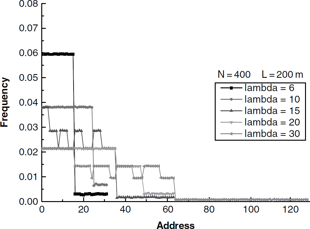
Figure 11 shows the assigning frequency of addresses with different values of λ. In less connected networks (smaller λ), the addresses for virtual cell are reused more frequently. The fluctuation of some curves is because of the edge effect of coverage of virtual cell.

Figure 11.

The using frequency for different λ.

4.4. Scaling Performance

Figure 12 shows how the address of VGSR very with N. Compared with the global unique address, it scales perfectly with the network size. Even at large scale, the address size remains a small value.

Figure 12.

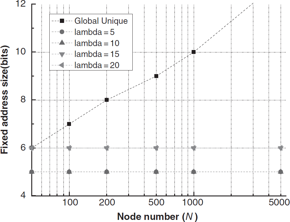
The scaling behavior of VGSR algorithm.

5. Conclusion

In this paper, we have proposed an algorithm to assign MAC address with small fixed size for sensor networks by virtual grid spatial reusing (VGSR), the target of which is to reduce the transmitting energy overhead of networks. Owing to both the address mapping and the piggybacking declaration, VGSR itself is energy-efficient. Our algorithm scales vary well with the size of the network. When the communication range of the sensor node is adjused to the average distance of neighbors, VGSR reach the optimum.

References

Lin

C-Y

Peng

W-C

and Tseng

Y-C

. Efficient In-Network Moving Object Tracking in Wireless Sensor Networks. IEEE Transactions on Mobile Computing, v 5, n 8, August, 2006, pp. 1044–1056.

Elson

Estrin

. Random, Ephemeral Transaction Identifiers in Dynamic Sensor Networks. ICDCS'01, Phoenix, AZ, 2001.

Schurgers

Kulkarni

Srivastava

M. B.

. Distributed On-Demand Address Assignment in Wireless Sensor Networks. IEEE Transactions on Parallel and Distributed Systems, Vol. 13, No. 10, October 2002.

Schurgers

Kulkarni

Srivastava

M. B.

. Distributed Assignment of Encoded MAC Addresses in Sensor Networks. MobiHoc'01, October 4–5, 2001, Long Beach, CA.

Ali

Uzmi

Z. A.

. An Energy-Efficient Node Address Naming Scheme for Wireless Sensor Networks. Networking and Communication, 2004. INCC 204. International Conference on 11–13 June 2004, pp. 25–30.

Dunkels

Voigt

Bergman

and Jönsson

. The Design and Implementation of an IP-based Sensor Network for Intrusion Monitoring. In Swedish National Computer Networking Workshop, Karlstad, Sweden, November 2004.

Loukas

and Radha

. HiRLoc: High-resolution robust localization for wireless sensor networks. IEEE Journal on Selected Areas in Communications, Vol. 24, no. 2, February, 2006, pp. 233–246.

Wang

F. B.

Shi

Ren

F. Y.

. Self-Localization systems and algorithms for wireless sensor networks. Journal of Software, 2005, Vol. 16, no. 5. 857–868. DOI: 10.1360/jos160857

Iyengar

Sikdar

. Scalable and distributed GPS free positioning for sensor networks. Communications, 2003. ICC '03. IEEE International Conference on Vol. 1, 11–15 May 2003, pp. 338–342.