Sage Journals: Discover world-class research

Abstract

In very large-scale dense sensor network applications, more sensor nodes may be deployed than are required to provide the initial desired spatial resolution. Such over-deployment can extend network life, improve robustness, and accommodate network dynamic. To enable large deployments, tiered and clustered network structures may be adopted for scalability and manageability. This article presents a highly scalable, distributed control method to manage the activity of sensors in each cluster so that dynamic application-specific spatial resolution requirement can be achieved with minimum energy cost and with uniform participation of sensors. The method, Look-Ahead Resolution Control (LARC), utilizes a look-ahead prediction of activities of sensors in the cluster and provides feedback to nodes as part of acknowledgments to transmissions. LARC is shown to be highly responsive to system dynamics such as changes in the resolution requested, node failures or replenishment. Existing control methods not only fall short in network life and scalability, but also do not provide such responsiveness and uniform participation to ensure a diverse representation of sensed data. LARC is extended to tradeoff between energy and delay in recovery from failures of large number of nodes, by multiplexing sleeping, listening, and transmissions probabilistically in such a way that the control overhead is minimized while the delay is bounded. The article presents the control strategy for LARC along with performance studies showing near-uniform participation and near-optimal cluster lifetime.

Keywords

Large-Scale Sensor Networks Spatial Sensing Resolution Distributed Control

1. Introduction

Broadly distributed wireless sensor networks (WSN) promise to provide scientific data with very high spatial and temporal resolutions. Large-scale dense sensing applications have emerged from environmental [1], geophysical [2], civil structural [3], ecological [4] sciences and many other research areas. For these and other applications, deployments are envisioned which may utilize tens or hundreds of thousands of sensor nodes. Many believe that large-scale sensor systems are the future trend and therefore a challenge to the sensor network research community [5 8].

Much work to date has been focused on adapting existing computer or wireless networking approaches to the energy constrained realm in which WSN must operate. However, many of these architectures require all nodes to be able to perform routing, processing, etc., all of which increase node cost. For large-scale dense sensing applications, the complexity and cost of such a flat sensor network will become prohibitive. Prior empirical studies [9] found that even simple protocol can exhibit a serious problem of complexity in large-scale sensor network. Tiered and clustered sensor network architectures, e.g., Tenet [8] and two-tier architecture proposed in [10], are promising approaches for large-scale sensor network.

However, as systems become very large in scale, small wastes of energy in every cluster can amount to a large energy squander in the system as a whole. Thus, it is very important to reduce the communications activity within the cluster to a minimum needed to achieve application specific goals. Along these lines, the control communications overhead should also be minimal. In large networks, the number of available sensors is expected to vary as sensors can fail individually due to battery depletion or en masse due to an environmental event. To compensate, new sensors may be added to replenish an existing network. As such, the control method should be adaptive and responsive to both the changes in application-specific resolution requirement and the networks dynamics. Furthermore, to ensure uniform spatial resolution, the participation among nodes should be equal which we also show will achieve maximum network lifetimes.

In this paper, we propose a distributed control method for spatial sensing resolution control within a single-hop cluster in a tiered sensor network. The contributions of this work are as follows:

First, a distributed control method LARC (Look-Ahead Resolution Control) is proposed for controlling the spatial sensing resolution of individual clusters based on the look-ahead prediction of activities of sensors in the cluster from their previous behavior. In this control scheme, sensor nodes are put to sleep when they are not transmitting; and sensors are required to listen to control messages only in the cycles when they are transmitting. The scheme maximizes the cluster lifetime, as it achieves a zero cost in control overhead, excluding energy used in acknowledgements.

Second, to allow applications to tradeoff between energy and delay, or latency, in recovery from failures of large number of nodes, we propose to deliberately add a minimum number of listening cycles and multiplex these listening cycles with transmission cycles in order to achieve a delay that is no larger than the maximum delay tolerance limit specified by applications. We call the LARC method with energy-delay tradeoff LARC-LX, i.e., LARC with listening.

Results from our extensive performance studies show that the proposed control schemes, LARC and LARC-LX, outperform existing methods in terms of both network lifetime and responsiveness, and are highly equal in terms of participation of sensor nodes in the same cluster. That is, LARC closely approaches the ideal performance benchmark, which will be discussed in Section 3, without explicitly knowing the total number of sensors alive. This is a key characteristic since the available sensor population is expected to vary over time as sensors die off or are replenished. In addition, LARC-LX is efficient in allowing applications to trade off between energy and delay in recovery from large failures.

The rest of the article is organized as follows. Related work is discussed in Section 2. In Section 3, we describe the system architecture for large-scale dense sensing, and introduce the spatial sensing resolution control problem. We design and analyze the LARC control protocol and algorithms in Section 4. LARC-LX for energy-delay tradeoff is presented in Section 5. Results from our performance study are presented and discussed at the end of Sections 4 and 5, respectively. Finally, we conclude the work in Section 6, and point out some directions for future work.

2. Related Work

Tiered or hierarchical clustered architectures, such as Tenet [8] and two-tier architecture [10], have been proposed to address the scalability issue in wireless sensor networks. Much work has been devoted to address various issues in such architectures. For example, hierarchical clustering algorithms, such as LEACH [11] and HEED [12], and hierarchical data routing schemes, such as TEEN [13], have been proposed. However, relatively little work has been done on continuous controlling of the spatial resolution of sensor network clusters.

Use of an automaton structure as a basis for a spatial resolution control strategy was first proposed in [14]. This work also first proposed the number of sensors that should be sending information in a wireless sensor network as a measure of QoS for sensor network resolution. That is, the metric governs how much data is coming from the network. Employing a simple Gur game feedback strategy, QoS was shown to be controllable without knowledge of the total number of live sensors, but requiring all sensors to listen for control information continuously. This constraint was removed by using a revised automaton in [15], such that only transmitting sensors were required to listen for control information. The latter automaton, also called the ACK feedback scheme, has been further analyzed in [16] with the following results:

The mean and variance of the achieved QoS can be controlled by selection of automaton parameters;

The method is scalable as the network size increases.

The technique is also expedient in comparison to an equal participating (Bernoulli benchmark) method but there is a tradeoff between variance and network diversity.

However, we found out through simulation (see Sections 4 and 5) that, although the ACK feedback method made a large improvement in responsiveness compared to the Gur game automaton, its response is still relatively slow. What is more, the way probability values are assigned to automaton states is very ad hoc and poor in adaptability. There is no analytical result or theory that determines the probability value assignments, although there are some empirical studies and analyses on various assignment combinations in [16].

The shortcomings of both existing automaton structures, namely the Gur game and ACK feedback control, are:

the participation among nodes in the cluster is not uniform; as such, the work to date has not been able to achieve lifetimes comparable to an equal participating, Bernoulli benchmark; and it is very likely that data from much of the same set of sensors are drawn, leading to undesired biased spatial resolution;

their responses to system dynamics, such as node failures and changes in application requirements, are slow, as we will see in the performance studies.

The key contributions of the work presented herein are to address the first shortcoming while at the same time not requiring knowledge of the total number of sensors alive and not requiring all sensors to listen continuously for control information; and to improve responsiveness by allowing energy-delay tradeoff. Some preliminary findings from our study on the problem of controlling QoS in network resolution appeared in [17].

Recently, growing attention has been devoted to the coverage problem [18, 19]. When coverage is used as a measure of quality of service, the goal usually is to maintain a minimum set of sensors while guaranteeing a certain degree of coverage. A Balanced-energy Scheduling scheme was proposed in [20], to extend the network lifetime of a clustered sensor network while maintaining adequate sensing coverage. However, unlike the coverage problem, in which coverage or sensing ability is assumed to be directly dependent on distance, the spatial sensing resolution problem discussed in this work is only concerned with the number of data points, which is analogous to the number of pixels in a picture, taken as a sample from the area of interest. Although we recognize that coverage can be a useful measure for QoS of sensor networks in applications where sensors are used to detect occurrence of events within their coverage, coverage is not enough for applications that need more detailed numerical characteristics of the field under coverage. What is more, most readings, e.g., light, temperature, and vibration, etc., of a sensor are highly associated with its geographical point of deployment (PoD) in such numerically oriented applications. Characteristics of neighboring locations of a sensor, although spatially correlated with that of its PoD, are not measured accurately by itself. This is our motivation to provide a control mechanism that allows applications to adjust the spatial sensing resolution based on correlation in the physical environment or the needs of the applications. For example, an application may lower the resolution to save energy when it discovers high correlation or similarity among data points, or when it can still guarantee the required accuracy in query results even with lower resolutions in parts of the field. Precision or confidence based probabilistic query processing [21, 22] is a possible application where spatial resolution control may be applied. However, the resolution control problem was not discussed in these works.

3. System Architecture and Spatial Sensing Resolution Control

There are many considerations for a large-scale sensor system. To name a few of the most important ones—robustness, lifetime, scalability, and easiness of management, etc.

A traditional flat wireless sensor network is unlikely to be good candidate architecture for such a system, because it does not have the scalability required. In this paper, we assume a Tenet-like tiered sensor network [8] of single-hop clusters, as illustrated in Fig. 1. Under this architecture, any node in a cluster can only communicate with its clusterhead (CH), which is called master in Tenet, through single-hop wireless connection. That is, each cluster in the network is a single-hop sensor network consisting of a CH and many regular sensor nodes called terminal nodes (TN). Terminal nodes are simple sensor nodes with limited computation and RF capability, while clusterheads are more powerful nodes with better computation and RF capability, equipped with large storage and ample battery energy. Such computation ability enables In-Network processing among clusterheads, where the sensed data is stored. A cluster can be viewed as a virtual sensor node with multiple TNs as sensor boards which are spatially distributed over the space monitored by the cluster, but attached to the CH via a single-hop wireless connection. The readings of sensor nodes within the cluster combined can be taken as the reading of the virtual sensor, whose resolution is controlled by managing the number of active sensors in the cluster. Such architecture extends the sensing scale and increases the sensing density without complicating the network structure.

Figure 1.

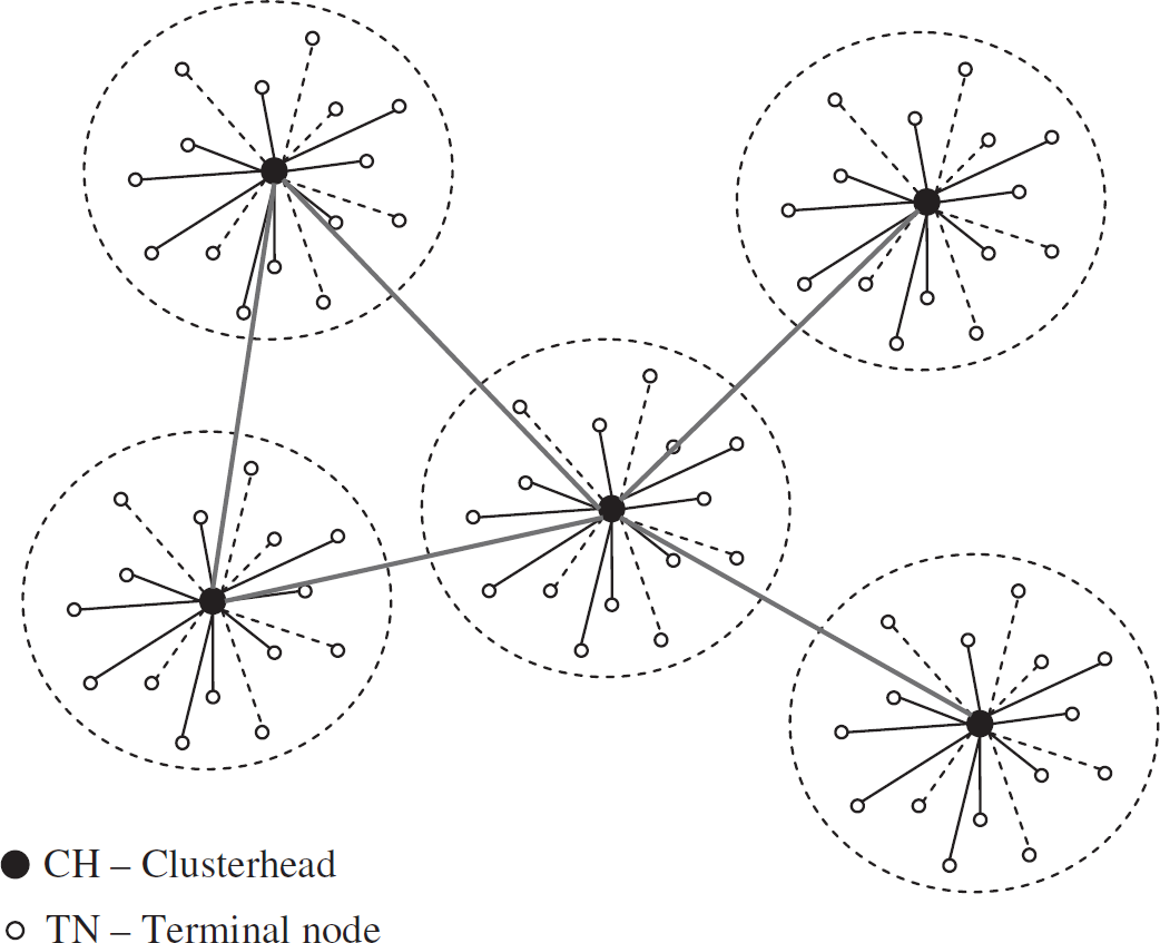
Tiered clustered sensor network system architecture.

Throughout this article, we assume that the temporal dimension is divided into equi-length intervals, each of which is call a cycle (or epoch). Herein, we give the definition of Spatial Sensing Resolution (SSR) as follows.

Definition 1 Spatial Sensing Resolution

For a cluster overdeployed with sensors, the spatial sensing resolution is defined to be K if data are collected from K unique sensors during a cycle.

In other words, spatial sensing resolution is defined as the number of active sensors in a cluster. As the set of data points collected is randomly drawn from all sensors in the area, these data points are expected to be distributed uniformly throughout the area of interest, where a cluster of sensors is deployed. In large and dense deployment, randomness helps

improve equal participation and load-balancing in terms of energy cost, and maximize the network life;

improve the data reliability: in case there is error in readings from some of the sensors random sampling can help avoid getting the same set of erroneous readings repeatedly.

From the view of the sensor network as a whole, unnecessary high resolution in the data gathered by the clusters will incur waste of energy in In-Network processing or routing the data themselves through the network, especially in a large-scale network. Thus we need to control the SSR of clusters to minimum levels (varying from cluster to cluster, and determined by applications) required to achieve application-specific goals. To control the resolution K, i.e., the number of active sensors, to be exactly the desired resolution R is a very difficult problem and the coordination is costly. Therefore, we relax the strict requirement with the following definition.

Definition 2 Statistical SSR

Statistical SSR of a cycle is the expected value of SSR during its time span.

As we will see in the later discussion, statistical SSR can be more practically achieved in a distributed system through collective independent random behavior of participating sensors, with less control overhead. Now, we give the definition of Spatial Sensing Resolution Control as follows.

Definition 3 SSR Control

SSR control is to manage the activity of sensors in a cluster so as to maintain a statistical SSR at the required level R, which is given by the application as a parameter and can be changed over time.

Our design goals for SSR control are

to be energy efficient, minimizing control overhead, thus the network life of a cluster is maximized, and

to be responsive to system dynamics.

Now, let us first take a look at the factors that affect the network lifetime, denoted as LT, of a cluster. Based on energy conservation law, we have the following relation:

E_{T o t a l} = L T \cdot (E [S S R] \cdot r_{TX} + E_{C}) + E_{R}

(1)

Where E_Total is the total sum of energy of all terminal nodes (TN) in the cluster; r_TX is the energy drawn factor for data transmission from a TN to its CH, i.e., energy cost per transmission including ACK; E_C is the control overhead per cycle, which includes costs other than those spent in transmitting reading data, such as costs of listening for control message and response to probing from the CH; and E_R is the residual energy at the end of network life, when provisioning of SSR can no longer be guaranteed. The following equation for lifetime LT can be derived from Eq. (1).

L T = \frac{E_{T o t a l} - E_{R}}{E [S S R] \cdot r_{TX} + E_{C})}

(2)

From Eq. (2), we can see that the lifetime will be increased if the control overhead E_C is reduced or the residual energy E_R is reduced. To design a distributed control method for SSR that minimizes both control overhead and residual energy, with desirable responsiveness, is a big challenge. To see the reason why this is a challenge, let us examine a straightforward attempt to solve the problem.

Suppose the application-required SSR for a cluster under consideration is R; and let N denote the number of sensor nodes (TN) in the cluster that are still alive. Note that both R and N can be varying over time. Every cycle, the CH broadcasts a control message with value p = R/N to all sensor nodes in the cluster; and all sensors nodes need to stay ON in order to keep updated about the control information. In every cycle, each TN decides whether or not to transmit its current reading data to the CH with a probability p, which was received from the CH through the control information. Thus, the statistical SSR is controlled to be exactly N·p = N·R/N = R;

Pros: immediate response to changes in R or N; perfectly equal participation;

Cons: impractically high control overhead in counting N, the number of sensors alive, and requiring the sensor to listen continuously; N must be known to calculate p;

Explicit knowledge of N is requisite to implementation of this control method. However, unless the network (cluster) is continuously queried, N may be unknown. Counting the number of available (alive) sensors costs comparable amount of energy as gathering N reading data. That is to say, the control method at least doubles the energy cost, rather than saving the energy. Nevertheless, its performance in responsiveness and equal/uniform participation is the best that can be achieved, and the statistical SSR is controlled at exactly the required level R. Uniform participation will minimize E_R, i.e., the residual energy. If we exclude the high control overhead in counting N and listening of sensors, i.e., assume E_C to be zero, this control method would also give the optimal performance in terms of lifetime according to Eq. (2). Based on this control method, we defined the following performance benchmark, whose performance is optimal in terms of responsiveness, equal participation, and lifetime.

Definition 4 Bernoulli Performance Benchmark

Assuming that, in every cycle, each sensor node uses a Bernoulli trial with probability of p = R/N to decide if it should transmit its reading data to the CH, where R is the requested resolution and N is the total number of alive sensors in the cluster, and that only transmitting reading data costs energy, the performance thus achieved in terms of responsiveness, lifetime and participation equality is called the Bernoulli Performance Benchmark.

Note that the straightforward method discussed above does not have a performance as the Bernoulli Performance Benchmark (BPB) because energy cost in continuous listening cannot be excluded in real implementation. The control method LARC proposed in this paper address the challenge to approach the performance benchmark in terms of responsiveness, lifetime, and participation equality. In LARC, sensor nodes are not required to listen continuously, as they are in the straightforward method discussed above. Also, LARC totally avoids the overhead in counting N by deriving the control value p from look-ahead prediction based on the previous activities of the sensor nodes. In addition, LARC allows applications to tradeoff energy for responsiveness.

4. Spatial Resolution Control Based on Look-Ahead Prediction

In this section we present the control method LARC, which is the base for LARC-LX to be discussed later in the next section. The goal of the basic LARC is to approach the Bernoulli Performance Benchmark in terms of both lifetime and participation equality.

In our proposed control method LARC, individual sensors will locally make the decision on when (which cycle or epoch) to transmit its next data packet based on a control value, p, provided by the CH as part of an acknowledgement (ACK) for data received. The proposed strategy provides the same control value, p, to and only to the nodes active in the present cycle. As to be detailed in following subsections, the CH determines the appropriate p from look-ahead prediction based on previous activities of sensor nodes in the cluster. Individual sensors then utilize the control parameter to locally determine a schedule for transmitting their next data packet.

Throughout we will assume that the amount of data to be sent in the network is very low in comparison to the available bandwidth; i.e., the network is not bandwidth constrained. This condition can always be achieved by enlarging the cycle length to lower the bandwidth utilization. As such, sensors may employ simple contention based MAC protocols (e.g., ALOHA, slotted-ALOHA or CSMA) with high likelihood that their data packet will get through in the same cycle during which they are sent.

4.1. The Distributed Control Protocol for LARC

We design the control protocol for exchange of reading data and control information between a TN and the CH for the cluster which it belongs to. This protocol is also designed to enable the computation of an appropriate control value p to be sent back to transmitting sensors such that the desired level of sensors activity, i.e., spatial resolution, is maintained.

In this control protocol, every sensor(TN) in the cluster manages its own activity based on the control value p it receives from the CH, such that it has a probability p of transmitting (TX). If a TN is not transmitting during a cycle, it may turn off the radio and go into a sleep mode to save energy. Nevertheless, it maintains a transmitting probability of p in every cycle. On the other hand, the CH collects and stores the data packets it receives from the TNs under its cluster. Note that the number of data packets is defined as SSR. The CH also does some book-keeping of the sensor activities based on these data packets received. At the beginning of a cycle, the CH computes a control value p based on the SSR required by application and the previous activities of sensors. Each time the CH receives a data packet from a TN, the CH will send back an ACK packed with the control value p for that cycle. Figure 2 shows a diagram illustrating the protocol.

Figure 2.

Diagram of the distributed control protocol.

The advantage of this protocol is that every sensor node manages its own activity autonomously only based on the last control information, i.e., the value p, received from the CH. That is to say, the sensor node only needs to keep a schedule of transmitting and sleeping in such a way that, in each cycle, it has a probability p to be transmitting. Neither does a TN need to know what is the current SSR required by application, nor does it need to know how many of its peer TN are still alive. There is no coordination between any two TNs. In Section 4.2, we will discuss how the individual TNs manage their own activities independently of each other. The management scheme is very energy-efficient since it allows sensors to shut off both radio and processing unit completely when they are not transmitting.

In Fig. 2, the timer value v_t denotes the number of cycles the TN has been sleeping since the transmitting of its last data packet. The CH needs this information for book-keeping the activities of the sensors to facilitate the calculation of look-ahead prediction, from which an appropriate p is derived, as will be discussed later in Section 4.3. Since TNs that show up in the same cycle will receive the same control value p, they can be viewed as a group identified by that cycle. When a TN wakes up to transmit a data packet, it also sends along its timer value v_t along with the packet. Thus, the CH knows when this TN transmitted its last data packet and excludes it from the corresponding group of sensors as the TN now gets a new control value.

As ACK is presumed to be necessary for transmission acknowledgement anyway, the control protocol actually incurs no control overhead (except the negligible increase in packet size), since the exchange of control related information, i.e., p and v_t, are carried through the ACK and data packet respectively. Thus, this distributed control protocol has a zero control overhead in some sense.

4.2. Sensor Node Autonomous Management of its Own Activity

As we pointed out earlier, in LARC each sensor manages its own activity, i.e., transmitting or sleeping, only based on the control value p received from the CH. The sensor only needs to maintain its activity schedule such that, in every cycle, it has a transmitting probability of p. The simplest way is to perform a Bernoulli trial every cycle, with a probability of p, to decide whether it should transmit in that cycle. More specifically, a sensor node generates a random number uniformly from the range [0, 1]. If the number generated is with the range [0, p], it will transmit in that cycle. In this way, it maintains a transmitting probability of p in every cycle. However, the sensor is required to keep the processing unit on in every cycle just for the purpose of the Bernoulli trial. It is a waste of energy to have the processing unit on to perform the test every cycle even when it is unlikely that the sensor is going to transmit.

To avoid such inefficiency in energy, we propose a timer-based scheme for self-management of a sensor's own activity. The key idea is to perform multiple Bernoulli trials in advance to determine when is the next cycle the sensor is going to transmit. Thus, the sensor may be safely put into sleep during cycles in between one transmitting cycle and the next. The timer value v_t denotes the number of cycles the sensor is allowed to sleep before the next sampling and transmission of reading data. Before a sensor goes into sleep it resets its own timer with value v_t. Upon waking up by the timer, a TN will transmit the sampled reading data along with v_t to the CH. The detailed algorithm for sensor self-management is shown in Algorithm 1.

In implementation of the timer-based control, we imposed an upper bound T_UB (each sensor has its own T_UB, which depends on the value p received from the CH) on the timer value v_t to avoid the case of any sensor having too low of a response rate, as in some rare, if not impossible, cases the trial can fail many times and v_t becomes very large. An appropriate T_UB can be derived from the control value p as follows, where the random variable k is the number of failures between two successes of the Bernoulli trials.

P (κ \leq T_{U B}) = \sum_{k = 0}^{T_{U B}} P (κ = k) = \sum_{k = 0}^{T_{U B}} (1 - p)^{k} \cdot p = 1 - (1 - p)^{T_{U B} + 1} \geq 1 - α

(3)

Algorithm 1.

Sensor transmission rate control.

Here, it has a confidence of 1–α that a sensor with transmission probability p will transmit another data packet in no more than T_UB cycles. Thus, in setting this upper bound, we use the minimum T_UB value satisfying (4) derived from $1 - (1 - p)^{T_{U B} + 1} \geq 1 - α$ in (3).

T_{U B} \geq \log (α) / \log (1 - p) - 1

(4)

Where α can be set for desired confidence. For example, α = 0.05 means that the TN has a 95% confidence to transmit its next packet within the next T_UB cycles. Thus, the TN is not allowed to sleep for more than T_UB cycles.

4.3. Determine the Appropriate Control Value p at the CH

Upon receiving a data packet from any of the TNs, the CH will do some book-keeping of control related information. This information will later be used in the look-ahead prediction for the purpose of calculating an appropriate control value p to be sent to transmitting TNs. The control value is recalculated at the beginning of every cycle, and the same control value is sent back to all transmitting TNs during that cycle.

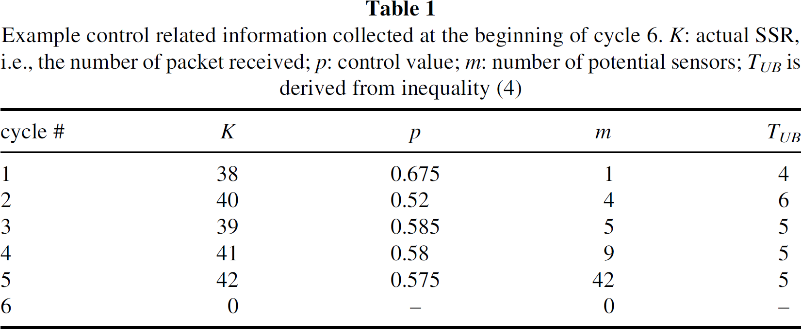
The control-related information collected at the CH is on a cycle-basis, and includes a timestamp of a cycle, number of packets received during that cycle, control value used for that cycle, and the number of potential sensors defined as follows.

Definition 5 Potential Sensors

The potential sensors of a cycle t are those sensors that have transmitted during the cycle t and have not transmitted another data packet yet and are still alive.

Since potential sensors of a cycle have not transmitted another packet yet, their control values are not updated. That is, their control values are still the same as that is associated with that cycle. The CH can simply look up the control-related information it stored to obtain this value associated with that cycle. The number of potential sensors of a cycle can be counted at the CH as follows. When the CH receives a data packet, it knows how long the TN has been sleeping before sending this packet, based on the timer-value v_t enclosed in the packet. Thus, the CH can infer when (which cycle) this TN sent its previous data packet, and reduce the counting of potential sensors for that cycle by one.

Table 1 shows what the control-related information collected at the CH looks like. This example shows a snapshot of control related information collected at the CH at the beginning of cycle 6. The counting variables K and m are initialized to be zero. The control value p for cycle 6 is yet to be calculated, as will be discussed later. After p is determined, T_UB can be derived from inequality (4) by plugging in the value of p.

Table 1
Example control related information collected at the beginning of cycle 6. K: actual SSR, i.e., the number of packet received; p: control value; m: number of potential sensors; T_UB is derived from inequality (4)

cycle# K p m T_UB

1 38 0.675 1 4

2 40 0.52 4 6

3 39 0.585 5 5

4 41 0.58 9 5

5 42 0.575 42 5

6 0 — 0 —

cycle#	K	p	m	T_UB
1	38	0.675	1	4
2	40	0.52	4	6
3	39	0.585	5	5
4	41	0.58	9	5
5	42	0.575	42	5
6	0	—	0	—

Algorithm 2 shows how the CH response to data packet received from a TN, and how control-related information is maintained at the CH.

Now we proceed to show how the appropriate control value p is calculated at the CH using look-ahead prediction based on the control-related information collected. This calculation is performed at the beginning of each cycle, and the same control value p thus calculated is sent back to every TN that transmits during that cycle.

Figure 3 shows the look-ahead prediction model for computing the appropriate control value at the CH given R as the required SSR. For simplicity of discussion, the cycles are indexed backward. Suppose it is now at the beginning of the current cycle e′, and a control value p needs to be calculated for the cycle e′. Any TN that later sends a data packet during cycle e′ will receive an ACK with this control value p.

Algorithm 2.

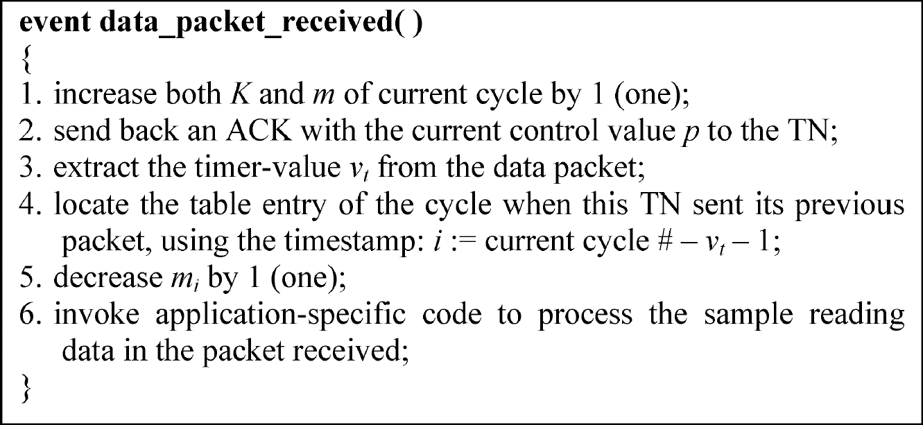
CH response to packet arrival and collecting of control related information.

Figure 3.

Illustration of the look-ahead prediction model.

To determine an appropriate control value to be used in cycle e′, we derive the probability distribution of the SSR, i.e., the number of packets received, of its next cycle e″, assuming the control value of cycle e′ to be p. That is to say, this is a p-parameterized probability distribution for the random variable K, which is the SSR of the cycle e″. By tuning the parameter p, we manage to make K approach R, i.e., the required SSR.

Let K_i denote the number of packets received during cycle i as is indexed in Fig. 3. Similarly, p_i is the control value and m_i is the number of potential sensors respectively for cycle i. Take any of these m_i sensors of cycle i for example, since this sensor has not sent any packet until now (otherwise it should not have been counted in m_i), the probability that it will send a data packet during the cycle e′ is exactly p_i, the control value used in cycle i:

{p^{'}}_{i} = p_{i}

(5)

And, the probability that the sensor will send its next data packet during the cycle e″ is:

{p^{''}}_{i} = (1 - p_{i}) \cdot p_{i}

(6)

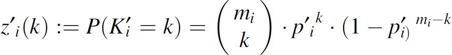
Let random variable K′_i denote the number of these m_i sensors that will send a packet during the cycle e′. Then K′_i follows a binomial distribution, i.e., K′_i ∼ Bi(m_i, p′_i). That is, z′_i(k), the pdf for K′_i is:

{z^{'}}_{i} (k) := P (K_{i}^{'} = k) = (\begin{matrix} m_{i} \\ k \end{matrix}) \cdot {p^{'}}_{i}^{k} \cdot (1 - p_{i}^{'})^{m_{i} - k}

(7)

Likewise the pdf for the random variable K″_i, the number of those m_i sensors that will send their next data packet during the cycle e″, is:

z_{i}^{''} (k) := P (K_{i}^{''} = k) = (\begin{matrix} m_{i} \\ k \end{matrix}) \cdot {p^{''}}_{i}^{k} \cdot (1 - {p^{''}}_{i})^{m_{i} - k}

(8)

Let random variables K′ and K″ be defined for e′ and e″ (see Fig. 3) respectively as:

K^{'} = K_{1}^{'} + K_{2}^{'} + \dots + K_{i}^{'} + \dots + K_{M}^{'}

(9)

and

K^{''} = K_{1}^{'} + K_{2}^{''} + \dots + K_{i}^{''} + \dots + K_{M}^{''}

(10)

where M is the maximum memory size under the consideration. The random variable K′ means the number of sensors that will send a data packet during cycle e′; while K″ means the number of sensors that will send their next data packet during cycle e″, instead of cycle e′. As our mechanism for decrementing the m_i ensures the independency between the random variables at the right-hand side of (9), the pdf of K′ can be determined as the convolution of the individual pdfs of all K′_i; that is,

K^{'} \sim z^{'} = z_{1}^{'} ⨂ z_{2}^{'} ⨂ z_{2}^{'} ⨂ \dots ⨂ z_{M}^{'}

, where ⨂ is the convolution operator. So P(K′ = k) = z′(k). Likewise P(K″ = k) = Z″(k), where the pdf

z^{''} = z_{1}^{''} ⨂ z_{2}^{''} ⨂ \dots ⨂ z_{M}^{''}

Let random variable K_e′ be the number of sensors that will send another data packet during the cycle e″ amongst the K′ sensors that send a data packet during cycle e′ and thus get a control value update p. Then we have

P (K_{e^{'}} = k | K^{'} = u) = {\begin{cases} (\begin{matrix} u \\ k \end{matrix}) \cdot p^{k} \cdot (1 - p)^{u - k} & , 0 \leq k \leq u \\ 0 & , k > u \end{cases}

(11)

Recall that the parameter variable p is the control value to be used during cycle e′. By averaging over all possible K′ values, we can obtain the following approximate distribution of K_e′

\begin{aligned} P (K_{e^{'}} = k) = & \sum_{u = 0}^{\hat{K}} P (K^{'} = u) \cdot P (K_{e^{'}}) = k | K^{'} = u) \\ = & \sum_{u = k}^{\hat{K}} z^{'} (u) \cdot (\binom{u}{k}) \cdot p^{k} \cdot (1 - p)^{u - k} \end{aligned}

(12)

where $\hat{K}$ is the maximum possible K′. Finally, let random variable K be the SSR, i.e., number of packets that will be received, of cycle e″, then it can be seen from Fig. 3 that K = K″ = K_e′. Thus

\begin{aligned} P (K = k) = & \sum_{v = 0}^{k} P (K_{e^{'}} = v) \cdot P (K^{''} = k - v) \\ = & \sum_{v = 0}^{k} P (K_{e^{'}} = v) \cdot z^{''} (k - v) \\ = & \sum_{v = 0}^{k} (\sum_{u = v}^{\hat{K}} z^{'} (u) \cdot (\binom{u}{v}) \cdot p^{v} \cdot (1 - p)^{u - v}) \cdot z^{''} (k - v) \end{aligned}

This gives the probability distribution of SSR of cycle e″, with variable p as a parameter, which is the control value to be used in the cycle e′. Thus, we choose a value of p to maximize the probability that K is close enough to R, the required SSR:

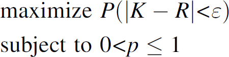
\begin{aligned} maximize P (| K - R | < ε) \\ subject to 0 < p \leq 1 \end{aligned}

Where the probability distribution of K is given by (13), and the error bound ϵ may take a value of 1 or 2 in practice. The optimal value of p thus obtained is used as the control value for the cycle e′. Such calculation of control value p occurs once every cycle at the beginning of that cycle. Any TN that transmits a data packet during that cycle will receive the same control value.

4.4. Dealing with Failure of Sensor Nodes

When there is an abrupt event that causes a large number of sensor nodes to fail, the total number of sensors available in a cluster will drop dramatically after the event, and the control related information m_i collected before at the CH can be larger than the actual number of sensors alive with transmitting probability p_i, if cycle i happened before that event. Under LARC protocol, it is impossible for the CH to know if a sensor node has failed or is still alive. Thus, there need to be some mechanism to correct m_i, the number of cycle i potential sensors, when the CH finds that the number of packets received during a cycle is unlikely to be coming from to the optimal distribution of K given the optimization at the end of Section 4.3, i.e., when node failures are detected by the CH.

In LARC, a Two-Step Maximum Likelihood Estimator is used to estimate the number of potential sensors m_i in case of observing unexpected low network activity, which is due to node failures. This two-step estimator requires additional control-related information r_i,1 and r_i,2 which are the number of packets received from the cycle i potential sensors during the last cycle and the last second cycle. The likelihood function of an estimator ${\tilde{m}}_{i}$ for m_i (at the end of last cycle) is defined as follows.

L ({\tilde{m}}_{i}) = (\begin{matrix} {\tilde{m}}_{i} + r_{i, 1} + r_{i, 2} \\ r_{i, 2} \end{matrix}) p_{i}^{r_{i, 2}} \cdot (1 - p_{i})^{{\tilde{m}}_{i} + r_{i, 1}} \cdot (\begin{matrix} {\tilde{m}}_{i} + r_{i, 1} \\ r_{i, 1} \end{matrix}) p_{i}^{r_{i, 1}} \cdot (1 - p_{i})^{{\tilde{m}}_{i}}

(14)

That is, the probability that r_i,1 and r_i,2 were observed respectively in the last two cycles given the condition that there are ${\tilde{m}}_{i}$ sensors alive with transmitting probability pi after the last cycle. The two-step maximum likelihood estimator is given by:

{\hat{m}}_{i} = \arg max_{{\tilde{m}}_{i}} {L ({\tilde{m}}_{i})}

(15)

In the implementation of LARC, the CH will correct m_i with the estimator ${\hat{m}}_{i}$ if it determines that K₁, the actual number of data packets collected in the last cycle, is very unlikely based on the optimal distribution. That is to say, the correction is made when the CH finds that P_OPT(K ≤ K₁) is less than a correction threshold α, e.g., α = 0.01, where P_OPT(K = k) is the optimal distribution of K for the last cycle as discussed at the end of Section 4.3.

4.5. Performance Studies

In this subsection, we will present and discuss results from performance studies of the proposed LARC distributed control method, and compare it to the existing Gur and ACK feedback control methods, along with the ideal equal participating Bernoulli Performance Benchmark (BPB). As clusters in the network control their resolutions independently of each other, our simulation studies only focus on a single cluster.

Table 2 summarizes the settings used throughout the simulation studies. The CH is assumed to have infinite or orders of magnitude larger energy capacity than other sensor nodes such that it dies only after all sensor nodes have died. A cluster of size 1000 is considered large enough, since a system with tens of clusters will have tens of thousands of nodes.

Table 2
Simulation settings

Setting Meaning Values

N Total number of sensors available in a cluster 5 to 1000

R Statistical SSR requested 5 to 100

C _LX Energy draw per listening (low-power listening) 1

C _TX Energy draw per transmission (from TN to CH) 2

E ₀ Initial energy at each sensor node (TN) 1000

E _CH Initial energy at the clusterhead +∞

ϵ Optimization error bound for maximize $P (| K - R | < ε)$ 1

Setting	Meaning	Values
N	Total number of sensors available in a cluster	5 to 1000
R	Statistical SSR requested	5 to 100
C _LX	Energy draw per listening (low-power listening)	1
C _TX	Energy draw per transmission (from TN to CH)	2
E ₀	Initial energy at each sensor node (TN)	1000
E _CH	Initial energy at the clusterhead	+∞
ϵ	Optimization error bound for maximize $P (\| K - R \| < ε)$	1

In these simulation studies, the Gur control is implemented as described in [14]; and ACK feedback control is implemented with five-state automata, with probability values [0.045 0.76 0.95 0.999 0.99999], which has been shown to be effective in [16].

4.5.1. Correctness of Control

In the first study, we simulated a deployment of a cluster of N = 100 sensors. In these simulations, it is assumed that a sensor will die if and only if it runs out of battery, i.e., no other failure mechanisms. We examined the correctness of the three control methods, namely Gur, ACK feedback and LARC, under various settings.

Figure 4 shows the mean SSR achieved by each control method at different points of time over a period of 1500 cycles, where the SSR requested is R = 40. The mean SSR was measured from 100 runs of the simulation. At the beginning, it took Gur control about 100 cycles on average to converge to the desired R; and at the time 500, around 40 of the sensors die under Gur control due to depletion of energy, as also can be seen in Fig. 5. It took Gur more than 200 cycles to recover from this loss of sensor nodes. It can be seen from Fig. 4 that the cluster lifetime under Gur control is much shorter than other methods. This is because of that Gur requires all sensors to listen continuously, i.e., on every cycle. ACK feedback control performed much better, but its mean SSR is around 39, and is slightly lower than the desired R = 40. LARC maintained a mean SSR that is very close to the BPB and its SSR lasted longer at this level than both Gur and ACK feedback, approaching the ideal BPB.

Figure 4.

Statistical SSR over time (R = 40).

Figure 5.

Number of alive sensor over time (R = 40).

Figure 5 shows the number of sensors alive during the same time period under each control method. The number of sensors alive in both Gur and ACK feedback dropped from the initial 100 very quickly after the first half the whole lifetime of the cluster. On the contrary, LARC maintained the total number of sensors alive to be at the initial level until the very end of the cluster life, just as the ideal BPB did. This benefit is especially important when the application needs to adjust to a higher SSR during the later part of the cluster lifetime. For example, ACK feedback would not have been able to make it should the application change the required R from 40 to 80 starting at the time 1000, since there were only about 70 sensors available/alive in the cluster at that time. It is even worst for Gur control. As will be shown later, this benefit in LARC is a result from the uniform participation it has.

Simulations were done on various R requested and cluster size N to see how each control method works under various settings of R and N. In these simulations, sensors were initialized with enough energy such that none of the sensor died before the simulation ended. Figure 6 shows that the approximate operating region of Gur control is between R = 35 to 70, i.e., 35% to 70% of the cluster size N = 100. Both ACK feedback control and LARC have full operating region from nearly 0% to 100% of cluster size. But the SSR achieved by ACK feedback control is slightly lower than the requested R in most cases. Figure 7 shows the resulting SSR achieved by each control method when the requested R is fixed at 10 and the cluster size varies from 10 to 50. The Gur method has only a limited operating region. The Gur control can easily go out of its operating region as R requested by application changes or cluster size changes due to node dying off or replenishing. The Gur control method always gives half of the cluster size outside of its operating region. Thus the SSR achieved by Gur scales up as the cluster size become larger, instead of locking at the requested level R. Simulation was also done for cluster size N = 50 to 1000. The SSR of Gur scaled up linearly to 500, i.e., half of 1000. The SSR of ACK feedback control also scaled up linearly to nearly 50 when the cluster size became larger, because a sensor has a transmitting probability of at least 0.045 even in the least active state in the ACK feedback automata. LARC is highly scalable. The SSR of LARC always locked at the requested level R = 10 for cluster size N = 10 to 1000 in the simulation.

Figure 6.

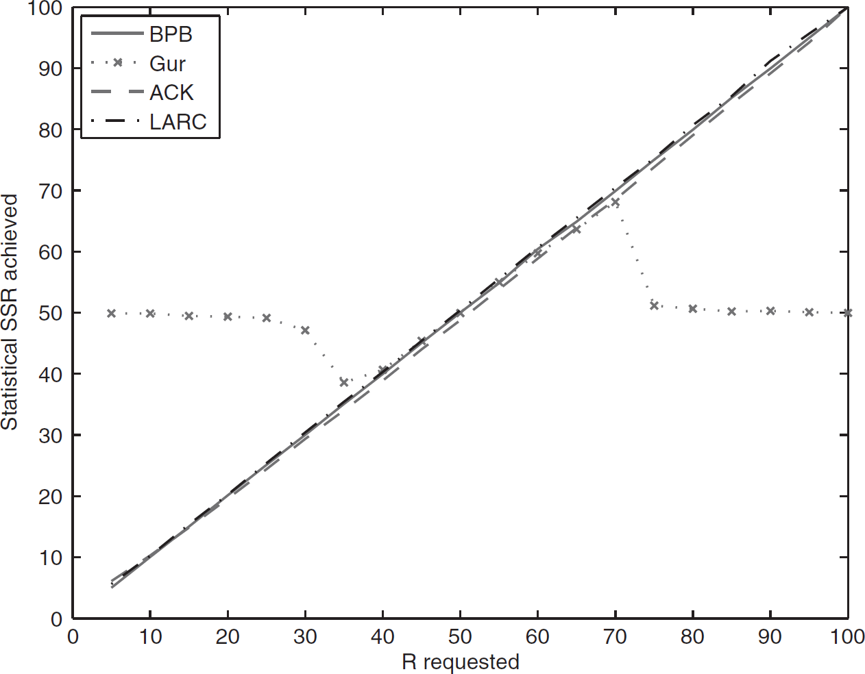
SSR achieved vs requested (N = 100).

Figure 7.

SSR achieved vs total number of sensors available (R = 10).

Uniform participation, which means every sensor node has the same chance of contributing, is one desirable property of resolution control methods from both the data collecting and energy perspectives. Uniform participation also helps maximize individual sensor lifetime and keep the total number of sensors alive higher for a longer period of time than non-uniform participation. Figure 8 shows the histogram of participations of N = 100 sensors over a period of 5000 cycles, where R requested is 40 and each sensor has energy enough for 10000 cycles. In BPB and LARC, sensors mostly have a participation count of around 5000 × 40/100 = 2000 times, and participation counts of sensors range from 1900 to 2100, i.e., ±5% around 2000. In Gur control, participation counts of sensors are polarized. A number of 40 sensors participate almost all the time; while the rest of the 60 sensors have nearly no participation. In ACK feedback control, node participation counts range from 1000 to 3000, i.e., ±50% around 2000. Thus sensors under ACK feedback control do not participate as uniformly as in BPB and LARC.

Figure 8.

Histogram of participation counts.

4.5.2. Cluster Lifetime and Energy Efficiency

In the following simulation study, our concern is the performance of control methods in terms of cluster lifetime and energy efficiency. We used limited energy settings given in Table 2. Let us define Cluster Service Life as following:

Cluster Service Life = max {t|T — cycle moving average of SSR over time t to t + T is no less than R}

Where T = 5 in our simulations. That is, time t is considered to be the end of the cluster service life if 5-cycle moving average of SSR after that point is always below the requested level R.

Figure 9 presents the lifetime performance of each of the control methods. Lifetime becomes shorter as R, the requested SSR, is larger. Again cluster lifetime under LARC approached the ideal BPB closely. Cluster lifetime under ACK feedback control is shorter in comparison to LARC. Cluster lifetime under Gur control is the shortest among all control methods. Figure 10 shows the difference more clearly in terms of percentage of the lifetime under BPB, which is the ideal case. LARC achieved a cluster lifetime of nearly 100% that of BPB for all R requested. The ACK feedback control only achieved around 90% that of BPB on average.

Figure 9.

Cluster service life vs R requested.

Figure 10.

Cluster service life (in % of BPB) vs. R requested.

Figure 11 shows the amount of residual energy at the end of the cluster lifetime under each control method. Because of non-uniform participation in Gur and ACK feedback control, sensor nodes also die off non-uniformly, resulting in a large amount of unused residual energy at the end of the cluster service life. This residual energy is wasted as there are no longer enough sensors to meet the requirement of R requested. Mostly around 20% of total energy was wasted as residual energy at the end of cluster life in Gur or ACK feedback control. Much less (mostly less than 5%) of the total energy was wasted in LARC as compared to Gur and ACK feedback control. As we can see from Eq. (2), minimizing residual energy also helps to improve the lifetime of a cluster.

Figure 11.

Residual energy E_R (in % of initial energy in system) vs R.

4.5.3. Responsiveness

Finally, we simulated uniform random sensor nodes failure to see how quickly each control method recovers from the failure. When there was a drop in N, the total number of sensors available in the cluster, we observed a corresponding drop in the SSR under each control method. We simulated the drop in N at one time point and measured the time it took for each of the control methods to get the SSR back to the requested level.

The result is shown in Fig. 12. In most cases Gur control has a very large delay. ACK feedback control and LARC have similar but much smaller delay in comparison to Gur control. LARC slightly outperforms ACK feedback control when there is a larger failure. However, the delay can be as large as 50 cycles when 95% of the nodes failed and the cluster was operating at R = 10 with initially 200 sensors. We can see that when the failure ratio is high, the delay (in either ACK or LARC) in recovery of SSR can be larger than what the application can tolerate, especially some real-time applications. In Section 5, we will discuss how to improve the responsiveness of LARC by adding extra listening cycles.

Figure 12.

Delay; fixed R = 10; N drops from 200 to N X (1-failure_ratio) at time t = 50.

5. Spatial Resolution Control with Energy-Delay Tradeoff

Although LARC has been shown to have a faster response compared with Gur and ACK, the delay may still not be small enough for some applications that require real-time control over the resolution, especially when the cluster is operating at a low resolution level, as we have seen in Fig. 12. In this section we propose LARC-LX, which deliberately multiplexes some listening (LX) with the transmissions (TX) to improve responsiveness. Listening can cost less energy than transmitting [23]. Technologies like low-power listening on paging channel [24] have made listening even much cheaper than transmitting. However, we still do not want to have all sensors listening and wasting energy unnecessarily. Thus, the problem here is to determine a minimum amount of extra listening, during non-transmitting cycles, such that the desired responsiveness is achieved. This is a tradeoff between the energy cost and delay in response.

The ideal Bernoulli Performance Benchmark assumes all sensors listen to the control message from the clusterhead (CH) in every cycle. The benefit of listening all the time is a fast response when there is any change in the system. The ideal Bernoulli Performance Benchmark takes only 1 cycle to respond: all sensors receive a control message once it is broadcasted; and the control message takes effect immediately from the next cycle on. However, listening (LX) also incurs unnecessary energy consumption, especially when such changes occur only occasionally and the application can tolerate certain delay in the adaptation (R ramps up) or recovery (from large drop in N). On the other extreme, non-listening control methods, namely ACK control and LARC, totally avoid the cost of extra listening by shutting off the radio and putting the sensor to sleep respectively when it is not transmitting (TX). Thus, not all the sensors are reachable when there is a sudden change in the system, and the CH needs more sensors to supply the lost/failed sensor or the rise in demand.

To improve responsiveness energy-efficiently, we propose LARC-LX, which is a tradeoff between always-listening control and non-listening control. In LARC-LX, extra listening cycles are deliberately added and multiplex with TX cycles based on the non-listening LARC such that the delay in response is bounded by the maximum-tolerate-limit (MTL) specified by application.

5.1. Response Delay and Materialization of Controls Information

Now, let us first look at how the delay in response is dependent on the materialization of control information from the CH at individual sensors. In the next subsection, we will show how to determine extra listening based on this relation.

Let CX denote the event that the control information for the current cycle is materialized at a particular sensor node (TN), i.e., this TN receives the control message from the CH either by listening (when not transmitting) or by extracting that from the ACK to its transmission in the current cycle. In other words, CX event at a particular TN means that the TN is updated with current control information. In non-listening control methods, such as ACK feedback control and LARC, CX is equivalent to the event TX because only transmitting sensors get updated with current control information.

Now let us suppose some destructive event happens in the environment where the system is deployed. Assume this destructive event destroys/disrupts a large number of sensor nodes uniformly randomly, thus drops the total number of available sensors in a cluster from N to N′. At the CH side, it will see a sudden drop in SSR as the remaining alive sensors continue to operate in the same way as before until they are updated with current control information, i.e., CX occurs. We assume that the CH will be sending a control message to ask listening and transmitting sensors to stay ON and continue TX for the cycles thereafter to ramp up the SSR. This adaptation process is shown in Fig. 13. We would like to know how long (Δ_τ) it takes for the SSR to go back to the requested level R, given that every alive sensor has a probability P(CX) of being updated with the current control information, which asks the sensor node to stay ON.

Figure 13.

The adaptation process.

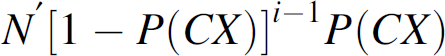
It can be seen that the mean number of survival sensors that will get their first control message from the CH during the i^th cycle since the drop is:

N^{'} [1 - P (C X)]^{i - 1} P (C X)

(16)

According to our assumption, these sensors are requested by the CH to stay on duty in order to ramp up the SSR. Let Δ_τ be the number of cycles it takes for the SSR to go back the requested level R (see Fig. 13), then we have the following relation:

\sum_{i = 1}^{Δ τ} N^{'} [1 - P (C X)]^{i - 1} \cdot P (C X) = R

(17)

That is,

\frac{1 - [1 - P (C X)]^{Δ τ}}{1 - [1 - P (C X)]} P (C X) = \frac{R}{N^{'}}

(18)

Thus, the delay Δ_τ is:

Δ τ = \frac{\log (1 - R / N^{'})}{\log (1 - P (C X))} = \frac{\log (1 - P (T X) / F)}{\log (1 - P (C X))}

(19)

Where the survival ratio F = N′/N R/N, and transmitting probability of survival sensors is P(TX) = R/N. In non-listening controls such as ACK feedback control and LARC, P(CX) = P(TX); while in always-listening control P(CX) = 1, which means Δ_τ = 1 based on (17).

5.2. Multiplexing TX and LX to Improve Response

In non-listening LARC, when the requested R is very low, P(CX), which equals P(TX), may not be large enough to bound the delay as specified by the application. In this section, we show how extra listening (LX) cycles are multiplexed with transmissions (TX) cycles to increase P(CX), such that the delay is bounded as specified by the application.

In addition to the timer used to control TX in LARC (see Section 4.2), another timer is added to the sensors for the purpose of controlling LX. These are two independent timers which are controlled by two independent random number generators respectively. The TX timer is controlled by the control value received from the CH, such that the transmitting probability P(TX) of the sensor is equal to the control value (see Section 4.1). Let P(LX) be the probability of listening controlled by the LX timer. Since a sensor is updated with the current control information from the CH, either when the sensor is listening (LX) or when it is transmitting (TX), we have the following relation:

P (C X) = 1 - P (\bar{T X}) \cdot P (\bar{L X})

(20)

Thus, we have

P (L X) = 1 - P (\bar{L X}) = 1 - \frac{1 - P (C X)}{1 - P (T X)}

(21)

By solving Eqs. (19) and (21) together, with P(CX) and P(LX) as unknown variables, we will get a value for listening probability P(LX). If the LX timer controls the sensor to wake up with a probability of P(LX) to listen to the control message from the CH, we are guaranteed that the delay is bounded by Δ_τ specified by the application, provided that F used in (19) is the worst-case survival ratio.

5.3. Modified Responding Protocol

To utilize extra listening for improving the responsiveness, we modify the original LARC protocol so that listening sensors know how to react when their participation is needed. In this modified control protocol, the CM (control message) from the CH contains a listening probability value and an emergency bit in addition to the transmitting probability value, i.e., control value, in the original LARC protocol. The listening probability value, given by (21), in the CM tells a sensor how often it should be listening. Listening but not transmitting sensors change their transmitting probability to the control value specified in a CM only if the emergency bit in the CM is 1. Thus listening but not transmitting sensors will only change their transmission behavior when their participations are needed.

At the CH, the emergency bit in the control message is set to 1 if the peak of the resulting optimal distribution (given by the optimization following (13)) is on the left side of R − ϵ, which is the optimization lower error bound. That is to say, the emergency bit is set to 1 to bring in extra listening sensors if the cluster will be likely to collect fewer than R − ϵ data packets during next cycle according to the optimal distribution.

5.4. Performance Studies

In the following, results from the simulation studies on LARC-LX are presented. As the Gur control is out of the operating region and slow in response as we have seen in subsection 4.5, we only compared the responsiveness of ACK feedback control and LARC-LX. We simulated the following LARC-LX schemes with fixed lower bound on P(CX):

LARC-LX0: extra listening is added in such a way that P(CX) equals max{0, P(TX)}, i.e., no extra listening is added. This is the same as non-listening LARC;

LARC-LX1: extra listening is added in such a way that P(CX) equals max{0.1, P(TX)}, i.e., extra listening is added so that P(CX) is no less than 0.1;

LARC-LX2: extra listening is added in such a way that P(CX) equals max{0.2, P(TX)}, i.e., extra listening is added so that P(CX) is no less than 0.2;

In all the schemes above, sensor listening probability P(LX) is given by (21) based on the respective P(CX).

First, we simulated a large drop in the total number of sensors available in the cluster, and see how quickly each control method will get the SSR back to the requested level. As shown in Fig. 14, SSR of ACK feedback control was around 12, which is higher than the requested level R = 10. SSR of LARC-LX0, LARC-LX1, and LARC-LX2 were maintained at the requested level. At time t = 50, the total number of sensors available in the cluster dropped to 15 from 200. This put a great stress on the system and caused sensors to transmit more often, i.e., transmitting at probability $10 / 15 \approx 0.667$ as oppose to 10/200 = 0.05. In all control methods, SSR dropped to around 15×0.05, i.e., less than 1. The delays in ACK feedback control and LARC-LX0 are approximately the same, i.e., around 25 cycles. Delay in LARC-LX1 is about half that of ACK feedback control; while delay in LARC-LX2 is about 1/4 that of ACK feedback control.

Figure 14.

Response to change in N (SSR measured from 250 runs).

Next, we simulated a sudden change in the requested level of SSR. We raised R from 5 to 90 at time t = 50, while fixing N = 100. This change in R also put a lot of stress on the system as sensor nodes were required to transmit more frequently with probability 90/100 = 0.9 instead of 5/100 = 0.05 in the first 50 cycles. Again the delays in ACK feedback control and LARC-LX0 are approximately the same, i.e., around 50 cycles. Delay in LARC-LX1 is about half that of ACK feedback control, i.e., around 25 cycles; while delay in LARC-LX2 is only about 1/4 that of ACK feedback control.

In LARC-LX, it is also possible to set the extra listening probability by using P(LX) solved from Eqs. (19) and (21), which guarantee a upper bound on the recovery delay. In the simulation with results shown in Fig. 16, we varied the delay tolerance requirement Δ_τ from 5 to 100 cycles. Extra listening probability P(LX) was derived from Eqs. (19) and (21) to guarantee that the delay is bounded by delay tolerance requirement Δ_τ, assuming a worst-case survival ratio of F = 5.25% with R = 10 and N = 200 initially. At time t = 50, the total number of sensors available in the cluster dropped from 200 to 15, i.e., 15/200 = 7.5% survival. Figure 16 shows the mean of recovery delay under various Δ_τ (delay tolerance requirement) measured from 250 runs along with 95% confidence interval. Again, we only compared LARC-LX and ACK feedback control, because Gur control is shown (see Fig. 12 in subsection 4.5) to have much larger delay than ACK feedback control and LARC in most cases. As we can see from Fig. 16, the average recovery delay under ACK feedback control is always around 23 cycles. Recovery delay under LARC-LX is mostly bounded by the delay tolerance requirement Δ_τ, and the delay is smaller compared to the delay in the ACK feedback control. The parameter Δ_τ (delay tolerance requirement) allow us to tradeoff between responsiveness and the energy cost.

Figure 15.

Response to change in R (SSR measured from 250 runs).

Figure 16.

Delay of LARC-LX vs delay tolerance requirement.

Figures 17 and 18 show the effect of having extra listening on the cluster lifetime. In this simulation, the cluster had a total of 100 sensors available initially. The requested R varied from 5 to 100. Assuming in the worst case at least 1.5*R of these 100 sensors survive. For example, 15 sensors survive in the worst case when R = 10. The parameter delay tolerance Δ_τ was fixed at 10 (cycles). The cluster life under LARC-LX is shorter than BPB and ACK feedback control when the system is operating at a lower transmitting rate, i.e., R = 5 to 20, due to the extra energy incurred in LARC-LX to maintain the desired responsiveness of no more than Δ_τ = 10 cycles of delay. The difference becomes smaller and smaller as the system moves to a higher transmitting rate, as less extra listening is needed to maintain the desired responsiveness. This shows that LARC-LX is very flexible in trading off between delay and energy cost and minimizing the energy cost for maintaining the desired responsiveness.

Figure 17.

Cluster life vs R requested; fixed delay tolerance Δ_τ = 10.

Figure 18.

Cluster life as percentage of that of BPB.

6. Conclusion

We presented a distributed control method, LARC, for adjusting the spatial resolution in wireless sensor network clusters. While the control parameter is determined centrally at the clusterhead based on the actual versus the desired number of data packets collected, individual sensor nodes have control over their own particular activity. By adding extra listening cycles, LARC-LX allows tradeoff between the delay and the energy cost. The proposed control method is shown to be highly scalable, energy efficient, responsive to system dynamics, and uniform in participation of sensor nodes. Other advantages of the technique are that it does not require explicit knowledge of the total number of network sensors, and that it does not require all sensors to listen to control information every cycle as in Gur control.

An interesting direction for future work is to look at the cross-layer issues in resolution control and incorporate MAC control with LARC to get better channel utilization for high data rate applications with large number of sensors.

References

CLEANER: “Collaborative Large-Scale Engineering Analysis Network for Environmental Research,” Dec. 20, 2006, http://cleaner.ncsa.uiuc.edu/.

EarthScope: Dec. 20, 2006 http://www.earthscope.org/.

Caffrey

Govindan

Johnson

Krishnamachari

Masri

Sukhatme

, “Networked Sensing for Structural Health Monitoring,” in Proceedings of the 4th International Workshop on Structural Control, Columbia University, NY, June 2004.

NEON: National Ecological Observatory Network, Dec. 20, 2006 http://www.neoninc.org/.

Arora

Ramnath

Ertin

Sinha

Bapat

Naik

, “ExScal: Elements of an Extreme Scale Wireless Sensor Network,” in Proceedings of the Eleventh IEEE International Conference on Real-Time Computing Systems and Applications, Hong Kong. August 2005, pp. 102–108.

Estrin

Govindan

Heidemann

Kumar

, “Next Century Challenges: Scalable Coordination in Sensor Networks,” in Proceedings of the ACM/IEEE International Conference on Mobile Computing and Networking, Seattle, WA, USA, August 1999 ACM.

Ganesan

Estrin

Heidemann

, “DIMENSIONS: Why do we need anew Data Handling architecture for Sensor Networks?,” in Proceedings of the ACM Workshop on Hot Topics in Networks, Princeton, NJ, USA, ACM. October, 2002, pp. 143–148.

Govindan

Kohler

Estrin

Bian

Chintalapudi

Gnawali

, “Tenet: An Architecture for Tiered Embedded Networks,” CENS Tech. Report 56, November 10, 2005.

Ganesan

Krishnamachari

Woo

Culler

Estrin

Wicker

, “Complex behavior at scale: An experimental study of low-power wireless sensor networks,” in Tech. Report CSD-TR 02–0013, San Diego, UCLA, March 2002.

10.

Kottapalli

Kiremidjian

Lynch

Carryer

Kenny

Law

Lei

, “Two-Tier Wireless Sensor Network Architecture for Structural Health Monitoring,” in Proceedings of SPIE's 10th Annual Symposium on Smart Structures and Materials, San Diego, CA, March 2003.

11.

Heinzelman

Chandrakasan

Balakrishnan

, “Energy-Efficient Communication Protocol for Wireless Sensor Networks,” in Proceedings of the Hawaii International Conference System Sciences, Hawaii, USA, January 2000.

12.

Younis

Fahmy

“HEED: A Hybrid, Energy-Efficient, Distributed Clustering Approach for Ad-hoc Sensor Networks,”

IEEE Transactions on Mobile Computing, volume 3, issue 4, pp. 366–379.

13.

Manjeshwar

Agrawal

, “TEEN: A Routing Protocol for Enhanced Efficiency in Wireless Sensor Networks,” in Proceedings of the 15th International Parallel and Distributed Processing Symposium, San Francisco, CA, April 2001, pp. 23–27.

14.

Iyer

Kleinrock

, “QoS Control for Sensor Netowks,” in Proceedings of IEEE International Communications Conference (ICC 2003), Anchorage, AK, May 2003.

15.

Frolik

, “QoS Control for Random Access Wireless Sensor Networks,” in Proceedings of Wireless Communication and Networking Conference (WCNC 2004), Atlanta, GA, March 2004.

16.

Kay

Frolik

, “Quality of Service analysis and control for wireless sensor networks,” in Proceedings of the 1st IEEE International Conference on Mobile Ad-hoc and Sensor Systems, (MASS 2004), Ft. Lauderdale, FL, Oct 2004.

17.

Liang

Frolik

Wang

“A Predictive QoS Control Strategy for Wireless Sensor Networks,” in Proceedings of the 2nd IEEE International Conference on of Mobile Adhoc and Sensor Systems Conference,Washington, DC, Nov. 7, 2005, pp. 275–282.

18.

Megerian

Potkonjak

“Low Power 0/1 Coverage and Scheduling Techniques in Sensor Networks,” in UCLA Tech. Reports 030001, January 2003.

19.

Meguerdichian

Koushanfar

Potkonjak

Srivastava

, “Coverage problems in wireless ad-hoc sensor networks,” in Proceedings of IEEE INFOCOM, Anchorage, AK, April, 2001, vol. 3, pp. 1380–1387.

20.

Deng

Han

Heinzelman

Varshney

, “Balanced-energy Sleep Scheduling Scheme for High Density Cluster-∗based Sensor Networks,” in Proceedings of the 4th Workshop on Applications and Services in Wireless Networks (ASWN 04) Boston, MA, August 2004.

21.

Lam

Cheng

Liang

Chau

, “Sensor node selection for execution of continuous probabilistic queries in wireless sensor networks,” in Proceedings of the ACM 2nd international Workshop on Video Surveillance & Sensor Networks (New York, NY, USA, October 15, 2004). VSSN ∗′04. ACM Press, New York, NY, pp. 63–71.

22.

Tang

, “Extending Network Lifetime for Precision-Constrained Data Aggregation in Wireless Sensor Networks,” in Proceedings of IEEE INFOCOM 2006, Barcelona, April 2006.

23.

Crossbow. MICA2 Data Sheet. Dec. 20, 2006 http://www.xbow.com/Products/productsdetails.aspx?sid=72.

24.

Guo

Zhong

L.C.

Rabaey

J.M.

, “Low Power Distributed MAC for Ad Hoc Sensor Radio Networks,” in Proceedings of IEEE GlobeCom, San Antonio, November 25–29, 2001.

Energy-Efficient Dynamic Spatial Resolution Control for Wireless Sensor Clusters

Abstract

Keywords

1. Introduction

2. Related Work

3. System Architecture and Spatial Sensing Resolution Control

Definition 1 Spatial Sensing Resolution

Definition 2 Statistical SSR

Definition 3 SSR Control

Definition 4 Bernoulli Performance Benchmark

4.1. The Distributed Control Protocol for LARC

Definition 5 Potential Sensors

5.1. Response Delay and Materialization of Controls Information

5.4. Performance Studies

References