Sage Journals: Discover world-class research

Abstract

Due to energy and other relevant constraints, addressing of nodes and data routing techniques in sensor networks differ significantly from other networks. In this article, we present an energy-efficient addressing and stateless routing paradigm for wireless sensor networks. We propose a dynamic and globally unique address allocation scheme for sensors in such a way that these addresses can later be used for data routing. We build a tree like organization of sensors rooted by the sink node based on their transmission adjacency and then set labels on each sensor with a number according to the preorder traversal of the tree from the root. In this addressing process, each sensor keeps necessary information so that they can later route data packets to the destination depending on these addresses, without keeping the large routing table and running any no route discovery phase. Moreover, the scheme does not use location information as well (as done by geo-routing) and can be used in the indoor environment. We conduct simulations to measure the soundness of our approach and make a comparison with another similar technique TreeCast. Simulation results reveal that our approach performs better than its counterpart in several important performance metrics like address length and communication energy.

Keywords

Sensor Networks Addressing in Sensor Networks Energy-Efficient Routings Preorder Traversal of Trees

1. Introduction

A wireless sensor network (WSN) is a collection of a large number battery-powered, low-cost sensing devices, commonly known as sensors, which collaborate to perform some distributed sensing task in an environment. These sensors have sensing equipment, a central processing unit, power supply, and a radio transceiver to communicate among themselves. Because of the advancement in microelectronics, fabrication of these small sensors with computation and communication units has become technically and economically feasible. A sensor node senses an event or measures an ambient condition of the environment (e.g., temperature) in its vicinity, and transmits the event data to a remote base-station that ultimately makes the necessary aggregated interpretation of the events.

Though an individual sensor can do very little of its task, a large number of sensors can be coordinated into an organized network to perform a big sensing task. Sensors are normally battery-powered and are by born constrained by energy. To limit energy, they do not transmit the signal to a very long distance to reach the remote sink, rather they form a multihop communication scenario with their short range radio; transmitting data each time to the immediate neighbors and thus fusing it into the entire network. Figure 1 shows a typical sensor network. A good overview of sensor networks is presented in [25]. Sensor networks have been investigated for tremendous applications in home and industries, namely, environment monitoring and forecasting, flood and landslide detection, vehicle tracking and detection, habitat monitoring, and civil or military security and surveillance [32].

Figure 1.

A typical sensor network.

Data routing problem in sensor network has received a great deal of attention in the last few years. Sensor network differs from the conventional network like the Internet in three manners. First, sensor nodes run on feeble hardware that does not allow them to store large routing tables as required by classical routing protocols like distance-vector or link-state routing. Second, sensor nodes are deployed in a large quantity and their identifiers are not topologically ordered. For this, like the traditional IP network the sensor network cannot achieve scalability by address aggregation (by sharing high-order bits as network address) that allows the number of routes to be far fewer than the number of total nodes. Third, sensor networks are highly dynamic—the failure of nodes is quite frequent and the topology changing rate is much higher than that of conventional networks. Distance vector or link state routing requires lots of message exchanges to restore routes in case of node or link failure.

In order to make scalable routing sensor networks, the research community has suggested an array of routing protocols in two major forms: on-demand routing and geographic routing. On-demand routing does not run a periodic exchange of route information, instead it establishes a route whenever required by flooding the route request to the network. On-demand routing reduces the number of route entry per node and can track topology changes by less message exchanges. Initially proposed by Johnson et al. in [13], the scheme undertook several variations and improvements [14, 15, 24]. The technique works well with a moderate network size, but for a large system route discovery overhead becomes significant [16]. There is an another approach called geographic routing¹ that does not require any route discovery phase. In geo-routing, nodes do not have any routing tables at all, instead they know their locations (in the form of coordinates in Euclidean space, or whatever suitable) and forward data packet based on the geographic location of the destination node.

The geo-routing scheme uses the node's location as their addresses, and forwards packets (when possible) in a greedy manner toward the destination. The most widely known proposal is GFG/GPSR [3, 17]. Each node knows its coordinate as well as the coordinates of its neighbors. When a node receives a message containing the coordinate of the destination, it forwards the message to the “best” neighbor that is geometrically closest (may be having the minimum Euclidean distance from the destination) to the destination. This greedy approach fails when no better node in the neighborhood with respect to the distance to the destination is obtained. This situation is called “dead-end,” and lots of suggestions have been made to handle this. Several geo-routing schemes are found in [7, 8, 18, 20, 21].

A problem with geographic routing is the availability of location information for all sensors. One proposed solution is to equip all sensors with GPS (Global Positioning System) receivers. However, in comparison to a sensor node, a GPS receiver may be clumsy and expensive, and can be possible for outdoor deployment only. GPS reception might be obstructed by dust or climate condition and for indoor deployment there will be no such reception at all. In [26], a novel approach is suggested. A small fraction of nodes are designated as perimeter nodes that know their location, whereas the internal nodes compute their position by some localization process (repeatedly taking average of the locations of the neighbors). Another approach in [31] introduces some virtual coordinates based on connectivity or distance information and employ geo-routing on those coordinates. Virtual coordinates do not correspond to real locations of the sensors, rather they describe some relative positions (e.g., hop counts) of the sensors with respect to a set of predefined anchor nodes. In a virtual coordinate scheme, nodes no longer require real location information, but geo-routing is still possible.

Due to the specific application requirements, the routing problem for sensor networks has got a new direction in recent years. In has been widely observed that unlike the traditional network (like the Internet), in sensor application sensor nodes do not pass data toward the specific sensors by their addresses, instead they use some attributes (e.g., type of events, data of events) as the packet destination. This is called data centric routing. Data centric routing is based on the key fact that data itself is more important than the identity of the sender. For example, there might not be any query asking—“get reading from the sensor with Id = 152;” instead there can be something—“get reading from sensors that read temperature >60°C.” In data centric routing, nodes express their interests for specific data described by a set of keys (attributes) and the interested/eligible sensors participate in data delivery. Usually the route is discovered at the time of flooding of interests. SPIN (and its variants) [11], directed diffusion [12] are some data centric routing schemes to name a few.

Geographic routing (location based) can be combined with data centric routing (attribute based) by a technique called geographic hash table (GHT) proposed in [27]. In GHT, a hashing function is devised that maps a key (based on certain attribute) to a geographic location, and data generated with a certain key are replicated in those sensor nodes that are near the mapped geographic location from that key.

In our work, we propose a new type of geo-routing paradigm. Our scheme uses neither location information nor virtual coordinates for geo-routing. In our observation, the virtual coordinate of a node as proposed in [31] in the form of a vector containing the hop counts from a set of designated nodes (called anchors) becomes pretty long for a moderate size network. For example a network of 400 nodes if modeled as a unit disk grid tree requires at least 5 anchors.² If the hop distance is expressed by a 4-bit number, the address length becomes 20 bit—quite long for a 400-node network that should require somewhat near 9–10 bits optimally. Moreover, finding anchor nodes for an arbitrary topology of network is another challenge. In our proposed scheme, instead of finding the location (real or virtual), we find an ordering of nodes in the network by assigning some numbers to them such that the geometric routing can be possible based on those assigned numbers. We name the scheme as hierarchical numbering of nodes, and hence the routing scheme is termed as HN-Routing. The basic idea is to organize the nodes in a spanning tree with the sink or base station as the root, and then to assign a number to the nodes according to the order of preorder traversal from the sink. This number forms the pseudo-coordinate of nodes and is used in the routing decision.

HN-Routing uses an address compaction scheme based on the interval routing technique presented in [28]. In contrast to the interval routing, we use intervals for nodes instead of using intervals for each link/edge, since an individual link is hardly significant in a wireless environment. In [28], a rigorous theoretical study of the interval routing is made for the wired network, but its application in wireless networks was not sought. We improvise the technique for wireless network by introducing hierarchical labels for nodes and make it function in the presence of node failures. Moreover, the unique labels (number) on nodes assigned by HN-Routing can be used as network-layer address (like IP address) if the sensor nodes are connected to the traditional TCP/IP networks. Recently this sort of connectivity is becoming popular [5, 6].

We organize the article as follows. We give a list of related work in Section 2. We describe our proposed scheme HN-routing in Section 3 followed by Section 4 that explains the routing rules of HN-routing. Then we produce the simulation results in Section 5. Section 6 concludes the article.

2. Related Works

The routing problem for sensor networks is one of the most prominent research work that has been conducted for the last few decades. Lots of routing techniques are found in the literature. In general, routing protocols in sensor networks can be divided into three major classes: flat-based routing, hierarchical-based routing, and location-based routing. In flat routing all nodes play the same role and they compute routes by exchanging messages among them. Hierarchical routing creates node hierarchy and organizes them into some clusters. Location based routing avoids classical address based routing, and uses location information of nodes for packet routing. In location based routing the destination is not specified by an address but by the location of the destination. Another type of routing that is studied extensively in recent years is query-based or data centric routing. A good number of routing protocols for sensor networks are described in [1].

A well-known routing technique for sensor network is location-based routing that is usually called geo-routing. In a location-based routing scheme, nodes are addressed by their locations. A few proposals of geo-routing were of pure greed. A source node or any intermediate node selects one of the neighbors according to some criteria. Some notable methods are MFR (Most Forward within Radius), GEDIR (Geographic Distance Routing), and DIR (compass routing). GEDIR [30] algorithm moves the packet to the neighbor of the current node whose distance from the destination is minimum. This simple greedy method works well, but sometimes it fails when a node does not find any neighbor that is nearer to the destination. This situation is called “dead-end.” On the other hand, Compass routing selects the neighbor with the minimum angular distance from the destination. Again, GPSR (Greedy Perimeter Stateless Routing) uses planar graphs to route packet. The packets follow the perimeter of the graph to find their route to the destination. The Greedy Face Routing (GFR) [30] is a technique where packets are forwarded along the faces of the planar graph and is the first one that guarantees success if the source and destination are connected. No “dead-end” occurs in this case, but the worst-case cost of GFR is proportional to the number of nodes in the network. The routing schemes GFG [30] and GOAFR (The Greedy Other Adaptive Face Routing) [19] combines greedy and face routing together. When a “dead-end” is reached by the greedy method, it runs the best neighbor selection procedure that returns the “best” neighbor on the boundary. Whereas GFG does not give competitive worst-case guarantees, GOAFR achieves both worst-case optimality and average-case efficiency.

Usually the location of nodes are determined by GPS-receiver by communicating with satellites. However, it is not always possible to assume that every node can have the location information. There are some technical alternatives. One of them suggested in [26] is to designate some nodes as perimeter nodes and let them know of their locations. Other nodes will compute their locations by some local processing, namely repeatedly taking the average over coordinates of the neighbor nodes. Experimental results [26] show that this scheme with estimated locations works better than that of real coordinates in terms of the packet delivery rate.

Introducing virtual coordinates instead of real positions is another solution to the location problem. The coordinates of the nodes are estimated in [4] by solving a convex linear program, whereas [29] uses multidimensional scaling based on some heuristic. In [22], authors present an approximation algorithm for computing the virtual coordinates. The work presented in [31] proposes a new type of virtual coordinate for a node u as a vector that is composed by the graph (hop) distances from u to a set of designated nodes in the networks. These virtual coordinates act as the location for the nodes, and routing decisions are taken based on these coordinates. This pseudo-geometric routing is not restricted to planar unit disk graph anymore, but succeeds on general networks.

The HN-Routing presented in this paper is motivated by a functional concept that appears in the interval routing presented in [28]. The goal of interval routing is to find a labeling of the vertices of a graph with the integers 1,2,…n such that for every vertex u of the graph, we can assign a disjoint interval [p,q] to every edge e incident to u with the property that if V in [p,q], there exists a route from u to v through e. Figure 2 shows such a labeling. Though the technique drastically reduces the number of routing entries per node and works well for fixed wired network, its application to the dynamic network is questioned, because the entire labels on vertices and intervals on edges are to be recomputed in case of node failure or any topology change.

Figure 2.

Interval routing.

At this point, we refer to a routing architecture TreeCast [23] which has some resemblance to the current work. TreeCast is a stateless addressing and routing architecture for sensor network that sets labels on nodes and then takes routing decisions based on these addresses. In TreeCast, nodes are organized in a tree structure rooted by the sink and are assigned addresses according to their position in the tree. Child nodes lie within the transmission range of the parent and the parent node assigns addresses to its descendant children. Child nodes randomly generate their own addresses, get the address approved by the parent, and if approved the node builds its own address by appending the parent address with its own address. Figure 3 shows the address allocation by TreeCast.

Figure 3.

Address allocation by TreeCast.

The addresses assigned by TreeCast not only uniquely identify nodes in the network, but also support data routing depending on addresses. Suppose in Fig. 3, sink (1) wants to send a packet to node 1.4.6.2. Data is routed level by level reaching 1 → 1.4. 1.4 → 1.4.6 and 1.4.6 → 1.4.6.2.

3. The HN-Routing Protocol

In this paper, we propose a novel routing scheme, HN-Routing, for wireless sensor network. HN-Routing can be classified as a geo-routing type routing scheme, although it does not use any location or coordinate (real or virtual) of nodes for routing decision, rather it dynamically sets labels³ on nodes and uses these labels as a routing directive. We make the following assumptions for the sensor network:

Single sink node: In our model we assume that there will be a single sink in the network, although the technique can be extended for multiple sinks. Sink node has good power supply and does not drain out of energy in short time.

Unique ID of nodes: Each node in the network must have a unique ID for its identification. Possibly this ID can be the hardware ID or a randomly generated bit string (possibly of 48 bits or more). For each node, this ID must be different from its neighbor nodes. For a moderate sensor density, using a considerably long bit sequence can achieve this.

Zero mobility: In our scheme, we assume that nodes remain stationary in their position and do not move throughout their entire life.

Connected network: The network is assumed to be always connected, i.e., nodes are always reachable from the sink by multihop communication and no network partition is ever built.

3.1. Basic Operation of HN-Routing

In a sensor network, nodes are normally deployed in a random fashion without any previous planning for sensor locations. The scattered sensors form a disk graph where sensors are represented as vertices and two vertices have an edge if and only if they are within the transmission range of each other. We call this graph a communication graph. On the communication graph, we conduct two operations:

Finding a spanning tree rooted at the sink. First, we find a spanning tree of the communication graph. In this process of finding spanning tree, each node selects a neighbor node as its parent and the sink becomes the supreme grand parent of all nodes. Nodes that are not parent of any other node, remain as leaf.

Numbering of nodes according to the preorder traversal of the tree from the root. Then, a preorder traversal of nodes along the tree is made starting from the root, and each node is assigned a number according to its visit order whenever being visited for the first time. In this numbering process, a node is first numbered, and then it conducts the numbering of each of its subtrees one after another in a certain sequence. Sink is the first node to be numbered, and when the sink ends up with the numbering of all of its subtrees, the entire numbering process is completed and the whole network is addressed. It can be easily verified that every node gets a different number in this process. Figure 4 shows the addressing steps for a network.

Figure 4.

Addressing steps in HN-Routing. (a) Underlying communication graph (Hex numbers are hardware ID). (b) Formation of spanning tree. (c) Preorder numbering of nodes.

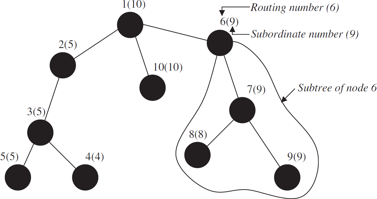
We define the routing number as the number that is assigned to a node in the preorder traversal phase. And this number acts as the address for the associated node. Beside this number, every node keeps another number called subordinate number, the largest assigned number that appears in the subtree of that node. For example, in Fig. 5, the node with routing number 6 bears the subordinate number 9 that appears as the largest number in the subtree of node 6. These two numbers (i.e., 6(9)) form the routing entity for the corresponding node. The pair 6(9) indicates that nodes with address 7–9 lie in the subtree of node 6. The routing number is shown as bare number whereas the subordinate number appears within the parentheses.

Figure 5.

Addressing of nodes with single level.

HN-Routing supports data routing based on the assigned addresses to the nodes. When the sink wants to send a packet to a specific destination sensor, it broadcasts the packet among its neighbors. Neighbor nodes receive the packet, and check whether the destination is within the subtree of the node. If the destination appears in the subtree, the node forwards the packet to its neighbors, otherwise it drops the packet. This forwarding repeats until the packet reaches the destination. The situation is shown in Fig. 6. The sink (1) wants to send a packet to node 8. The sink broadcasts the packet to its neighbors and node 2, 6, and 10 receive the packet. Then each node determines whether node 8 can be reachable via itself, i.e., node 8 resides in its subtree. The subtree of 2 contains nodes from 3-5, whereas node 10 contains only itself, but nodes 7–9 belong to the subtree of node 6. So node 6 takes the packet whereas the others drop it. Then, node 6 makes another broadcast and the packet is received by node 7. Finally the packet is received by node 8 at the next broadcast. When node 7 broadcasts the packet, it eventually reaches node 6 again, but at this time node 6 discards the packet.

Figure 6.

Routing packet to node 8 from the sink (dark lines show the path).

3.2. Hierarchical Numbering

A question arises, as to how many address bits are required to allocate address to the entire network? If we know (or guess roughly) about the size of the network (number of nodes), we can calculate the minimum number of bits to be [log₂(N)] for a network of size N. But in sensor applications, the number of nodes may not be known earlier or it may vary due to failure of nodes or addition of new nodes in the network. Keeping the address length arbitrarily large leads to underutilization of address bits against the network size, and it also increases the energy consumption due to a large address overhead in the packet. So the address allocation should adjust the address length according to the necessity of the network. This introduces the hierarchical levels in address.

The number assigned to the nodes is bounded by a value bpl, bits per level. If bpl is set to 3, the nodes can be numbered up to 7. Beyond this value, the node address takes multiple levels. In that case the address no longer remains in the form of a single whole number, say 5, rather it becomes something like 5.1 with two levels or 5.1.4 with three levels and so on. Bits per level (bpl) is a critical system parameter and is decided long before the sensors are deployed. For bpl = k, the largest number can appear in any level is 2^k − 1. When the number to be assigned is higher than the largest value in the current level, the address level is increased by one and the node takes the number from the next immediate level starting from 1. We name this phenomenon as hierarchical numbering. Hierarchical numbering comes into action when any node fails or new nodes arrive in the network.

In Fig. 7b, node H which gets number 4 in the single level allocation scheme, is assigned with address 3.1, an address of two levels. And similarly G is assigned with 3.2 in lieu of 5. Along with storing the routing and subordinate number as before, node E now keeps another number 2 as an auxiliary number that counts the number of nodes in the subtree of E that are assigned addresses in the next address level of E. Similar thing happens when node A goes for address allocation for node D. Node D takes address 1.1 and the other two nodes F and G in the subtree get addresses 1.2 and 1.3 respectively. Other two nodes C and J get addresses with three address levels. The auxiliary number of a node counts the number of nodes in the subtree that are assigned addresses in the next immediate level of the subtree root node. In multilevel addressing, the node address is represented as decimal octets with the last octet being the routing number whereas the subordinate number is shown in parentheses and the auxiliary number in the square bracket.

Figure 7.

Two address allocation schemes. (a) Single level. (b) Multiple levels for bpl = 2.

3.2.1. Data Routing with Hierarchical Levels

When addresses take hierarchical levels, the data packet is forwarded level by level. Suppose, in Fig. 7b, the sink A tries to send data to node G(3.2). Here the destination has two address levels, so two successive routing events are combined. First, data is forwarded to the node with address 3 (node E) which appears in the first address level of the destination. After node E is reached, routing is made onto the next address level. Now data is forwarded to node 3.2 and eventually reaches the destination G. Hence, the routing path is A → B → E → G. Therefore we can say that to reach a node, say 5.2.4.1, from the sink 1, the path to be followed is 1 → 5 → 5.2 → 5.2.4 → 5.2.4.1.

3.3. Address Allocation Technique

In this section, we narrate in details how addresses are assigned in HN-Routing. HN-Routing is a distributed message passing protocol where participant nodes pass message amongst themselves in order to find the spanning tree and assign labels on nodes in the preorder manner. We describe the allocation process with single level and with hierarchical levels separately.

3.3.1. Address Allocation with Single Level

The nodes are first organized into a tree structure rooted at the sink and then they are assigned addresses by their respective parent according to the preorder traversal of the tree. When a parent node starts allocating addresses to its children, it first picks one of its children (from a ready queue, as we will see subsequently) and assigns an address to it. The child node in turns assigns an address to its children, and it goes down to the leaves of the tree. Until a child has completely assigned addresses to all of the descendant children in the subtree, the parent node does not start the address allocation for the next child. In this way the preorder traversal of the tree is made and nodes are addressed one after another.

The sink node initiates the addressing process, and the protocol uses four control messages (actually six, we will describe other two later on) for address allocation:

ALERT: Node sends ALERT message to its neighbors, and the sink is the first node sending ALERT at the beginning. Upon receiving the ALERT message from any neighbor node for the first time, the recipient node selects the node from which it receives the ALERT message as the parent node and then forwards the ALERT message to its neighbors. Thus ALERT message propagates onto the network and a spanning tree is readily constructed.

READY: When a node selects its parent after receiving ALERT, it sends READY message back to the parent. When the parent gets the READY message back from its child, it puts the child's ID in the ready queue (if not inserted earlier). The ready queue is a list of child nodes that are candidates for address allocation by the parent.

NUMBER: The parent node picks one of the child nodes from the ready queue and sends a NUMBER message to it as a step of assigning an address to that child.

DONE: When a node is finished with assigning addresses to all of the nodes in its subtree, it sends the DONE message back to the parent. This DONE message makes the parent to send NUMBER message to another ready child and to initiate address allocation in the corresponding subtree.

In the course of address allocation, each node remains at any of the following four states:

NOT-NUMBERED: Initial state for all nodes except the sink. In this state, a node has not yet selected its parent and waits for an ALERT message to come from one of its neighbors.

READY: The node has selected its parent and now is ready to collect address from the parent.

NUMBERING: A node remains in this state if the address allocation of nodes in its subtree goes on. This state is initiated by the receipt of a NUMBER message from the parent. In this state, the parent picks a node from its ready queue, sends the NUMBER message to the node and waits for DONE message back from the same.

DONE: When a NUMBERING node gets its ready queue empty identifying that it has finished address allocation in all of its subtrees, it sends the DONE message back to the parent. Now its state becomes DONE and it remains here subsequently.

Numbering of nodes. Sink is the first node to be in the NUMBERING state and assigns its address as 1. Then it picks one of its children from the ready queue and sends NUMBER (k) message with k = 2 to that child. The value of k indicates that the descendant nodes beneath the parent node in the subtree are assigned a number starting from k. When a child node gets NUMBER (k) message from the parent, it switches to NUMBERING state (from READY) and assigns k as its routing number as well as its address. Then it picks one of its ready child from the ready queue (if there is any), sends NUMBER (k + 1) to the child and waits for the DONE message from the child. When the parent gets DONE(l) message from the child, it updates the value of k as k = l and picks the next child node from the ready queue and repeats the process by sending NUMBER(k + 1) to the child. If there is no child left in the ready queue, the node sends DONE(k) to its parent. The last value of k, that is returned to the parent by DONE(k), is stored as a subordinate number of the node. When a sink node gets the DONE message from all of its children, the address allocation for all nodes in the network is completed. The sequence of message passing and corresponding state update of nodes is presented in Fig. 8 for a small network.

Figure 8.

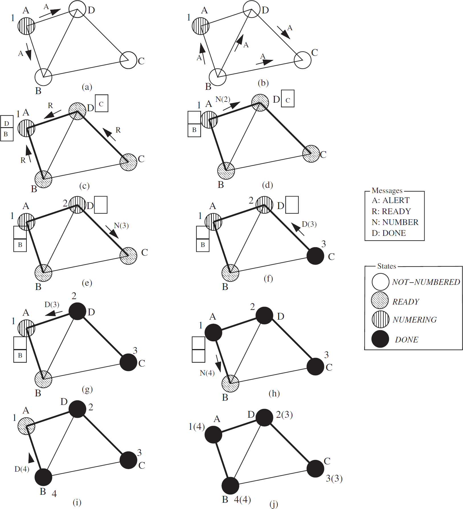
Sequence of message passing in address allocation of HN-Routing.

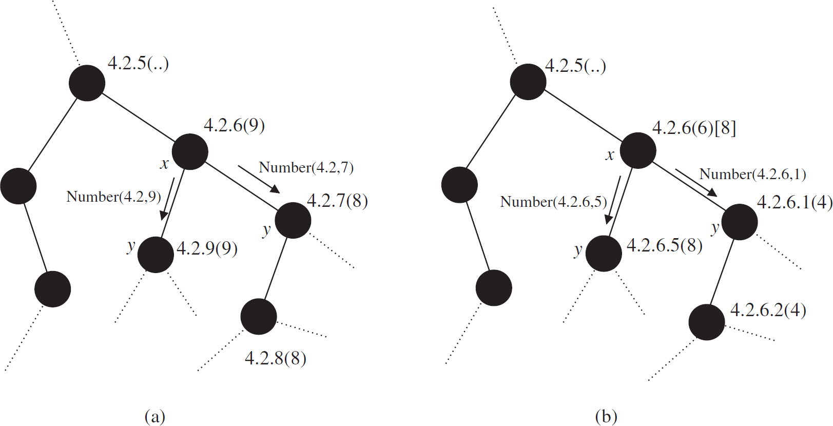
3.3.2. Address Allocation with Hierarchical Levels

When hierarchical address levels are incorporated, before sending the NUMBER(k + 1) message to a ready child, the parent node should check whether the next address assignment exceeds the largest number for the current level. If k < 2^bpl − 1, NUMBER(k + 1) is sent to the child node, otherwise the parent has to raise the address level by one. In the latter case, the parent switches to the next level addressing and issues a NUMBER(prefix, 1) message to the child where prefix is the address of the parent node. When the child receives the NUMBER(prefix, k) message, it appends prefix address with k to construct its own address. For single level address allocation, prefix address is null. When the parent node gets the DONE(l) message back from the child, two things can happen: if the parent node allocates addresses to subtree nodes in its current level (i.e., its last address level) it stores l as the subordinate number whereas if the parent were running it in the next level, it stores l as the auxiliary number.

3.4. Node Failure and Address Reallocation

Although HN-Routing involves the entire network at the initial phase of address allocation, it makes local adjustments when any node fails or a new node arrives. HN-Routing preserves a tree structure for its operation and failure of any node breaches the tree. HN-Routing's reallocation scheme restores the tree structure by finding a new parent for the affected nodes and reallocates new addresses for them quickly. If we are quite unlucky in getting one or more disconnected components due to node failure and the tree structure cannot be restored, we give up and there is hardly anything to do. Unless the network becomes disconnected from the sink, it can be shown that our reallocation approach works successfully. Nodes can fail at the time of address allocation phase or in the event sensing time.

3.4.1. Node Failure at Address Allocation Time

Since address allocation is done at the beginning of a network operation, it is safe to assume that nodes are full of battery power and rarely become dead or scheduled to sleep in that time. Still there may be failures due to catastrophic disorder of sensor radio or unexpected malfunction of circuitries inside the sensor body. Anyway, if any node fails, it may be in any of the four states namely NOT-NUMBERED, READY, NUMBERING, and DONE. Failure at DONE state actually corresponds to failure at the event sensing time.

Failure in NOT-NUMBERED state: If a node fails in a NOT-NUMBERED state before receiving any ALERT message, it makes no sense in our address allocation procedure. Address allocation completes smoothly leaving the dead node. If the node resumes later on, it can be treated as a new node and is handled separately.

Failure in READY state: In READY state, node selects its parent and sends READY message to the parent. Its ID is stored in the ready queue of its parent node for future address assignment. But if the node fails in this state, parent may not trace this failure. In the course of address assignment one child after another, parent node sends NUMBER message to this node and waits for a DONE message to be returned from it. Since the node is dead, it neither receives NUMBER message nor sends DONE. A DONE-TIMEOUT event is triggered and the parent leaves the child taking another child from its ready queue. If this dead node becomes alive at some future time, it becomes NOT-NUMBERED and obtains the address as a new node.

Failure in NUMBERING state: This case is pretty hazardous—ready queue is destroyed and no child gets the NUMBER message from the dead parent. After timeout the child leaves the parent, initiates the whole process by switching to NOT-NUMBERED state, and sends DISCARD-ADDRESS to all descendant nodes in the subtree. A dead NUMBERING node fails to send DONE message back to its parent, in that case the parent node is interrupted by a DONE-TIMEOUT event and proceeds to the next ready child. Figure 9 demonstrates such a scene.

Figure 9.

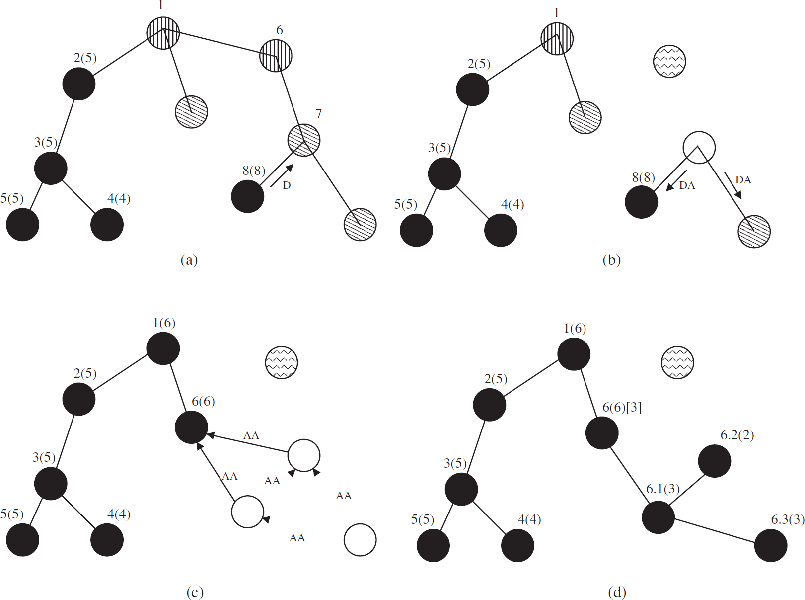
Reallocation of address due to node failure in NUMBERING state. (a) Node 6 fails, (b) Node 7 detects parent failure and sends DISCARD-ADDRESS to the child nodes, (c) sink timeouts for DONE from 6 and assigns address to another child, whereas the affected nodes leave their parent and seek address by ASSIGN-ADDRESS, and (d) nodes get addresses from 6.

3.4.2. Failure/New Node at Event Sensing Time

Whenever a node detects a dead parent, it discards its current address and tells the nodes in its subtree to discard their addresses by sending a DISCARD-ADDRESS message. Then, the affected nodes send a solicitation message ASSIGN-ADDRESS to their neighbors and eligible neighbor node that has not discarded its own address and has enough address space available (auxiliary number <2^bpl − 1) and initiates address reallocation by sending ALERT message to the affected node. The selected node becomes the new parent and the READY message is sent back to the parent. The parent now sends the NUMBER(prefix, k) message to the child where prefix is its own address and k = auxiliary number + 1. When the child returns DONE(l), the parent updates its auxiliary number as auxiliary number = l. Figure 10 shows such a reallocation scene. Sometimes the node goes to sleep for a while, and wakes up again. In that case, it may retain its earlier address by setting its subordinate number to routing number and auxiliary number to 0 (node 1.2 in Fig. 10).

Figure 10.

Reallocation of address. (a) Addressing for bpl = 2, (b) node 1.2 fails and children become orphan, (c) orphan nodes get address from 1.1.1, and (d) node 1.2 revives and adjusts its address.

When a new node is added to the network, it waits to hear an ALERT message from its neighbors. If any ALERT arrives, it participates in the allocation process, otherwise it sends ASSIGN-ADDRESS request to the neighbors. Eligible neighbors reply and the node is assigned an address (Fig. 11). Figure 12 shows the state diagram of the entire allocation process.

Figure 11.

Allocation of address for a new node. (a) Node sends ASSIGN-ADDRESS message to neighbors and (b) obtains address from 7.

Figure 12.

Transitions of states of node during address allocation. (Transition occurs upon the receipt of the labeled message.)

3.5. Address Parameters

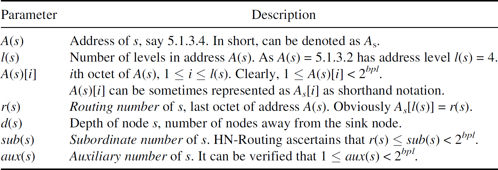
To analyze the routing scheme based on the assigned addresses to nodes we define the following address parameters for a sensor node s:

Parameter	Description
A(s)	Address of s, say 5.1.3.4. In short, can be denoted as A_s.
l(s)	Number of levels in address A(s). As A(s) = 5.1.3.2 has address level l(s) = 4.
A(s)[i]	ith octet of A(s), 1 ≤ i ≤ l(s). Clearly, 1 ≤ A(s)[i] < 2^bpl.
A(s)[i]	A(s)[i] can be sometimes represented as A_s[i] as shorthand notation.
r(s)	Routing number of s, last octet of address A(s). Obviously A_s[l(s)] = r(s).
d(s)	Depth of node s, number of nodes away from the sink node.
sub(s)	Subordinate number of s. HN-Routing ascertains that r(s) ≤ sub(s) < 2^bpl.
aux(s)	Auxiliary number of s. It can be verified that 1 ≤ aux(s) < 2^bpl.

Let us define a function match: Address × Address → Z⁺ which counts the largest prefix match in terms octets in two address. For example match(1.5.2.3, 1.5.4.2) gives 2 whereas match(6.2.1, 1.2) gives 0. The function match for address of two nodes x and y can be defined as:

m a t c h (A_{x}, A_{y}) = min {i : A_{x} [i] \neq A_{y} [i]} - 1 f o r 1 \leq i \leq max l (x), l (y))

If address are equal, i.e., A_x = A_y, then match(A_x, A_y) = l(x) = l(y).

We have the following properties on address parameters of nodes:

Property 3.1

If node x is the parent of node y, then d(y) = d(x) + 1.

Property 3.2

For any node y, l(y) ≤ d(y) + 1.

Property 3.3

If node x is the parent of node y, then l(y) = l(x) or l(y) = l(x) + 1.

Property 3.4 Detection of child

A node y is the child of node x (reversely, x is parent of y) if and only if d(y) = d(x) + 1 and any of the following two conditions is satisfied by then address parameters for m = match(A(x), A(y)):

l(x) = l(y) = m + 1 and r(x) < r(y) ≤ sub(x).

l(x) = l(y) − 1 = m and 1 ≤ r(y) ≤ aux(x).

Proof

The condition expressed by d(y) = d(x) + 1 is due to Property 3.1.

To prove the claim, we are to show that if x be the parent of y, any of the two conditions holds, and on the contrary if any of the two conditions holds, x should be the parent of y.

The proof is derived from two address allocation situations in HN-Routing. When a parent node assigns an address to one of its children by sending NUMBER message, one of two things can happen. Parent does assign number to the child in the last address level (if k < 2^bpl − 1) or increase the address level by one and assigns number in next address level. The proof can be constructed as follows for the two cases:

Case I. Addressing in the same level

Let x be the parent of y. In this case both x and y have the same number of address level. So l(x) = l(y). Since y receives address from x, a NUMBER (prefix, k) message is issued to y from x where prefix is the address of x without the last octet. Node y appends k after prefix to form its address. So A_x and A_y differs only in the last octet resulting m = match(A_x, A_y) = l(x) − 1. Again sub(x) denotes the maximum number that is obtained by any node in the subtree of x in the last address level of A(x), so y's routing number should lie within r(x) and sub(x). Hence we get r(x) < r(y) ≤ sub(x), and condition I is satisfied. Figure 14a shows the case.

Figure 13.

Various address parameters in HN-Routing.

Figure 14.

Demonstration of property 3.4. (a) Condition I: y gets address from x in the last address level. (b) Condition II: y gets address from x in the next address level.

Again, we assume l(x) = l(y) = m + 1 and r(x) < r(y) ≤ sub(x). We are to show that x is parent of y. Now, A(y) differs from A(x) exactly in the last octet and y's routing number lies within r(x) and sub(x). Again d(y) = d(x) + 1 makes y exactly one hop away from x. Hence y must have received address from x. So x is the parent node.

Case II. Addressing in next level

Let x be the parent of y. In this case, y has one more level in its address than x's and x's address is a complete prefix of y's address. So l(x) = l(y) − 1 and m = l(x). In our address allocation procedure y must have been assigned a number between 1 and aux(x) by the parent x and this number appears as y's routing number. So 1 ≤ r(y) ≤ aux(x). Figure 14b shows the scenario.

Again if 1 ≤ r(y) ≤ aux(x) holds and y's address has a complete prefix match with x (being m = l(y) − 1 = l(x)) and y is one hop away from x(d(y) = d(x) + 1), y must have taken address from x. So x is the parent of y. □

Due to Property 3.4, the parent node can determine its child from its address and similarly child nodes can determine their parent. As we see in Fig. 15, nodes can determine their parent depending on the address parameters of the nodes in the network.

Figure 15.

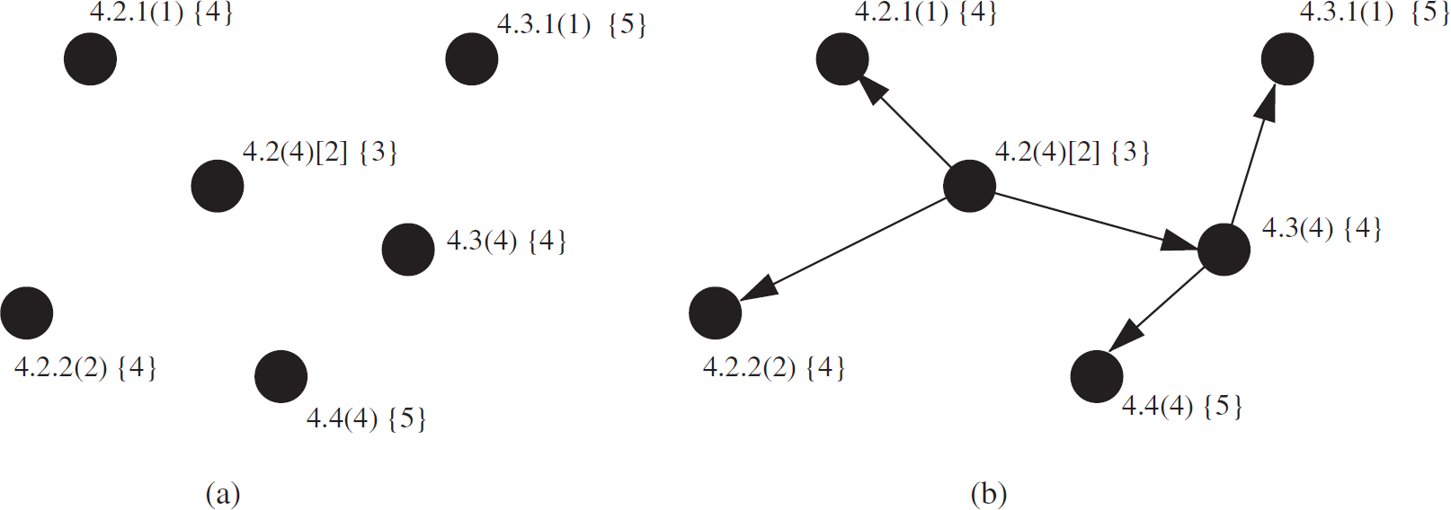
Detecting parent nodes: (a) bare nodes; (b) underlying tree (arrow directs from parent to child and number inside { } indicates depth).

Property 3.5 Detection of subtree node

For two nodes x and y with d(y) > d(x) and m = match (A_x, A_y), the node y lies in the subtree of x, if it satisfies any of the two following conditions:

m = l(x) − 1 and r(x) < A_y[m + 1] ≤ sub(x).

m = l(x) and 1 ≤ A_y[m + 1] ≤ aux(x).

Proof

The property directly follows from the address allocation technique. When a parent assigns an address to its children, it either assigns the address in its last address level or starts from 1 in the next address level. And this continues beneath the tree up to the leaves. Let x be the root of a subtree. Two cases can happen.

Case I. When the subtree nodes get the address of the same address level of x, their addresses differ only in the last octet and other octets are equal to A(x)'s. In this case, if y be a subtree node, we have m = match(A_x, A_y) = l(x) − 1. So A_y[m + 1] denotes the last octet in A_y. According to our addressing scheme this last octet is bounded by r(x) < A_y[m + 1] ≤ sub(x). When y in turn assigns an address to its children (y acts as parent) with a longer address level, additional octets are added after m + 1 level, keeping the first m address levels exactly same. Those nodes are also included in the subtree of x and condition I is satisfied for them.

Case II. When nodes are assigned an address with one additional address level of their parent, they take a new level and their addresses exactly match with the parent in all octets except the last. The number in the additional address level is bounded by the auxiliary number of the parent. If x be a parent and y be a subtree node, we have m = match(A_x, A_y) = l(x). So A_y[m + 1] denotes number in the additional address level and is bounded by 1 ≤ A_y[m + 1] ≤ aux(x). When this y assigns addresses to nodes with longer address levels, those nodes also appear in the subtree of x and condition II holds for them too. □

Due to the Property 3.5, any node can determine whether a destination node resides in its subtree by examining the destination address (Figure 16). In that case, the node participates in forwarding of the packet en-route to the destination. This is how HN-Routing makes stateless routing based on assigned address.

Figure 16.

Illustration of Property 3.5. (a) The possible subtree nodes. (b) Possible nodes in the subtree of 1.4.3(5)[2].

Corollary 3.1

Node y is a child of node x if and only if y lies in the subtree of x and y lies one hop away from x, i.e., d(y) = d(x) + 1.

4. Routing Rules of HN-Routing

In this section we describe the types of packets we consider in the sensor network and we present routing rules for them in the context of our proposed addressing scheme. We define three types of packets:

(I)
Request packet: Sometimes the sink passes some specific control data to any specific sensor node. Request packet p contains following fields:
D(p): Address of the destination node to which request is to be reached.

d(p): Depth of packet forwarder node. This field is updated each time the packet is forwarded by a node.

data(p): Requested data of interest.

It is seen that request packet does not contain the sender address, because sender is implicitly the sink.
(II)
Response packet: In response to the sink's query on any specific event, a node can send response packets to the sink if it gathers relevant data of the queried event. In the application of periodic observation, sensors might send a response packet with their observed data to the sink without the prior query from the sink. The response packet contains:
S(p): Address of the node that generates the response packet destined to the sink.

d(p): Depth of packet forwarder node. This field is updated each time the packet forwarded by a node.

data(p): Response data of the observed event.

Here packet does not contain the destination address, because destination is implicitly the sink.
(III)
Query packet: This packet is issued by the sink node and is flooded into the entire network. All nodes should receive the packet and forward it accordingly. It contains:
A(p): Address of the forwarder node of the query. Initially it is sink's address.

sub(p): Subordinate number of the forwarder node of the query packet.

aux(p): Auxiliary number of the forwarder node of the query packet.

d(p): Depth of the forwarder node.

query(p): Query data of interest.

Query packet contains neither the sender nor the destination address, rather it contains the address of the intermittent node that passes the packet onward. The sink is the sender and all nodes in the network are the receiver.
4.1. Routing Rules

Below we discuss the routing rules of HN-Routing for the above three types of packets.

Request Packet: The request packet p is constructed by the sink by setting packet fields as D(p) = destination address, d(p) = 0 and data(p) = control data to pass.

Routing Rule: Request Packet at [Node x]

Receive (Request p) /∗ When a Request packet is received, do following. ∗/

If (D(p) = A(p)) /∗ Check whether destination is reached. ∗/

- Accept and record p; /∗ Destination is reached. ∗/

Else If (d(x) = d(p) + 1 and D(p) lies in the subtree of x)

/∗ The reason for checking depth is to restrict the broadcast in the same level. ∗/

/∗ This prevents the immediate sender to receive the packet back. ∗/

- Accept p;

- Set d(p) = d(x), keep other packet fields unchanged; /∗ Depth is updated. ∗/

- Broadcast p to neighbors;

Else

Drop p; /∗ Neither it itself is destination nor the destination is in the subtree. ∗/

End Rule

Response Packet: Any sensor node prepares the response packet p by putting packet fields as S(p) = node address, d(p) = depth of the node and data(p) = event data to be passed to the sink. We build the following routing rule for this sort of packet.

Routing Rule: Response Packet at [Node x]

Receive (Response p)

If (x = sink)/_∗ Whether the node is the sink itself ∗/

The sink is reached;

Accept and record p;

Else If (d(x) = d(p) −1 and S(p) lies in the subtree of x)

/∗ Packet is going backward, hence the depth is checked accordingly ∗/

/∗ The sender S(p) should lie in the subtree of the recipient x ∗/

Accept p;

Set d(p) = d(x), keep other packet fields unchanged; /∗ Depth is updated ∗/

Broadcast p to neighbors;

Else

Drop p;

End Rule

Query Packet: A query q is constructed by the sink with the packet fields as A(q) = A(sink), sub(q) = sub(sink), aux(q) = aux(sink) and d(q) = 0 and arbitrary query data of interest as query(q). For a node x, we can have the following query routing rule.

Routing Rule: Query Packet at [Node x]

Receive (Query q)

If (node A(q) is the parent of x) /∗ Query is sent by the parent node ∗/

Accept and record q;

/∗ Whenever query packet changes the hop, the packet contains the address of intermittent node ∗/

Set A(q) = A(x), sub(q) = sub(x), aux(q) = aux(x) and d(q) = d(x);

Broadcast q to neighbors;

Else

Drop q; /∗ Packet does not arrive from the parent ∗/

End Rule

Now we produce a formal proof of correctness of the proposed routing scheme based on properties 3.4 and 3.5.

Lemma 4.1

According to the routing rules, data packets can be routed to specific destination from the sink and vice versa.

Proof

Let, the sink send a request packet to the destination node d. Let A(d) = a₁.a₂. · · · .a_n and d(d) = k. According to our routing principle, the packet is routed along a path of nodes v₁ v₂ · · · v_k in the tree such that v₁ = sink, v_k = d and node d lies in the subtree of every v_i in the path for 2 ≤ i ≤ k − 1. We show that such a path exists in the tree.

For multilevel addresses, we forward the data packet level by level. So the data is routed along routes as 1 ⇝a₁, a₁ ⇝a₁ .a₂, a₁ .a₂⇝a₁ .a₂ .a₃ and at last a₁ .a₂. · · · .a_n-1 ⇝a₁ .a₂. · · · .a_n. To exist a path to the destination from the sink, every intermediate nodes a₁, a₁ .a₂, · · ·, a₁ .a₂. · · · .a_n-1 must exist. We can verify that they exist. According to the addressing scheme, a₁ .a₂. · · · .a_i+1 lies in the subtree of a₁ .a₂. ··· .a_i. If i fails, all nodes in the subtree would discard their address (by DISCARD-ADDRESS message) and they all will be reallocated newer addresses by other nodes (by ASSIGN-ADDRESS).

Let x be the node with address A(x) = a₁ .a₂ · · · a_i and y be the node with address A(y) = a₁ .a₂. · · · .a_i+1. Now we show that a single path exists from x to y. Before this, we are supposed to show that path 1⇝a₁ exists, but this is trivially observed from the description that follows.

Node y lies in the subtree of x and according to the Property 3.5 we have 1 ≤ r(y) ≤ aux(x). Without loss of generality let us assume that x has exactly two children u and v. If any of u and v be the node y, a path exists between x and y and we are done.

If neither u nor v be the node y, then the node y must lie in the subtree of either u or v. Let node u gets its address from x first, and then v gets. According to the addressing scheme, r(u) = 1, r(v) = sub(u) + 1, sub(v) = aux(x) and r(y) = a_i+1. Let y lie in the subtree of u. Since the address of u and y differ only in the last octet, according to the property 3.5, r(u) < r(y) ≤ sub(u), i.e., 1 < a_i+1 ≤ sub(u). Since u and v allocate addresses to their descendant children (Fig. 17) in two disjoint intervals, y has no way to lie in the subtree of both u and v at the same time. In the same way, if y lies in the subtree of v, it cannot lie in the subtree of u either. So we get a single edge en-route to y from x. Similarly, other edges can be found beneath node u to reach y that leads a single path to node y from x.

Figure 17.

Detecting path along the tree en-route to a destination.

So, a single path exists between 1⇝a₁, a₁⇝a₁ .a₂, and at last a₁ .a₂. · · · .a_n-1 ⇝a₁ .a₂. · · · .a_n.

Therefore, data packet can be routed to the destination node d from the sink.

Response packet does the reverse operation of request packet. So packet can be routed from any sensor node to sink. □

5. Simulation Results

In this section we describe the simulation results of HN-Routing. The main objective of the simulation is to understand the impact of various parameters on the performance of the protocol. We also simulate TreeCast to make a comparison between our approach and TreeCast on various metrics.

5.1. Simulation Setting

We simulate HN-Routing using PARSEC [2], a C-based parallel discrete event simulation language. Table 1 presents the entire simulation setting.

Table 1
Simulation Setting

Parameter Value

General Settings

Target area 1000m × 1000m

Number of nodes (N) 50-300

Usual number of nodes 200

Sink location (500, 500)

Transmission radius (R) 125 m

Node density μ(R) 10 (Approx.)

Bits per level (bpl) 3-10

Number of runs 5

Channel Characteristics

Propagation model Friis free space (r² path loss)

Signal transmission range Fixed (125m)

Channel Symmetric

Energy Consumption

Radio model First order radio model

Energy for transmitter electronics (E_Tx-elec) 50 nJ/bit

Energy for receiver electronics (E_Rx—elec) 50 nJ/bit

Energy for transmitter amplifier (∈_amp) 100 pJ/bit/m²

Energy/bit ≈ 1.56 J/bit

Event Reporting

Reporting type Discrete event-driven

Packet type Request, Response, Query

Event generation process Poisson

Inter-arrival of events Exponential (mean 1000 STU*)

Event generator node selection Uniform random

Total packet transmission 100

Data length in packet 16 bits

Node Failure Model

Failure model Continuous and consecutive

Time gap between two failures (continuous) Exponential (mean 1000 STU)

Sleeping time (consecutive) Exponential (mean 100 STU)

Failing node selection Uniform random

Parameter	Value
General Settings
Target area	1000m × 1000m
Number of nodes (N)	50-300
Usual number of nodes	200
Sink location	(500, 500)
Transmission radius (R)	125 m
Node density μ(R)	10 (Approx.)
Bits per level (bpl)	3-10
Number of runs	5
Channel Characteristics
Propagation model	Friis free space (r² path loss)
Signal transmission range	Fixed (125m)
Channel	Symmetric
Energy Consumption
Radio model	First order radio model
Energy for transmitter electronics (E_Tx-elec)	50 nJ/bit
Energy for receiver electronics (E_Rx—elec)	50 nJ/bit
Energy for transmitter amplifier (∈_amp)	100 pJ/bit/m²
Energy/bit	≈ 1.56 J/bit
Event Reporting
Reporting type	Discrete event-driven
Packet type	Request, Response, Query
Event generation process	Poisson
Inter-arrival of events	Exponential (mean 1000 STU*)
Event generator node selection	Uniform random
Total packet transmission	100
Data length in packet	16 bits
Node Failure Model
Failure model	Continuous and consecutive
Time gap between two failures (continuous)	Exponential (mean 1000 STU)
Sleeping time (consecutive)	Exponential (mean 100 STU)
Failing node selection	Uniform random

STU means Simulation Time Unit.

Simulation environment and parameters: We run our simulation for sensor networks of size 100–500 nodes which are placed uniformly in a two dimensional area of 1000 m × 1000 m. We usually keep the number of sensor nodes to 200 (due to TreeCast [23]), when the performance is evaluated against the parameter other than the network size. If not otherwise specified, we assume the location of the sink is in the center of the scene at (500, 500). Each node is assumed to have a transmission radius of 125 m. This gives node density to be $\frac{200}{1000 \times 1000} \times (π \times 125^{2}) \approx 10$ nodes per transmission area. For computing average values, we run the simulation five times with the same setting, but with different scenes of node deployment.

Energy consumption model: In our simulation, we consider the first order radio model for the sensor radio (Fig. 18), as suggested in [10]. We consider the energy consumption due to data communication only, no power consumption for data processing is considered.

Figure 18.

First order radio model for sensor node.

In the first order radio model, to transmit a k-bit message to a distance of d, energy dissipation by the radio is given by:

E_{T x} (k, d) = E_{T x - e l e c} (k) + E_{T x - a m p} (k, d) = E_{e l e c} \times k + ϵ_{a m p} \times k \times d^{2}

and to receive the message of the same length, the radio expends:

E_{R x} (k, d) = E_{R x - e l e c} (k) = E_{e l e c} \times k

Detailed technical treatment of this radio model is due to [9]. According to the values appeared in Table 1, a sensor node takes nearly 1.56J to transmit a single bit to 125 m away.⁴

Event reporting: In the sensor applications, two types of event reporting can be possible [10]: continuous and discrete. In the continuous reporting, sensors periodically send their observed data to the sink in some regular interval, and it usually happens when sensors are deployed to observe some ambient condition of the target environment. But in discrete reporting, sensors send data to the sink whenever a certain event has occurred in the sensing area and the sensor detects it. In our simulation we conduct a discrete event-driven data reporting technique which is modeled by a Poisson process with the mean inter-arrival time of 1000 unit of simulation time.

Failure model: We consider only node failure and ignore link failure. We also assume that nodes are of infinite frame buffer and no packets are ever lost in the channel. We adopt two types of node failures: continuous and consecutive. In the continuous failure, node fails and never resumes later, but in the consecutive failure node goes to sleep shutting down its radio and remains inactive for a while, and wakes up asynchronously later on.

Performance metrics: The performance metrics that we consider in our simulation are message cost for addressing, address length, communication energy, packet latency, and delivery rate. Message cost for addressing is the number of messages required to assign addresses to all nodes. Address length is the average address length in bits that is assigned to nodes in address allocation phase. Another performance metric is communication energy that measures the total energy dissipated by sensors in sending and receiving data packets. Simulation shows the impact of the address length on packet communication. Packet latency measures the time taken by the packets to reach the sink, whereas the delivery rate shows the fraction of packets delivered to the sink with respect to the total packets sent.

5.2. Performance Evaluation of HN-Routing

In the simulation, we vary the number of nodes (N) and bits per level (bpl) to observe the behavior of performance metrics. To limit the illustrations, we depict only some particular simulation-based scenarios where subtle changes in various parameters (e.g., number of nodes, bits per level, etc.) result in salient differences in the performance. We also consider the failure of nodes and evaluate the performance thereafter accordingly.

5.2.1. Tree Formation

The HN-Routing protocol organizes sensor nodes in a tree structure rooted by the sink. Figure 19 shows a scene of 200 nodes. To show explicitly the quality of the tree formed by the algorithm, we produce Fig. 20 which shows the depth of the nodes in the tree against the Euclidean distance of nodes from the sink. It shows that most of the nodes are in the smallest depth in accordance with the distance from the sink. Sometimes nodes do receive address allocation messages from the neighbor of higher depth rather than the one of lower depth. This makes multiple depths to exist at the same distance for different nodes (e.g., at a distance of 500 m from the sink).

Figure 19.

Scenario of 200 nodes in 1000 m × 1000 m area. (a) Nodes are scattered randomly in the area. (b) Generated tree for the scene (squared node is the sink).

Figure 20.

Depth of nodes against the distance from the sink.

5.2.2. Message Cost for Addressing

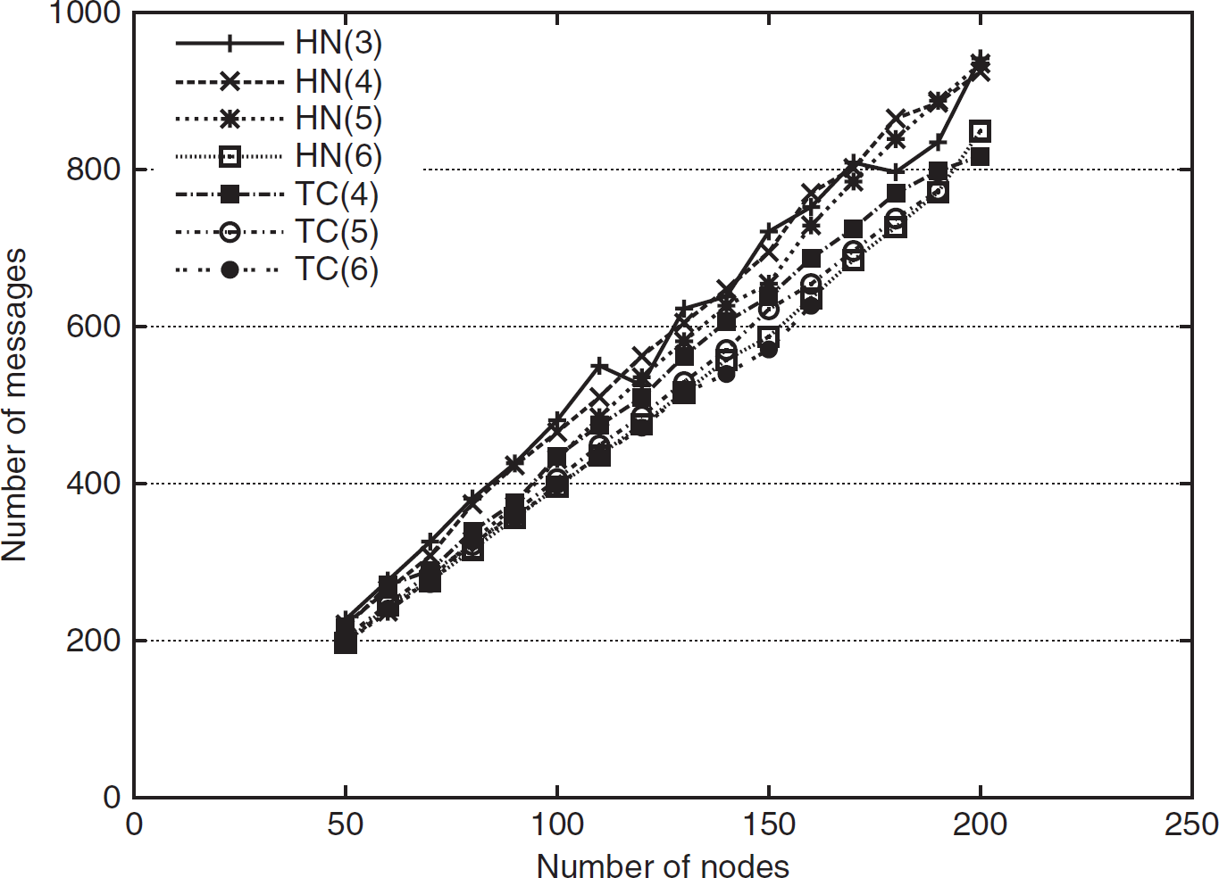
Figure 21 shows the message count for addressing by HN-Routing. As Fig. 21 reveals the message cost for the addressing of nodes is nearly four times the number of total nodes. This count is due to the fact that if no node ever fails and all events go smooth, every node sends ALERT, READY, and DONE messages exactly once and receives the NUMBER message once. Fewer messages are exchanged due to the READY-TIMEOUT event occurred when a READY child does not get the NUMBER message in time.

Figure 21.

Message cost for addressing in HN-Routing. HN(x) indicates HN-Routing with bpl = x.

The value of bpl has an impact on the message count. Parent nodes sometimes run out of all available numbers when the auxiliary number reaches its maximum value (shown in Fig. 22), and this causes the affected nodes adjust their parent by passing extra messages. This happens more frequently for smaller value of bpl.

Figure 22.

Parent adjustment. (a) Parent 2.1 cannot give address to one of its child node; (b) child changes the parent and gets address 2.1.2.1 from 2.1.2.

5.2.3. Address Length

Address length is the principal performance metric in our simulation. We compute the average address length as obtained by the nodes in the network, as follows:

A v e r a g e a d d r e s s l e n g t h = \frac{1}{N} \sum_{x} (l (x) \times b p l) bits

where l(x) is the number of address level of node x and N is the number of total nodes in the network.

Node distribution against depth/level In Fig. 23, we show the depth/level wise distribution of 200 nodes for bpl = 3 and bpl = 5 for the scenario in Fig. 19. The bar chart unveils that the distribution of nodes against the level is somewhat left skewed than that against the depth, and with the rise of value of bpl node distribution becomes more skewed to the left. It also shows that for a larger value of bpl, more nodes get smaller number of address levels, resulting in a reduction of the average address length.

Figure 23.

Depth vs. Level for 200 nodes. (a) bpl = 3, (b) bpl = 5.

Impact of bits per level The value of bpl has a subtle impact on the average address length. Higher bpl value makes the address length longer, but it does accommodate more sensor nodes in the same address level, resulting in a fewer number of address levels. On the other hand, smaller bpl value makes the address length shorter, but fewer number of nodes can be allocated in the same address level requiring a higher number of address levels. It is hard to predict what value of bpl makes the overall address length minimum.

Figure 24 demonstrates the impact of bpl on the average address length for a network of size 50–300 nodes. We list the following observations regarding the impact of bpl on the average address length.

For a smaller value of bpl, say 3 or 4, the address length is quite high for any size of network.

As bpl rises, address length gradually declines and at some point it gets the minimum value, then again it goes up. The value at which the address length obtains its minimum value is somewhat near to ⌈log₂(N)⌉. A network of size N requires at least ⌈log₂(N)⌉ bits to address all nodes in a single address level. For example, a network with 50 nodes achieves the minimum address length at bpl = 6, whereas a network with 300 nodes gets at bpl = 9.

When bpl > ⌈log₂(N)⌉, address becomes longer and consistently climbs up thereafter (upward tail in Fig. 24). In this case, hierarchical levels occur quite seldom and almost all addresses are in the very single level producing the address length to be equal to bpl. Very few nodes may take multiple levels that makes the address length slightly greater than bpl.

Experiment shows that addresses with multiple levels do not necessarily decrease the address length. Addressing requires minimum space if a single level is created, and then the address length becomes fixed by ⌈log₂(N)⌉. But the addressing scheme with multiple levels is a must because we cannot be sure about the number of nodes in advance in the sensor application. Moreover, address reallocation in case of failure of nodes requires multiple address levels.

Figure 24.

Impact of bits per level (bpl) on average address length on varying network size. The figure on the right side is for network size 200.

5.2.4. Communication Energy

We make the following assumptions in our simulation to analyze the communication energy:

Fixed data length. We assume that all data packets (query, request, or response) contain data of length 16 bits. In fact any size of data length can be assumed, but in order to trace the impact the address overhead precisely (to compare the observation against TreeCast as well), we consider constant data length rather than choosing it randomly.

Packet formation. The packets are formed with the fields as shown in Fig. 25. We assume that the depth and the number of levels are 4-bit numbers allowing a total of 16 depth values and 15 address levels which are quite sufficient for a network smaller than 1000 nodes deployed in 1000 m × 1000 m. In our experiments, we do not have any depth/level value greater than 16. For large scale deployment, these fields can have few more bits.

Figure 25.

Packet fields of HN-Routing (field lengths are measured in bits).

In the simulation we select an active node randomly and make it send a response packet to the sink. Since the content of both the request and the response packet is the same and they follow the same route to the target, we consider only the response packet. We generate 100 such events for a specific sensor deployment and get an average over them. To get the final average value of the energy, we take an average of 5 observations from 5 different scenes. The simulation output is shown in Fig. 26.

Figure 26.

Energy consumption of packet routing in HN-Routing for different bpl and network size.

We can list the following observations regarding energy consumption curve as shown in Fig. 26.

The optimal value of bpl to minimize the energy/packet and average address length are the same as energy is proportional to the address length. So the observations regarding the impact of bpl on the average address length is also applicable in case of the energy/packet.

Network size has some, though little and somewhat irregular, impact on the energy/packet. Major contributions in communication energy are due to the address length and the depth of nodes. As nodes are uniformly deployed in the area, distribution of nodes against depth may remain quite similar for varying network size. But the average address length of nodes becomes slightly longer for a larger network. The value of bpl plays an intricate impact on energy/packet against the network size. Smaller network may not be able to make complete utilization of address bits at all levels, whereas a larger network can make better usage of address bits by optimal selection of bpl.

The position of sink has an important impact on energy/packet. In Fig. 26(right) we show the energy consumption for 200 nodes against the four positions of sink at (500, 500), (333, 333), (250, 250), and (200, 200). For the position at (500, 500), the sink is located at the center of the network. In this case, nodes are at minimal depth compared to other positions of the sink. Hence, at (500, 500) we get the minimum energy curve. As the sink shifts away from the center to the corner, the depth of nodes as well as the energy/packet rises. However, in each position of the sink, individual energy curve shows the identical trend against bpl, getting the minimum value at bpl = 8.

5.2.5. Latency and Delivery Rate

The performance of HN-Routing in terms of packet latency and delivery rate is shown in Fig. 27 for a network of 200 nodes. In the latency curve, we plot the average delay to reach the sink against the hop distance from the sink. We normalized the delay with respect to the time required to pass a single hop. We plot two curves, one with zero node failure and another with 20% node failure. As we observe, when the failure of nodes occurs, latency rises and deeper nodes suffer greater latency.

Figure 27.

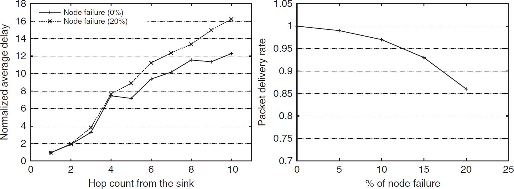
Latency and delivery rate of HN-Routing.

Again, it is evident from the operation of HN-Routing that a packet never fails (unlike other greedy geo-routing) to reach the sink if the network is connected with the underlying tree structure and all nodes are properly addressed. Moreover, there is no chance that a packet is routed along a wrong path. When a node fails, some nodes have to restore their addresses, and in the meantime all packets forwarded to them are dropped. If routing events are made synchronous with address adjustment (i.e., nodes send data only when they are stable with their addresses), the success rate can be made 100%. Moreover, when more and more nodes fail (as for 20% of nodes), the network tends to become disconnected from the sink, hence the delivery rate gradually decreases. But this failure should not be attributed to the routing protocol since no routing scheme can forward data between two disconnected components.

5.2.6. Performance on Node Failure

HN-Routing uses the address reallocation approach in case of node failure. As the node fails, the address length may increase because new addresses are sometimes allocated by raising the address level. Simulation observations are presented in Fig. 28 for both continuous and consecutive failure of nodes. In each failure model, we make 20% nodes to fail randomly one after another keeping a random time gap between two successive failures. In Fig. 28, we show the effects for three independent simulation runs on the same network (200 nodes) with three different sets of failed nodes. The curves indicate that the address length does not deteroriate very much in case of node failure and the address length roams around the initial allocation curve. However, in case of consecutive failure the address length is slightly worse than continuous failure.

Figure 28.

Average address length against node depth in case of node failure. (a) Continuous failure; (b) consecutive failure.

5.3. Comparison with TreeCast

In this section, we make a comparison between our HN-Routing with TreeCast based on several performance metrics.

5.3.1. Message Cost for Addressing

Both HN-Routing and TreeCast use distributed message passing technique to allocate addresses to nodes in the network. TreeCast uses four types of messages namely ALLOCATE, APPROVE, COMPLAINT, and CONFIRM in its address allocation phase [23]. HN-Routing also passes four types of messages like ALERT, READY, NUMBER, and DONE in its addressing process. HN-Routing also passes two other messages ASSIGN-ADDRESS and DISCARD-ADDRESS to tackle the failure of nodes in the middle of address allocation process. Figure 29 presents the simulation output of the initial message cost for addressing in both the schemes. The figure reveals that HN-Routing takes slightly more messages than TreeCast keeping the trend exactly the same. In both the cases, the message count is approximately four times of the network size.

Figure 29.

Initial message cost for address allocation in HN-Routing and TreeCast.

5.3.2. Average Address Length

Unlike TreeCast, HN-Routing does not increase the address level at every depth of the tree, rather it utilizes all addresses in certain address levels bounded by the bits per level (bpl) and switches to the next address level when all addresses in a certain level are exhausted. This makes better utilization of address bits by HN-Routing and average address length of nodes is smaller than that of TreeCast.

Regarding the address length, HN-Routing outperforms TreeCast by a big margin. Figure 30 shows the simulation result for 200 nodes in this regard. As the bar chart indicates, with the increase of bpl, HN-Routing gradually reduces the address bits whereas TreeCast grows it up constantly. In Fig. 30, we show the average address length for 200 nodes by varying bpl from 3 to 7. No TreeCast observation has been found for bpl value 3, because by setting bpl value to 3, we limit the number of children of a parent node to be at most 7 (= 2³ − 1). As we are running our simulation for the node density 10, there may be nodes that cannot be assigned addresses from their parents due to running out of all possible addresses. So, we left the bar empty for TreeCast in that case. It is also observed that the minimum address length of TreeCast is much higher than the maximum value of HN-Routing within the observed range of bpl.

Figure 30.

Average address length in HN-Routing and TreeCast.

5.3.3. Communication Energy

We compare our proposed routing technique against TreeCast in terms of energy consumptions in routing events. Since the data field is fixed, the address length plays the dominating role in energy dissipation by the senors in packet sending and receiving. In Fig. 31, we show the average energy consumption per packet for the response packet to the sink. The bar chart demonstrates that in terms of energy per packet HN-Routing is far better than TreeCast. This is due to the following two facts:

HN-Routing keeps address length shorter and hence reduces the address overhead in the data packet resulting to a reduction in communication energy. But in case of TreeCast, the address length is much longer than HN-Routing which makes energy consumption per packet greater.

What makes TreeCast worse is that in TreeCast with the increase of depth (or level), node address gets longer. A node far away from the sink with a larger depth value is assigned an address with an address level equal to its depth which makes the address length much longer. Therefore, long addresses are to traverse a long way to reach the sink and vice versa. This contributes a double impact on energy/packet (longer address passes more hops) that makes the communication energy quite large. And with the increase of bpl, TreeCast raises the address length and hence the energy/packet along the way.

Figure 31.

Energy/packet for HN-Routing and TreeCast.

5.3.4. Address Allocation Time

This metric measures how much time the addressing protocol takes to assign an address to all nodes in the network. The simulation result is shown in Fig. 32. It depicts that HN-Routing is worse than TreeCast in this metric. TreeCast assigns addresses to the entire network much faster than HN-Routing.

Figure 32.

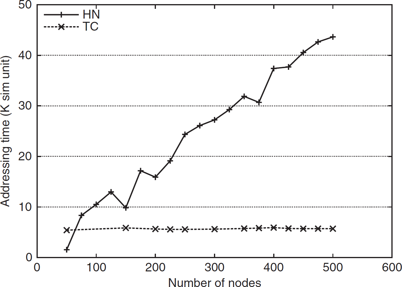
Address allocation time for a network of size 200 with bpl =5.

A longer time requirement of HN-Routing to allocate the address to all nodes is due to the fact that HN-Routing assigns the address to each node consecutively, one node at a time. But in TreeCast, several nodes can actively participate in the address allocation process at the same time. When a node is confirmed with its own address, it can safely go for addressing of the nodes in its subtree. So address allocation in subtrees can go in parallel, whereas in case of HN-Routing, only after finishing address allocation to all nodes in a subtree, a parent node can go for another child. So no simultaneous allocation process among the subtrees is possible (Fig. 33). TreeCast takes allocation time in the order of the depth of the tree, whereas HN-Routing takes time in the order of the number of nodes. Although, HN-Routing takes longer time during the initial address allocation phase, it saves lots of energy spent in event reporting that will run almost the entire life of the network.

Figure 33.

Address allocation. (a) HN-Routing: address allocation is going on in subtree A under x, until node x returns DONE(l) message to its parent, no node in subtree B under node y can have address. (b) TreeCast: if both x and y are approved with their addresses, both subtree A and B can be active in address allocation.

5.3.5. Summary

In comparison between HN-Routing and TreeCast, we can draw a summary as shown in Table 2.

TABLE 2
Summary of comparison between HN-Routing and TreeCast

Parameter HN-Routing TreeCast

Message count Nearly 4 × N Nearly 4 × N

Address length Good (logarithmic) Poor (Linear)

Data routing Yes Yes

Packet overhead Small Large

Handling node failure Adjust address Alternate Route

Communication energy Better Worse

Addressing Time Poor (Linear) Good (Logarithmic)

Parameter	HN-Routing	TreeCast
Message count	Nearly 4 × N	Nearly 4 × N
Address length	Good (logarithmic)	Poor (Linear)
Data routing	Yes	Yes
Packet overhead	Small	Large
Handling node failure	Adjust address	Alternate Route
Communication energy	Better	Worse
Addressing Time	Poor (Linear)	Good (Logarithmic)

6. Conclusion and Future Works

Sensor network is a very hot research topic in recent years. Addressing and routing are two important networking aspects of any network. Due to energy and other physical constraints of sensors, these two affairs differ significantly for sensor network from other networks. In this paper, we propose a new stateless addressing and routing scheme for wireless sensor networks. Apart from the cost for the initial address setup phase, this approach can perform better in terms of energy consumption in event reporting than the other geo-routing technique, especially when sensors are deployed in the indoor environment.

The approach can be investigated for further improvement. A more energy-efficient addressing technique can be investigated by introducing shorter length addresses for furthest nodes from the sink and relatively longer addresses for nodes closer to the sink. This would reduce the overall address overhead in communication. Moreover, instead of using hierarchical (multiple) levels for supporting failure/addition of nodes, one may try to find a clever scheme that uses only a single level to set the label on nodes and handles all of these. This will be a great breakthrough in the current task. Incorporating some energy-saving techniques (like sleep-awake based on some schedule) in the current scheme can be also thought about. Again the impact of mobility of nodes or the sink can also be investigated. Data aggregation on the proposed routing scheme can be another good research issue. The authors are focusing on the last issue (aggregation) in their future work.

Footnotes

1

In some literature, it is named as geometric routing, classified as geographic, location-based, position based, or simply geo-routing.

2

For a unit disk tree in grid of size n nodes, it requires at least (√n+9/12)² anchors [].

3

We set a label on nodes by assigning a number on them and this label acts as the address for that node. In this paper, we use the term “address” and “label” of nodes interchangeably.

4

$E = E_{e l e c} + ϵ_{a m p} \times d^{2} = 50 \times 10^{- 9} + 100 \times 10^{- 6} \times 125^{2} \approx \frac{125^{2}}{10^{4}} \approx 1.56 J$

References

Al-Karaki

J. N.

Kamal

A. E.

, “Routing techniques in wireless sensor networks: A survey,” IEEE Wireless Communications, vol. 11, pp. 6–28, December 2004.

Bagrodia

Meyerr

Takai

Chen

Y. -A.

Zeng

Martin

Song

H. Y.

, “PARSEC: A parallel simulation environment for complex system,” Tech. Report, UCLA, 1997.

Bose

Morin

Stojmenovic

Urrutia

“Routing with guaranteed delivery in ad-hoc wireless networks,”

ACM Wireless Networks, pages 609–616, November 2001, New York, USA.

Dohertry

Ghaoui

L. E.

Piste

, “Convex position estimation in wireless sensor networks,” in Proc. of Joint Conference of IEEE Computer and Communications Societies (INFOCOM), 2001.

Dunkels

Alonso

J. J.

Voigt

Ritter

Schiller

, “Connecting wireless sensornets with TCP/IP,” in International Conference on Wired/Wireless Internet Communication (WWIC), 2005.

Dunkels

Voigt

, “Making TCP/IP viable for wireless sensor networks,” in Proc.of the First European Workshop on Wireless Sensor Networks (EWSN), 2004.

Finn

G. G.

, “Routing and addressing problems in large metropolitan-scale internetworks,” Tech. Report ISi/RR-87–180, ISI, March 1987.

Gao

Guibas

L. J.

Hershburger

Zhang

Zhu

, “Geometric spanner for routing in mobile networks,” in Proc. of the 2nd ACM Symposium on Mobile Ad Hoc Networking and Computing (MobiHoc2001), pages 45–55, October 2001.

Heinzelman

, “Application-specific protocots architecture for wireless networks,” PhD dissertation, MIT, June 2000.

10.

Heinzelman

Chandrakasan

Balakrishnan

, “Energy-efficient communication protocols for wireless microsensor networks,” in Proc. of the 33rd Hawaii International Conference on System Sciences (HICSS ′00), pages 2–10, January 2000.

11.

Heinzehman

Kulik

Balakrishnan

, “Adaptive protocols for information dissemination in wireless sensor networks,” in Proc. of 5th ACM/IEEE MobiCom Conference (MobiCom ′99), pages 174–185, Seatle, WA, August 1999.

12.

Intanagonwiwat

Govindan

Estrins

, “Directed diffusion: A scalable and robust communication paradigm for sensor networks,” in Proc. of ACM MobiCom ′00, pages 56–57, Boston, MA, 2000.

13.

Johnson

D. B.

, “Scalable and robust internetwork routing for mobile hosts,” in Proc. of the 14th International Conference on Distributed Computing Systems, pages 2–11, Poznan, Poland, June 1994 IEEE Computer Society.

14.

Johnson

D. B.

Maltz

D. A.

, “Mobile Computing,” in Dynamic Source Routing AdHoc Wireless Networks, pages 153–181. Kluwer Academic Publishers, New York, USA. 1996.

15.

Johnson

D. B.

Maltz

D. A.

Broch

Josh

, AdHoc Networking in DSR The Dynamic Source Routing Protocol for Multi-Hop Wireless AdHoc Networks, pages 139–172. Addison-Wesley, 2001.

16.

Karp

, “Geographic routing for wireless networks,” Ph.D. Dissertation, Division of Engineering and Applied Sciences, Harvard University, Upper Saddle River, NJ, USA. 2000.

17.

Karp

Kung

H. T.

, “GPSR: Greedy perimeter stateless routing for wireless sensor networks,” in Proc. of the 6th Annual ACM/IEEE International Conference on Mobile Computing and Networking (MobiCom 00), pages 243–254, Boston, MA, August 2000.

18.

Kuhn

Wattenhofer

Zhang

Zollinger

, “Geometric ad-hoc routing: of theory and practice,” Principles of Distributed Computing, pages 63–72, 2003.

19.

Kuhn

Wattenhofer

Zollinger

, “Worst-case optimal and average-case efficient geometric adhoc routing,” in Proc. of the 4th ACM International Conference on Mobile Computing and Networking (MobiCom 03), pages 267–278, 2003.

20.

Jinyang

Jannotti

Karger

D. R.

De Couto

D. S. J.

Morris

, “A scalable location service for geographic adhoc routing,” in Proc. of ACM MobiCom 2000, pages 120–130, Boston, MA, August 2000.

21.

Liao

W-H

Sheu

J-P

Tseng

Y-C

, “GRID: A fully location-aware routing protocol for mobile ad hoc networks,” Telecommunication Systems, vol. 18, pp. 37–60, 2001.

22.

Moscibroda

O'Dell

Wattenhofer

, “Virtual coordinates for ad hoc and sensor networks” in Workshop on Discrete Algorithms and Methods for Mobile Computing and Communications (DAIL-M), pages 8–16, PA, 2004.

23.

PalChaudhuri

Saha

A. K.

Johnson

D. B.

, “TreeCast: A stateless addressing and routing architecture for sensor networks,” in Proc. of the 18th IPDPS International Workshop on Algorithms for Wireless, Mobile, Ad Hoc and Sensor Networks (WMAN 2004), page 221a, Santa Fe, New Mexico, April 2004.

24.

Perkins

C. E.

Royer

E. M.

, “Adhoc on-demand distance vector routing,” in Proc. of the 2nd IEEE Workshop on Mobile Computing Systems and Applications,” pages 99–100, New Orleans, LA, 1999.

25.

Pottie

G. J.

Kaiser

W. J.

, “Wireless integrated network sensors,” Communications of the ACM, vol. 43, issue 5, pp. 51–58, 2000.

26.

Rao

Papadimitriou

Ratnasamy

Shenker

Stoica

, “Geographic routing without location information in Proc. of Mobile Computing and Networking (MobiCom2003), pages 96–108, San Diego, CA, 2003.

27.

Ratnasamy

Karp

Estrin

Govindan

Shenker

, “GHT: A geographic hash-table for data-centric storage in sensornets,” in Proc. of First ACM International Workshop on Wireless Sensor Networks and Applications (WSNA), pages 78–87, Atlanta, GA, June 2002.

28.

Santoro

Khatibs

, “Labelling and implicit routing in networks,” The Computer Journal, vol. 18, issue 1, pp. 5–8, 1985.

29.

Shang

Muml

Zhang

Fromherz

, “Localization from mere connectivity,” in Proc. of International Symposium on Mobile Ad hoc Networking and Computing (MobiHoc), pages 210–212, 2003.

30.

Stojmenovic

Lin

, “GEDIR: Loop-free location based routing in wireless networks,” in Proc. of the International Conference on Parallel and Distributed Computing and Systems, pages 3–6, Boston, MA, November 1999.

31.

Wattenhofer

Widmayer

, “Geometric routing without geometry,” in 12th colloquium on Structural Information and Communication Complexity (SIRCOCCO), vol. 3499, pages 307–322, 2005.

32.

Zhao

Guibas

L. J.

, Wireless Sensor Networks: An Information Processing Approach The Morgan Kaufmann Series in Networking, Elsevier, Amsterdam 2004.

Hierarchical Numbering Based Addressing and Stateless Routing Scheme for Wireless Sensor Networks

Abstract

Keywords

1. Introduction

3.1. Basic Operation of HN-Routing

3.3. Address Allocation Technique

3.3.1. Address Allocation with Single Level

3.4. Node Failure and Address Reallocation

3.4.1. Node Failure at Address Allocation Time

Property 3.1

Property 3.2

Property 3.3

Property 3.4 Detection of child

Proof

Case I. Addressing in the same level

Case II. Addressing in next level

Property 3.5 Detection of subtree node

Proof

Corollary 3.1

Lemma 4.1

Proof

5.1. Simulation Setting

5.2.1. Tree Formation

5.3.1. Message Cost for Addressing

Footnotes

1

2

3

4

References