Sage Journals: Discover world-class research

Abstract

Naval research programs are focusing on a distributed architecture approach for successful migration of data from one region to another. This presents a challenging area of modeling and managing the distributed approaches. This article describes a service-based model, which comprises of two steps that are decomposition and orchestration, for effectively managing distributed cluster networks. The contribution of this paper is two-fold. First, the article describes in detail the information transfer and entropy based decomposition approach. Second, it demonstrates the effectiveness of the orchestration approach to address challenges in distributed clusters using a simulation. We have implemented the decomposition approach in both Java and Matlab for verification.

Keywords

Distributed Sensor Networks Self-Configuration Decomposition Orchestration Information-Transfer Entropy

1. Dads and Microdads

The Navy initiated the Deployable Autonomous Distributed System (DADS) program to develop a network of underwater sensors to detect and track surface ships and submarines. The program's focus was on the deployment and operation of large-scale network of autonomous and semi-autonomous sensors, platforms, and other instruments that will improve the defense capability of the nation. An example of the DADS is a networked sensor system that includes a field of underwater sensor nodes that communicates via telesonar [1]. The DADS is capable of operating in a shallow water environment such as harbors, beaches, or chokepoints. DADS may contain a variety of capabilities such as acoustic sensors, electric field sensors, and vector magnetometers. The sensors collect and forward information to a master node. The master node fuses the sensor output and performs various controls such as the field power usage to maximize system lifetime. Typically, master nodes send their data acoustically to gateway nodes that communicate with a command center via RF communications. The nodes run on battery power and communicate with each other using underwater acoustic modems. In many cases, the data communication is from node to node. The master node carries out central coordination of the major data fusion, control, and communication functions. The centralized control prevents high degree of autonomy for the system and its associated advantages.

The elimination of the master node in the Micro-DADS results in the distribution of the system functions among the clusters [2]. The Micro-DADS architecture is comprised of clustered sensors, new sensors, packaging technologies, and distributed data fusion, control and coordination. It also includes new sensing technologies in addition to the acoustic, electric field, and magnetic sensors in current DADS. The cluster nodes in the Micro-DADS will perform high-order computation such as signal processing and data fusion within the cluster. The Navy expects the Micro-DADS to be less vulnerable to detection, dredging, trawling, and future threats such as submarine, unmanned underwater vehicles, and natural events.

2. Problem Statement and Approach

Although the distributed architecture in the Micro-DADS overcomes many disadvantages of DADS, it also introduces new challenges to overcome. For instance, the increased autonomy of clusters introduces challenges present in many distributed systems such as data fusion, coordination, control, and realistic simulation of the autonomous clusters [3]. Furthermore, given the power consumption originating from signal processing and communication, energy limitations have a major impact on the performance of the sensor systems. Another important constraint to meet a desired field level effectiveness is low probability of detection. The development of effective and efficient algorithms and techniques for these challenges becomes an important issue [4].

“Self-configuring cluster networks” are typically used to address issues arising in distributed sensor networks [3, 5–7]. These approaches utilize clustering algorithms to reduce energy consumption, increase efficient use of memory through better localization, and improve data aggregation through efficient routing. Top-down and bottom-up control are both necessary in self-configuring networks. Top-down control is necessary to ensure that all sensor devices work in a coordinated manner as if they were a single entity. The self-configuring networks also need top-down control to ensure that tasks performed by the network fulfill operational requirements. Bottom-up control is necessary to guarantee the system's ability to adapt to unforeseen events. Unfortunately, as Iyengar and Brooks report [8], an effective and efficient model to manage these conflicting control and coordination requirements is missing.

This article addresses this important problem by proposing a Service-based Orchestration Model using Agents (SOMA) [9]. We illustrate the applicability of SOMA to the Micro-DADS in Section 3. In Section 5, we demonstrate, using a simulation, the potential of SOMA to address at least two of the challenges of Micro-DADS, namely:

battery life maximization, and

minimization of detection probability.

The work presented in this article is based on the Master theses of Ravikumar Goli, Adisesh Krishnan, Stanley Thompson, and Rajesh Kathiru, and in part on the PhD thesis work of Rajani Sadasivam [10–13].

3. Service-Based Decomposition Model for Self-configuration

In the orchestration model used in Web Services, primarily decomposition and orchestration are used to achieve a “desired composite goal.” First, the “desired composite goal” is decomposed to a set of services that are essentially executable components with standard interfaces. Following the decomposition, orchestration, which is a process of composing services together with associated operations, is used to systematically compose these services together to realize the desired goal at run time [14]. A specific set of generic operations is used to orchestrate these services. For example, in the Business Process Execution Language (BPEL), these operations can be of the types invoke, reply, receive, wait, throw (error handling), terminate, and empty (empty operations) [14]. The orchestration model provides an inherent ability to effectively manage (control and coordinate) distributed systems, which is currently missing in self-configuring approaches. Besides, in this article, we also demonstrate the ability of the orchestration model to address some of the challenges in distributed clusters using a simulation. The simulation focuses on reducing the probability of detection and increasing the energy efficiency of the sensors in the Micro-DADS.

The orchestration model used in SOMA is based on Conant's critical work on complex systems [15, 16]. Conant bases his work on Simon's theoretical findings in a nearly decomposable complex system, which are as follows [16, 17]: The short-run behavior of each of the component subsystems is “approximately-independent” of the short-run behavior of the other components. The corollary is that the short-run behavior of each of the parts within a subsystem is “not-approximately-independent” of all other parts in its subsystem. Deducing from the above, Conant demonstrates that a measure of the intensity with which the parts of a complex system interact, such as the entropy-based information transfer function given in Equation (1) can be used to decompose a system. Once the decomposition is achieved, Conant also demonstrates that the system's complexity can be reduced by a judicious regrouping of its sub-systems [15]. Conant's work suggests that a process of decomposition and judicious regrouping similar to the orchestration model used in Web Services can realize effective and manageable self-configuring sensor networks. There is a key difference between decomposition based on an entropic measure and a typical Web service decomposition. The entropic decomposition approach provides a level of objective and formal guidance of the decomposition process, which provides a basis for intelligent automation in self-configuring sensor networks. A systematic comparison of suitable decomposition approaches is introduced in [18].

T (X) = \sum_{i = 1}^{n} H (X_{i}) - H (X_{1}, X_{2}, \dots, X_{n}) = \sum_{i = 1}^{n} H (X_{i}) - H (X)

(1)

H(X_i) in Equation (1) is the entropy of each individual random variable X_i of an n-dimensional column vector X = (X₁, X₂,…,X_n)^t. T(X) is a nonnegative quantity indicating discrepancy between entropies of the dependence case, i.e., H(X₁, X₂,…,X_n), and in the independence case, $\sum_{i = 1}^{n} H (X_{i})$ , the latter is always larger than the former [19].

We assume that clusters with busy sensors in the Micro-DADS have a greater probability of detection and are energy inefficient. We consider busy sensors as those whose communication activities, derived from the information transfer function T(X), is beyond an optimal threshold level. The simulation in Section 5 shows that orchestrating, or in this case distributing, the activities of busy sensors to nearby sensors with lower communication activities reduces the communication intensity peaks of the sensor clusters. In effect, the simulation example shows that orchestration could potentially reduce the probability of detection and increase the energy efficiency of the sensors. In SOMA, we have defined two operations (ON and OFF) to orchestrate the reconfiguration of clusters. ON makes a sensor part of the cluster, and OFF removes a sensor from a cluster. In our implementations, SOMA utilizes two classes of agents to aid in the orchestration, namely the Field-Agent and Process-Agent. The Field-Agents monitors the states to find out the level of communication. Process-Agents or an (Orchestration) Agent orchestrates the sensor clusters according to the communication activity of sensors. A Process-Agent can execute in a sensor, or a group of collaborating Field-Agents can select a cluster head that acts as a Process-Agent. Although we have currently defined only two operations for simulation purposes, more operations can easily be incorporated in SOMA to address other issues in the Micro-DADS.

Figure 1a shows a BPEL process orchestrating three Finite State Machines (FSMs). The assumption in this example is that the three FSMs act like sensors in the Micro-DADS. This assumption also holds true from a formal point of view in which sensors can be considered as a FSMs. We have designed the three FSMs to have two states, which are “InProgress” or “Stopped” that occur as a result of the two operations ON or OFF respectively. In the BPEL process, the three FSMs are identified using Partner Links. The fourth Partner Link in the BPEL process is the client orchestrating the FSMs using the ON and OFF operations. BPEL uses an invoke operation to invoke the FSM Partner Link and pass on the operation to be performed. We use a simple switch case loop in the example to identify the FSM, which the BPEL process must invoke among the three FSMs. The switch to a FSM occurs based on the “sensor id” provided by the client. BPEL also provides other types such as Flow (for parallel execution), Sequence (for serial execution), Switch (for branching activity), While (for looping activity), and Pick (for operations such as timer) for structural activity. To support more advanced simulations, one can incorporate another Service or a rule engine in the BPEL process to identify the FSM to be invoked. We use a reply operation to send the output back to the client synchronously in the example BPEL process, but this can also be achieved asynchronously using an asynchronous callback. Figure 1b shows the ASP.net client code in C# to invoke the BPEL process. The two inputs to the BPEL process are the operation to be performed (ON or OFF) and the FSM (sensor) on which to perform the operation. The output is the current state of the FSM and the “id” of the FSM. The next section of the paper describes the decomposition approach based on information transfer used in SOMA. Section 5 describes a simulation of orchestration of sensor networks using agents.

Figure 1a

Orchestration BPEL code.

Figure 1b

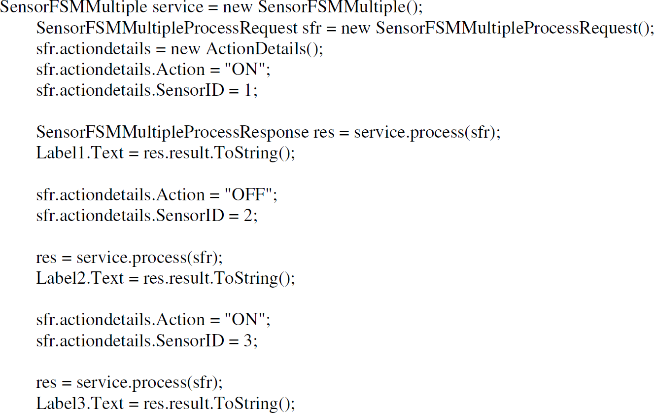
ASP.Net in C# client code.

4. Cluster Identification Using Decomposition Based on Information Transfer

Decomposition is a process of “breaking up into constituent elements.” Decompositions of systems provide a much simpler body of constituents that can best represent a given complex system. In systems science, decomposition consists of finding an optimal partition of a system in terms of its subsystems. Optimality of decomposition is evaluated by means of some adopted criteria such as a lower entropic (more information or higher negative-entropy) measure. The implication is that a “measure of complexity” of a system can be related to the entropy H(S) and information transfer T(S) functions for a system S = {X₁, X₂,…,X_n} with n ordered components X₁, X₂,…,X_n. S is not necessarily a vector with coordinates X₁, X₂,…,X_n, but represents a system with ordered components in the sense that, unless stated otherwise, all permutations of {X₁, X₂,…,X_n} stand for distinct systems. Thus, since complexity is related to information (actually, it is lack of information), the following non-negative magnitude, which is in fact a measure of information, $\sum_{i = 1}^{n} H (X_{i})$ is used to measure lack of complexity of a system when n individuals (components) are taken one by one and their inherent potentials (measured in terms of entropy) are added up. The underlying assumption for such a measure is that individuals act independently of each other not to exhibit a coherent body. Similarly, H(X₁, X₂,…,X_n) = H (S) is also a measure of information (lack of complexity) when interactive behavior of n components is taken into account, i.e., when individuals form a coherent body of a system.

T (S, P) = \sum_{i = 1}^{n} H (X_{i}) - H (X_{1}, X_{2}, \dots, X_{n})

(2)

The transfer function T(X) will now be designated by T(S, P) and will be defined in terms of the components of S. Equation (2) is a non-negative measure of change in information between a system composed of a random collection of n independent individuals and a system composed of an integrated body of these n individuals. This implies in a way that the transfer function can indicate useable information that exists in components for the system or vice versa. The larger the magnitude is, the more remote the system S will be from the chaotic case of n components being unable to form a system. The symbol P, or expressed precisely as P{X₁, X₂,…,X_n}, represents a partition of S. The notation T(S,P) hence emphasizes that information transformation depends on the given system S as well as the specific partition P of S under consideration. Roughly, “the contribution of P to T(S, P)” corresponds to the sum $\sum_{i = 1}^{n} H (X_{i})$ on the right-hand side of Equation (2) and “that of the S-part” is yielded by the term H(X₁, X₂,…,X_n) on the same side of the equation. Since we are now dealing with a system rather than the vector X, we can bring the system symbol S into Equation (1) to have the notation in Equation (2). By a partition P{S₁, S₂,…, S_q} of S, we mean a collection of disjoint subsets S₁, S₂,…, S_q, (q ≤ n), of S that exhaust S, that is, $S = ⋃_{i = 1}^{q} S_{i}$ . Therefore, the simplest partition is P{X₁, X₂,…,X_n} where q = n with S_i = {X_i} and is called an element partition. A trivial partition is P{S}, i.e., P{S} = S with q = 1. Corresponding to 1 < q < n, on the other hand, there are numerous partitions, the well known of which is dichotomous partition P{S₁, S₂}. With partition notation P{S₁, S₂,…, S_q}, information transfer function becomes Equation (3) below where H(S₁,S₂,…,S_q) is equal to H(X₁, X₂,…,X_n), since $⋃_{i = 1}^{q} S_{i} = S = {X_{1}, X_{2}, \dots, X_{n}}$ and H(S₁), H(S₂), …, H(S_q) are the corresponding entropies of the individual elements of the partition.

T (S, P) = T (S_{1}, S_{2}, \dots, S_{q}, P) = \sum_{i = 1}^{q} H (S_{i}) - H (S_{1}, S_{2}, \dots, S_{q})

(3)

When a dichotomous partition such as P{S₁, S₂} and their transmission is involved then, to emphasize the interaction between these two sets, the function T is sometimes indexed by the subscript B as in Equation (4).

T_{B} (S_{1}, S_{2}, P) = H (S_{1}) + H (S_{2}) - H (S_{1}, S_{2}) = T (S_{1}, S_{2}, P)

(4)

Similarly, to emphasize interaction within the system S = {X₁, X₂,…,X_n} with an element partition P, the magnitude T(S, P) can also be tagged as T_W(S, P), where the subscript W stands for the interaction within the system S itself. Since a coherent system can only be composed of a series system, a parallel system, or a mixture of both [20], the probability corresponding to the partition can range from the probability indicated in Equation (5) to the probability indicated in Equation (6).

P (S_{1}, S_{2}) = P (S_{1}) \times P (S_{2})

(5)

P (S_{1}, S_{2}) = m i n {P (S_{1}), P (S_{2})

(6)

The corresponding entropy of Equation (5) is H(S₁, S₂) = H(S₁) + H(S₂) and the entropy of Equation (6) is given in H(S₁, S₂) = min{H(S₁), H(S₂)}. We have thus a maximum value for T(S₁,S₂,P) that is obtained when H(S₁, S₂) = min{H(S₁), H(S₂)} and the minimum value of T_B(S₁,S₂,P) is reached when H(S₁,S₂) = H(S₁) + H(S₂), in which case T_B(S₁,S₂,P) = 0. The minimum value of the transfer function indicates that S1 and S2 are independent in statistical terms. If we let T^U_B (S₁:S₂) stand for the maximal value of T_B(S₁,S₂,P), we can obtain Equation (7).

0 \leq T_{12} = \frac{T_{B} (S_{1}, S_{2}, P)}{{T^{U}}_{B} (S_{1}, S_{2})} \leq 1

(7)

Therefore, for all systems partitioned as S₁ and S₂ and having joint distributions with fixed marginal distributions for S₁ and S₂ (systems with the given marginal distributions of S₁ and S₂), as the underlying sub-systems S₁ and S₂ become more integrated to form a whole system T₁₂ will approach to one. T₁₂ will approach to zero as S₁ and S₂ become disintegrated to form separate systems. T₁₂ is actually some version of the absolute value of the usual correlation coefficient when S₁ and S₂ are singletons like S = {X₁} and S₂ = {X₂}. Hence, T₁₂ = 0 means non-relatedness of subsets S₁ and S₂, and T₁₂ = 1 implies that S₁ and S₂ are completely dependent on each other. This latter aspect of transfer functions are emphasized in Conant [15, 16]. For comparison of the complexities of pairs of subsystems, on the other hand, Conant introduces an additional instrumental index called “interaction measure” and is defined as Equation (8).

Q_{S_{i}} (S_{j}) = T_{S_{i}} (S_{j}) - (T (S_{j}, P)) i \neq j = 1, 2 \dots q

(8)

Equation (8) is useful in detecting a change in the complexity of S_j when it is integrated into the subsystem S_i, so that the interdependence among the components of S_j are evaluated against their joint conditional interdependence given the integration of the elements of S_i. T(S_j, P) in Equation (8) denotes the conditional transmission over S_j = {X_j1, X_j2…X_jr} given the interrelatedness of the elements of S_i and is defined as Equation (9) where H_Si(S_j) = H(S_i, S_j) − H(S_j).

T_{S_{i}} (S_{j}) = \sum_{i = j_{1}}^{j_{r}} H_{S_{i}} (X_{i}) - H_{S_{i}} (X_{j_{1}}, X_{j_{2}}, \dots, X_{j_{r}})

(9)

Unlike the transfer functions T(.)'s which are always positive, the interaction measure Q(.) in Equation (8) can be negative (i.e., the sets S_i and S_j interact negatively), positive (i.e., S_i and S_j have positive interaction between them) or zero (i.e., S_i and S_j are stochastically independent). Usefulness of the information transfer functions in Equation (2) and Equation (3) for applications of systems is two-fold. Obviously, when we have no usable information, or conversely when we have full information, on both S and P, the function T(S, P) ceases to be of some use. Its use becomes accentuated when we have partial information on S and/or P. In fact, we may be in a position to obtain a system with some given subsystems or to derive some subsystems from a given system. The former problem is composition (integration) and the latter is decomposition. In the composition issue, P is known but we have no knowledge about S. In the decomposition problem, we have information on S but none about P. Information on P and/or S means knowledge about the distributions involved as well. The concept information used here either is in the information theoretic sense, for example, the information transfer function, or is in the daily usage sense, that is “knowledge.” Thus, for obtaining the solution of the integration problem, the information transfer function is maximized over all possible systems S = {S|S ∊ S} which yield the given common partition P. In other words, H(S) = H(S₁,S₂,…,S_q) or H(X₁, X₂,…,X_n) is minimized. Conversely, a solution for decomposition (partition P) is obtained by minimizing the transfer function over all possible partitions of the given system S. 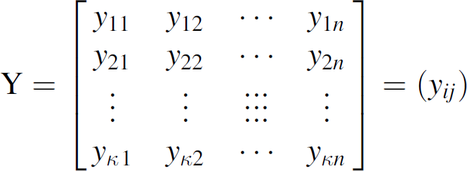In other words, $\sum_{i = 1}^{q} H (S_{i})$ or $\sum_{i = 1}^{n} H (X_{i})$ is minimized. All foregoing discussions and indices are undoubtedly relevant for the case where we know the distributions. When such information is unavailable, as consistent estimates, we can use empirical distributions. Collection of observations for the purpose is however costly and hard to obtain. This is true for empirical assessment of joint distributions, when we are especially interested to obtain estimates of multivariate distributions for large sets of components. The following illustrate the initial stages where observations on element partition and pair-wise partition of the system are available.

4.1. Illustration 1

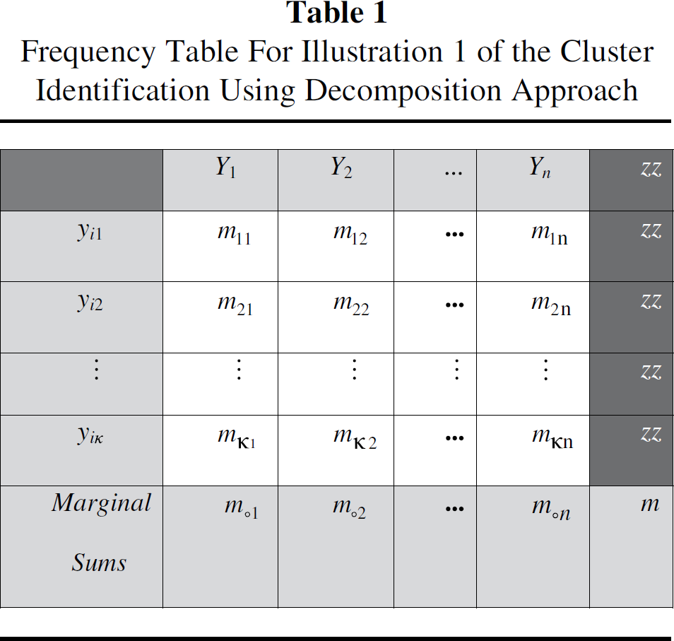
A simple empirical case corresponds to availability of observations on each individual component. Let S = {Y₁, Y₂,…,Y_n} hence be a system with n ordered components and with the given matrix Y given in Equation (10) of discreet observations where y_ij denotes the i^th functional value (i = 1, 2,…, k) taken up by the j^th component of the system S = {Y₁,Y₂,…,Y_n}. Assume further that these values are observed with the frequencies as in Table 1.

Y = [\begin{matrix} y_{11} & y_{12} & \dots & y_{1 n} \\ y_{21} & y_{22} & \dots & y_{2 n} \\ ⋮ & ⋮ & \dots_{\dots}^{\dots} & ⋮ \\ y_{κ 1} & y_{κ 2} & \dots & y_{κ n}) \end{matrix}] = (y_{i j}

(10)

By definition, the magnitudes m_io and m in Table 1 are

\sum_{j = 1}^{κ} m_{i j} = m_{i \circ}

and

\sum_{i = 1}^{n} m_{i \circ} = m

. Clearly, these observations are sufficient to obtain estimates for marginal distributions of the individual components Y₁, Y₂,…,Y_n. Another easy to follow real life example for this case corresponds to the frequency of long distance phone calls m_ij placed at a certain geographical location Y_i at some given time unit y_ij. Consider the element partition P{S₁,S₂,…,S_n} of S where S_i = {Y_i} for each component Y_i. Thus, the marginal probability of each component S_i = {Y_i} is P(S_i) = π_i which can be consistently estimated by

{\hat{π}}_{i} = \frac{m_{i \circ}}{m}

. For each component Y_i, the probability of the event {Y_i = y_ij} is represented by P(Y_i = y_ij|S_i) = π_j|i and the latter will similarly be estimated by

{\hat{π}}_{j | i} = \frac{m_{i j}}{m_{i \circ}}

. However, after observing the system S, the probability for the same event {Y_i = y_ij} becomes P(Y_i = y_ij|S) = π_ij and is estimated with

{\hat{π}}_{i j} = \frac{m_{i j}}{m}

. Accordingly, Equation (11) provides the estimates for the entropies of individual components and Equation (12) provides the estimate for the system entropy.

Table 1

Frequency Table For Illustration 1 of the Cluster Identification Using Decomposition Approach

	Y ₁	Y ₂	…	Y _n	zz
yi1	m ₁₁	m ₁₂	…	m _1n	zz
y _i2	m ₂₁	m ₂₂	…	m _2n	zz
⋮	⋮	⋮	⋮	⋮	zz
y _iκ	m _κ 1	m _κ2	…	m _κn	zz
Marginal Sums	m _°1	m _°2	…	m _°n	m

H ({\hat{S}}_{i}) = - \sum_{j = 1}^{κ} \frac{m_{i j}}{m_{i \circ}} log (\frac{m_{i j}}{m_{i \circ}}), i = 1, 2, \dots, n

(11)

H ({\hat{S}}_{1}, S_{2}, \dots, S_{n}) = - \sum_{j = 1}^{n} \sum_{i = 1}^{κ} \frac{m_{i j}}{m} ((log \frac{m_{i j}}{m}))

(12)

The estimated information transfer will be

\begin{aligned} T r (\hat{S}, P) & = \sum_{i = 1}^{n} H ({\hat{S}}_{i}) - H (S_{1}, {\hat{S}}_{2}, \dots, S_{n}) \\ = - \sum_{j = 1}^{κ} \frac{m_{i j}}{m_{i \circ}} log (\frac{m_{i j}}{m_{i \circ}}) + \sum_{j = 1}^{n} \sum_{i = 1}^{κ} \frac{m_{i j}}{m} ((l o g \frac{m_{i j}}{m})) \end{aligned}

(13)

A vanishing value of this non-negative real number in Equation (13) provides some evidence that the partition P{S₁, S₂,…,S_n} conforms well with the given system S, so that the degree of its divergence from zero is a clue that there is still some unused information in P{S₁, S₂,…,S_n} for S or vice versa Accordingly, when $T r (\hat{S}, P) = 0$ , observations suggests that the system cannot be decomposed further than the element decomposition P{S₁,S₂,…,S_n}. A non-vanishing value of the empirical information transfer function $T r (\hat{S}, P)$ thus suggests that it is worthwhile to seek decompositions other than P{S₁,S₂,…,S_n}. We can clearly partition S in some other way such as P{S₁, S₂,…,S_q} where 1 < q < n. The foregoing analysis can be repeated using (14) for this case to check whether P{S₁, S₂,…,S_q} has some information for S. In that case, the system entropy estimate $H (S_{1}, {\hat{S}}_{2}, \dots, S_{n})$ will stay put, but estimates of entropies $H ({\hat{S}}_{ℓ})$ of individual subsets S_ℓ will change. The given observations in the frequency Table 1 are clearly not sufficient to obtain a conclusion beyond the result obtained above. For further conclusion, we need more sophisticated observations and experiments. Hence, we introduce next, the second Illustration.

4.2. Illustration 2

The second illustration relates to a case where empirical data for pairs of components are available. Obviously, this case is more general in the sense that the availability of empirical observations (frequencies) on pairs of random variables implies also the availability of observations on individual variables as well. Assume again, for simplicity of exposition, that the random components Y₁, Y₂,…, Y_n−1 and Y_n are discreet in nature and the number of functional values taken by each Y_i is r_i, (i = 1,2,…,n) with these values ranging over the whole numbers y_i1, y_i2,…y_ir_i. For notational convenience and without loss of generality, we can assume that r_i = r for all i = 1,2,…,n. As such, in accordance with a certain pattern, the joint event {Y_i = y_ih, Yj = y_jk}, i ≠ j, takes values in the discrete (r(n−1)) × (r(n − 1)) matrix layout set up as in Table 2. This layout is now our observational system T, which is a proper subset of S × S.

Table 2
Pair-Wise Observations for Illustration 2 of the Cluster Identification Using Decomposition Approach

Y₁ Y₂ … Y_i … Y_j … Y_n

Y₁

Y₂

⋮

Y_i

⋮

Y_j

⋮

Y_n

m

Since we are interested in cross pairs of variables like Y_i and Y_j with i ≠ j, the diagonal block cells (shaded in darker gray) of Table 2 are irrelevant and we therefore have (n−1) rows and (n−1) columns of interest. Hence, off-diagonal cells become a center of interest. Each off-diagonal block cell in Table 2 is composed of an (r × r) matrix of observations on the bi-variable event such as {Y_i = y_ih, Y_j = y_jk}, i ≠ j = 1,2,…,n and h,k = 1,2,…,r. When the two events {Y_i = y_ih Y_j = y_jk} and {Y_j = y_jk,Y_i = y_ih} are identical, i.e., when they are symmetrical, then only the upper or lower off-diagonal part of Table 2 can be used. For convenience of visualization, the unused part (for instance, the lower part) is shaded in light gray in Table 2. In this latter case, the upper off-diagonal block cells become the system Tof observations to be considered. The bottom row and the last column shaded in blue are empty and the cell in the south east corner contains one single element marked m representing total number of observations. To aid exposition, the block cell corresponding to the observational frequencies on the i^th and j^th variables (shaded in orange color in Table 2) is reproduced in Table 3 with the same color. For the specific pair of Y_i and Y_j, the symbol m_i(h)j(k) of Table 3 stands for the frequency with which the bi-variable event {Y_i = y_ih Y_j = y_jk} is observed empirically. The last column and the bottom row of Table 3 present marginal frequencies involved. For observations on {Y_i = y_is} corresponding to a certain s=1,2,…,r, we have Equation (14) and similarly, for a certain t =1,2,…,r, we have Equation (15).

Table 3

Frequencies of {Y_i = Y_ih, Y_j = Y_jk} in Table 2 for The Highlighted Pair of I and J

m _i(1)j(1)	m _i(1)j(2)	…	m _i(1)j(r)	m _i(1)j
m _i(2)j(1)	m _i(2)j(2)	…	m _i(2)j(r)	m _i(2)j
⋮	⋮	⋮	⋮	⋮
m _i(r)j(1)	m _i(r)j(2)	…	m _i(r)j(r)	m _i(r)j
m _ij(1)	m _{i j(2)}	…	m _ij(r)	m _{i j}

m_{i (s) j} = \sum_{k = 1}^{r} m_{i (s) j (k)}, i \neq j

(14)

m_{i j (t)} = \sum_{h = 1}^{r} m_{i (h) j (t)}, i \neq j

(15)

Thus, we can obtain Equation (16) where $m = \sum_{i = 1} \sum_{i < j} m_{i j}$ .

m_{i j} = \sum_{s = 1}^{r} m_{i (s) j} = \sum_{t = 1}^{r} m_{i j (t)}

(16)

As shown in Table 2, m is located in the southeast cell of the table. The $q = \frac{n (n - 1)}{2}$ upper off-diagonal block cells of Table 2 can now be labeled as T₁, T₂,…,T_q. Obviously, P{T₁,T₂, …,T_q} is a proper partition of T. Labeling starts from the top leftmost cell of the table, it then goes to the leftmost off-diagonal block cell of the second row and so on as in the lexicographical ordering: T₁ for {Y₁,Y₂}, T₂ for {Y₁,Y₃},…, T_q for {Y_n−1,Y_n}. For each partition ℓ= (i,j), i < j estimates of the marginal probabilities P(Y_i = y_ih Y_j = y_jk) = π_i(h)j(k), j > i = 1,2,…,n and h,k = 1,2,…,n, is given by Equation (17). Furthermore, for the whole system the same estimate becomes Equation (18) so that, as before, we obtain Equations (19) and (20).

\hat{π} i (h) j (k) | ℓ = \frac{m_{i (h) j (k)}}{m_{i j}}

(17)

\hat{π} i (h) j (k) = \frac{m_{i (h) j (k)}}{m}

(18)

H ({\hat{T}}_{ℓ}) = - \sum_{h = 1}^{r} \sum_{k = 1}^{r} \frac{m_{i (h) j (k)}}{m_{i j}} l o g (\frac{m_{i (h) j (k)}}{m_{i j}})

(19)

H (T_{1}, {\hat{T}}_{2}, \dots, T_{1}) = - \sum_{i = 1}^{n} \sum_{i < j}^{n} \sum_{h = 1}^{r} \sum_{k = 1}^{r} \frac{m_{i (h) j (k)}}{m} l o g (\frac{m_{i (h) j (k)}}{m})

(20)

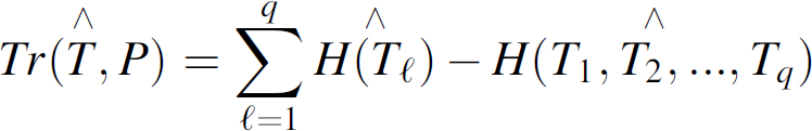
Thus, the estimated transfer function in Equation (21) will have small values close to zero when pair-wise partition is enough for decomposition, whereas its higher values will produce evidence that there is some further information to be utilized in T for further partition P{T₁, T₂,…,T_r}, q ≠ r.

T r (\hat{T}, P) = \sum_{ℓ = 1}^{q} H ({\hat{T}}_{ℓ}) - H (T_{1}, {\hat{T}}_{2}, \dots, T_{q})

(21)

5. Simulation of Sensor Network Orchestration Using Agents

SOMA use two classes of intelligent agents to aid in orchestration: Field-Agents and Process-Agents. Field-Agents monitor and provide internal status and information about sensors, monitors battery levels and exceptional conditions in the system. Process-Agents monitor the cluster status at any time and dynamically orchestrate the cluster to reduce the detection signature, determine the strengths of the communication activity between the groups of clusters, and group clusters or destroy them to reduce communication between sensors and prevent detection.

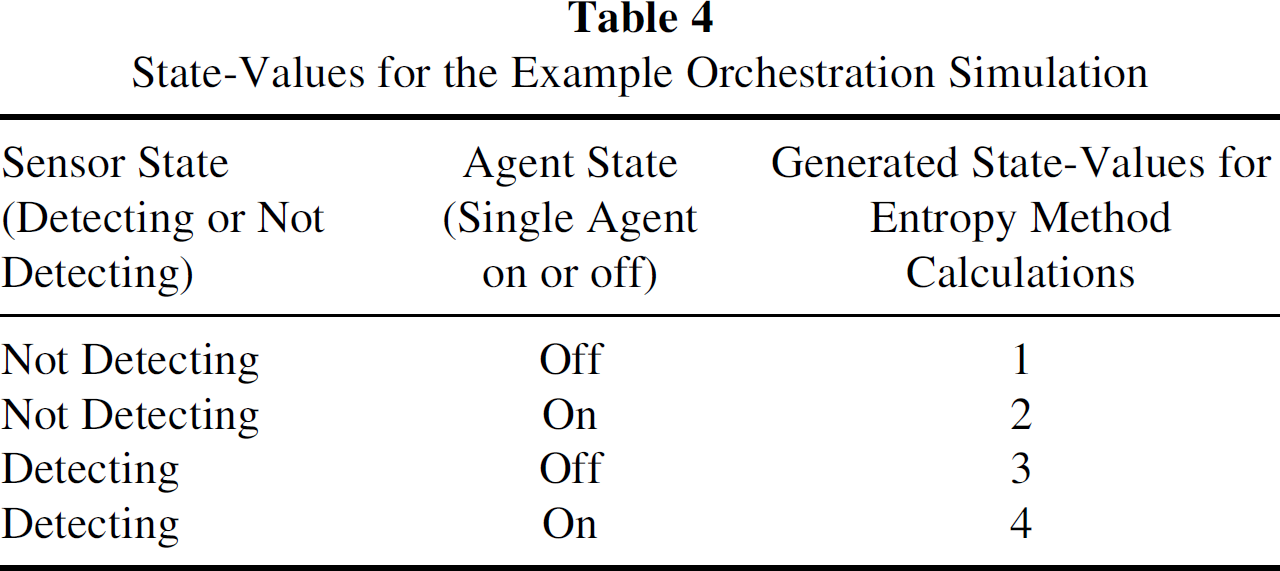
In the simulation, we have assumed that each sensor has one Field-Agent. The Process-Agent collects data from the Field-Agents in the sensors. The states of operations (state-values) at an instance of time of a sensor were indicated to be one, two, three, or four. The state-values are based on two variables. One is the state of the Field-Agent associated with the sensor, and the second is the detection state of the sensor. Currently, we have implemented the decomposition method in Java and Matlab, and these two implementations are used to verify and validate the calculations of each other. The data in these calculations are simulated by taking into account realistic situations.

4.3. Pre-Orchestration Phase

Table 4 shows the state-values based on a simulation of the expected target track. Figure 2 shows the plot of the normalized transmissions calculated for the data set of this phase. Based on Table 5, sensors with transmission values higher than the set threshold value (we assumed it as 60% of the maximum transmission value) were identified as “busy sensors.” The maximum transmission value of Table 4 data set was calculated to be 1.3480 and the threshold value to be 0.8088. From the above transmissions (25 × 25 array of transmission values), the following sensors indexes were determined to have a transmission value higher than the set threshold value: 1, 2, 3, 6, 7, 8, 26, 27, 28, 31, 32, 33, 51, 52, 53, 56, 57, 58, 79, 80, 89, 90, 104, 105, 114, 115, 126, 127, 128, 131, 132, 133, 151, 152, 153, 156, 157, 158, 176, 177, 178, 181, 182, 183, 326, 327, 328, 329, 330, 331, 332, 333, 339, 340, 351, 352, 353, 354, 355, 356, 357, 358, 364, 365, 469, 514, 515, 539, 540, 564, 565, 589, 590, 614, and 615.

Table 4
State-Values for the Example Orchestration Simulation

Sensor State (Detecting or Not Detecting) Agent State (Single Agent on or off) Generated State-Values for Entropy Method Calculations

Not Detecting Off 1

Not Detecting On 2

Detecting Off 3

Detecting On 4

Sensor State (Detecting or Not Detecting)	Agent State (Single Agent on or off)	Generated State-Values for Entropy Method Calculations
Not Detecting	Off	1
Not Detecting	On	2
Detecting	Off	3
Detecting	On	4

Figure 2

Transmissions plot for the 1st time phase of the single-agent approach.

The analysis of the data revealed that sensors numbered 1, 2, 3, 4, 5, 6, 7, 14, 15, 19, 21, 22, 23, 24, and 25 were involved in majority of the transmissions in the network. Of these, most of the transmissions were taking place between the sensors numbered 1, 2, 3, 4, 5, and 6. Additionally, sensors numbered 14 and 15 had high transmissions between them.

Table 5

Simulated Data Set of the Example Orchestration Simulation

4.4. Orchestration Phase

The Process Agents is used to turn-off the Field-Agents in the above busy sensors and orchestrated (distributed the load) to other sensors in their proximity, which had their Field-Agents state as OFF. The reconfigured transmissions after orchestration were calculated and the plot in Fig. 3 shows the transmissions plot for a data set collected from these sensors. Comparing Figs. 2 and 3 (plotted with intensity of communications in the Y-axis), we can see that the orchestration method in SOMA has successfully reduced the intensity of transmission.

Figure 3

Transmissions plot after agent-switching in the 1st phase of the one-agent approach.

By carefully applying the orchestration method in the example simulations, we demonstrated that at least two of the Micro-DADS related challenges can be addressed using SOMA. These two challeges are to improve the energy efficiency of the sensors, and reduce their probability of detection. In this paper, we estimate that if the intensity of communication of a sensor cluster is above a certain threshold level, then there is greater probability of detection and the sensors are less energy efficient. Therefore, by reducing the intensity of communication in a cluster by “switching” the activities of busy sensors to nearby sensors through orchestration, we have reduced the probability of detection and increased the efficiency of the sensors.

6. Conclusion and Future Work

The article outlines some of the challenges the Navy faces because of its shift to a distributed architecture in the Micro-DADS program from a central architecture in the DADS program. Primary among those challenges is the ability to conserve energy and prevent detection. Adopting the orchestration model of Web Services and employing a formal decomposition technique based on entropic analysis, we introduced a Service-based Orchestration Model using Agents (SOMA) for efficient and effective control and coordination of self-configuring sensor systems. The decomposition technique used in SOMA is free from restrictions of structural modeling and does not depend on the type of distribution of the random variables involved. It does not require either any restriction on the type of interaction of variables such as their uncorrelatedness or independence. The operational steps in SOMA are shown using simulations. The example simulations demonstrate the potential of SOMA addressing two of the important problems of Micro-DADS, namely

battery life maximization, and

minimization of detection probability.

References

Raysin

Alspaugh

Ivancic

, “System analysis of Deployable Autonomous Distributed System (DADS) network communication study,” CDRIL, Item A001, September 1998.

“Future DADS and USW Concept Briefing.” VA: Office of Naval Research Arlington, 2001.

Tubaishat

Madria

, “Sensor networks: an overview,” Potentials, IEEE vol. 22, pp. 20–23,2003.

Iyengar

, “Computational aspects of distributed sensor networks,” in Proceedings of the International Symposium on Parallel Architectures, Algorithm and Networks, Makati City, Metro Manila, Philippines, 2002, May 22–24.

Davis

Hasegawa

Kadowaki

Obana

, “Self-organization of activity in wireless sensor networks,” International Journal of Distributed Sensor Networks vol. 1, pp. 245–252,2005.

Guru

S. M.

Hsu

Halgamuge

Fernando

, “An extended growing self-organizing map for selection of clusters in sensor networks,” International Journal of Distributed Sensor Networks vol. 1, pp. 227–243,2005.

Cerpa

Estrin

, “ASCENT: adaptive self-configuring sensor networks topologies,” Mobile Computing, IEEE Transactions on vol. 3, pp. 272–285,2004.

Iyengar

S. S.

Brooks

R. R.

, Distributed Sensor Networks. Boca Raton, FL: Chapman & Hall/CRC, 2004.

Sadasivam

R. S.

Goli

Krishnan

Mamuwallah

Tanik

M. M.

, “Dynamic reconfiguration of field-agents to process-agents in distributed systems,” in Proceedings of the IDPT 2004, Turkey, 2004, June 28- July 2.

10.

Goli

, “A dynamic entropy-based model for reconfiguring the communications in hierarchical distributed sensor systems,” M. S. thesis, Electrical and Computer Engineering, University of Alabama at Birmingham, Birmingham, 2004.

11.

Krishnan

, “Dynamic management of sensor fields using entropy,” M. S. thesis, Electrical and Computer Engineering, University of Alabama at Birmingham, Birmingham, 2004.

12.

Thompson

S. C.

, “Process of selecting message trunk configurations for an overlay packet voice tandem,” M. S. thesis, Electrical and Computer Engineering, University of Alabama at Birmingham, Birmingham, 2004.

13.

Kathiru

R. R.

, “Dynamic mobile agent routing algorithm in a distributed sensor network” M. S. thesis, Electrical and Computer Engineering, University of Alabama at Birmingham, Birmingham, 2005.

14.

Juric

M. B.

Mathew

Sarang

, Business Process Execution Language for Web Services: BPEL and BPEL4WS, Packt Publishing, 2004, pp. 270.

15.

Conant

R. C.

, “Information transfer in complex system: with applications to regulations,” Ph.D. dissertation, Graduate School, University of Illinois, 1968.

16.

Conant

R. C.

, “Detecting subsystems of a complex system,” IEEE Transactions on Systems, Science, and Cybernetics, pp. 550–553, 1972.

17.

Simon

H. A.

, The Sciences of the Artificial. Cambridge, Massachusetts: MIT Press, 1969.

18.

Tuncer

Tanik

M. M.

Allison

, “An overview of statistical techniques applied to complex systems,” Department of Computer and Electrical Engineering, University of Alabama at Birmingham, Birmingham, Al 2006–02, 2006.

19.

Papoulis

Pillai

S. U.

, Probability, Random Variables and Stochastic Processes, 4 ed: McGraw-Hill Science/Engineering/Math, 2001.

20.

Barlow

R. E.

Prochan

, Statistical Theory of Reliability and Life Testing Probability Models: Holt, Rinehart and Winston, Inc., 1975.

A Service-Based Entropic Model for Sensors Orchestration