Sage Journals: Discover world-class research

Abstract

Sensor networks are typically wireless networks composed of resource-constrained battery powered devices. In this paper, we present a criterion for determining whether or not a surveillance sensor network is viable. We use this criterion to compare methods for extending the effective lifetime of the sensor network. The life extension methods we consider are local adaptations that reduce the energy drain on individual nodes. They are communications range management, node repositioning, and data agreement. Simulations of a surveillance scenario quantify the utility of these methods. Our results indicate that data agreement provides the most improvement in network longevity, and communications range management is also useful. Repositioning nodes to reduce the power needed for communications is dependent on the amount of attenuation experienced by the node's communications signal and the volume of traffic between nodes. When these factors are considered, node repositioning is an effective strategy for network life extension. Synergies between the energy conservation approaches are also explored.

Keywords

Sensor Network Power Conservation Distributed Adaptation Surveillance

1. Introduction

This paper considers the methods for extending the effective lifetime of wireless sensor networks used for surveillance applications.

The first question we address is “when is a surveillance network viable?” As explained in section 2, network viability can be determined using the consequences of the ad hoc network topology model first given in [14] and extended in [6]. This provides a straightforward technique for determining whether or not a surveillance network can adequately perform its task.

In our analysis, we will assume that all sensor nodes have the same configuration, namely:

There is a generic sensor for target detection.

Computations can be performed locally.

Wireless communication is used for coordination and reporting results.

Global Positioning System (GPS) provides a common clock and accurate localization. (This requirement is not strict. As long as the position errors are not correlated, and clock skew remains within reasonable bounds, and the results given in this article will hold.)

Nodes are mobile. In this case, we consider nodes with wheels that can move under their own volition.

In our analysis, target detection is triggered by the Closest Point of Approach (CPA) events [3]. The sensors are imperfect. We allow for non-trivial false negative (type 1) and false positive (type 2) error rates. The sensing model is given in section 4.

Section 3 reviews relevant literature on sensor node power issues. We assume nodes fail when their battery power is exhausted and use a crash-fail model (i.e., when a node fails it ceases to perform all functions permanently). Nodes can use their last energy to inform neighbors of their imminent failure. We do not consider node failures for other reasons. Sensing errors are not considered failures.

The life extension techniques we consider are evaluated using a simulation tool presented in section 4. The simulation implements the local life extension behaviors presented in section 5, along with bookkeeping to track node power use. Node behaviors are reactions to target movement in the region monitored by the network. In the simulation, target trajectories are spline curves passing through three random points. In section 5 we discuss the power optimizations:

Dynamic modification of wireless transmission range.

Node movement to reduce communications range or compensate for node failure.

Local aggregation of sensor readings to reduce network traffic due to type 1 and type 2 sensing errors.

Section 6 considers combinations of these approaches.

The main contributions of this paper to the literature are:

Presenting a network viability criterion for surveillance applications.

Providing simulation results comparing power conservation approaches for practical applications.

Illustrating how node mobility can be used to extend network lifetime, contradicting the disappointing results for node repositioning given in [33].

Exploring the effect of combining multiple node power optimizations.

The paper is structured as follows. Section 2 discusses network viability. Sensor network power consumption is reviewed in Section 3. Section 4 explains the simulation used to find the expected sensor network lifetime. In Section 5, we describe two methods for reducing power consumption and compare them using network simulations. Section 6 looks at node relocation issues in detail. Section 7 looks at second order effects of integrating power optimizations. In Section 8 we discuss other network life extension approaches. We conclude the paper with a discussion of our results and future extensions in Section 9.

2. Network Vialbility Criterion

Consider a surveillance network charged with reporting when a member of a class of objects (targets) traverses a given surveillance domain (terrain). Reports are sent to a user community that we assume, for the sake of discussion, is external to the terrain. The community is alerted to a detection event by a detection packet reaching the network periphery. The surveillance network will be viable as long as it assures that:

(i)
an object traversing the terrain is detected (with acceptable error rates), and
(ii)
the user community is alerted.

These properties must exist almost surely (i.e., with a probability of 1 [2]). Our criterion is a tautology: the network is viable as long as it can continue to perform its mission.

To date, the implications of this tautology have been overlooked. For example, the following methods of determining network viability do not fit the criterion:
Network connectivity – If full network connectivity is needed, the sensor network is a giant serial system. Network availability will fall exponentially with the number of sensor nodes (n), and thus large networks will have an unacceptable mean time to failure. For networks with any redundancy, some nodes can be isolated from the network without compromising its application.

Sensing coverage – refers to placing nodes so that sensor detection regions have little overlap, but the system monitors the entire terrain. Since sensing ranges and coverage regions are unpredictable, problems with this “cookie cutter” approach are well known [27]. The problems are often due to environmental influence [24]. Real-world approaches consider distributed surveillance as a tracking problem using sensors with finite space and time sampling rates [4, 5]. Coverage approaches ignore sensor errors, background noise, and occlusion. In addition, coverage analysis creates a serial system, which fails when any component fails. Once again, we have a serial system where dependability falls exponentially with network size.

2.1. Network Connectivity Ignores Sensing Issues. Sensing Coverage Ignores Wireless Communications Issues

We propose a network viability criterion that is a direct consequence of the network model in [14] where nodes with a fixed communications range are placed at random in the terrain. Simulations show that ad hoc networks with range limited communications exhibit phase change phenomena like those found in the random graph [2] and percolation [23] theories. The random graph theory is a branch of graph theory that assigns probability distributions to the existence of edges between vertices. Percolation theory, a branch of physics, studies fluid flows in random media. Random media are modeled as tessellations of a terrain with probability distributions for the existence of edges between neighboring vertices. Reference [6] discusses their common basis.

In these models, network behavior has two phases. In the first phase, the probability of connection between nodes is small and the network has a large number of isolated components. As the connection probability grows, the expected size of the largest component grows logarithmically. In the second phase, the network is dominated by a unique giant component that contains most of the system nodes. There are still isolated holes in the network. The size of the largest hole shrinks logarithmically as the connection probability increases. The transition between these two phases is extremely steep. For random graphs, the curve of the maximum component size versus the edge probability takes the form $e^{- e^{- c}}$ . In percolation theory, the inflection point of this curve is referred to as the percolation threshold.

The percolation theory has established these properties for systems with a giant component [23]:

For systems above the percolation threshold, a path exists that connects the external boundaries of the terrain.

At the percolation threshold, property 1 is self-similar over scales (i.e., it holds over samples of the terrain of any size). Readers unfamiliar with self-similarity are encouraged to refer to [23].

Consider sensor networks with nodes either randomly placed [14] in a regular tessellation [23] or a weighted combination of the two. Sensor nodes are vertices in a random graph structure. Edges between vertices represent either an active communications link, or detection of a target passing between nodes. In practice, the edge probability distribution is the minimum of the two likelihoods.

Above the phase change (percolation threshold) a single giant component connects most of the sensor nodes (O(n)) [23]. It has at least one path connecting all the terrain's external boundaries (property 1). This property is true for subsets of the system across scales (property 2). Thus, for a sensor network with a giant component, targets traversing the network will be detected by at least one node that is able to report the detection to the user community. Therefore, the network fulfills our viability criterion.

Note the subtle differences between this and the coverage and connectivity criteria. Coverage is not guaranteed, because small sensing gaps may exist in the terrain surveyed. But these gaps are of limited size and surrounded by regions that are covered, any target will be detected before or after it enters a gap. Similarly connectivity is not guaranteed, since isolated nodes exist that are not connected to the network as a whole. But paths will exist from other nodes to the user community (in this case the periphery), so the loss of these isolated nodes does not stop the network from functioning correctly. Above the percolation threshold, the system is dense enough that the loss of these isolated nodes does not keep the network from performing its task. Compare this to the criteria used in sensing coverage and network connectivity studies, where the whole network is incapacitated as soon as any single node is disabled.

In our approach the network is viable as long as it contains a giant component. In our simulation, we infer the loss of the giant component from the loss of property 1. When there is no path between the terrain's external boundaries, the giant component is fractured. Consider the worst-case scenarios for networks with initial configurations above the percolation threshold:

A target entering the network cannot be detected and/or reported while in a hole. Since the largest hole above the percolation threshold is O(log n) [2, 23], this is the upper limit of the target's ability to avoid detection in the initial network configuration.

As nodes lose power:

(i)
maximum hole size grows logarithmically,
(ii)
the network becomes sparse, and
(iii)
the network approaches the percolation threshold.

As long as we are above the percolation threshold property 1 holds and a target has to pass through a graph edge to traverse the terrain. Once it does so, a node connected to the giant component detects the target and notifies the user community. Property 2 says that property 1 holds for regions inside the terrain up to the percolation threshold.

A fuller treatment of these issues and how to predict the percolation threshold for systems is in [6].

This concept is different from the dominating set approaches used in [31] and [32]. While those papers consider both sensor coverage and network connectivity simultaneously, they attempt to guarantee coverage over the entire surveillance region. They use massive redundancy that fields more nodes than needed at any moment. The approach we suggest allows networks to be fielded that are viable and do not contain massive redundancy; for some applications this could result in significant cost savings.

Also, in [31] and [32], the network lifetime is extended by choosing subsets of nodes to sleep and conserve energy. These subsets disrupt neither sensing coverage nor network connectivity. Note that local signal (sensor or communications) disruptions can negate the results of these approaches by causing local violations of the global policy. The criterion given here guarantees that with high probability (for very large networks this can be a probability of 1 [2]) any gaps will be enclosed by regions where surveillance is active. Disruption of the global network would require jamming signals over a large area, which would be prohibitively expensive.

Conserving power by allowing nodes to sleep is the equivalent of pre-positioning node replacements in the field, and the approaches in [31] and [32] require more coordination between nodes than our approach. These comments do not denigrate the work in [31] and [32], which is important and largely orthogonal to our work. They are meant to contrast those solutions, which concentrate on maintaining local attributes, and our solution, which is willing to sacrifice nodes and local coverage, as long as the global application continues to function.
3. Review of Sensor Network Power Consumption

We now review sensor node power consumption literature to motivate the simulation scenario and power conservation techniques. Sensor networks rely on battery power. [20] researches the use of ambient energy sources to power sensor networks and comes to the unfortunate conclusion that, although promising, this is not currently feasible. Reliance on limited, non-renewable battery energy resources means that to achieve a reasonable network lifetime, all aspects of sensor networks must be energy efficient.

Some publications state that computation power needs will decrease until negligible, and wireless communications energy will dominate the energy consumption by sensor networks [18, 1]. This logic combines Moore's law stating that feature sizes halve every 18 months with the fact that smaller feature sizes require less power. Unfortunately, this ignores important factors:

(i)
leakage energy consumption grows as feature size decreases, and
(ii)
Moore's law also states that clock rates increase at the rate feature sizes shrink. Faster clock rates require more energy. Realistic energy models for sensor networks will have to account for all aspects of node behavior.

From the power consumption analysis in [9]:
For most commercial ARM8 processor instructions, the energy required is 4.3∗10⁻⁹ joules per bit. Multiplication requires 31.9∗ 10⁻⁹ joules per bit.

Berkeley smart dust prototypes consume 0.05∗ 10⁻⁹ joules per bit for most instructions (multiplication not supported).

Radio frequency ground communications require 10⁻⁷ joules per bit for 0–50 meters, and 50∗ 10⁻⁶ joules per bit for 1–10 kilometers.

The mote and radio figures are lower bounds, based on research prototypes. Commercial products are unlikely to reach these levels of efficiency in the near future:
Per bit energy consumption for multiple instructions on commercial processors is in the range 48 (MC68328 DragonBall) to 0.84 (SA-110 StrongARM)∗ 10⁻⁹ joules per bit [7].

Communications require from 40∗ 10⁻⁶ joules (GSM cellular phone) to 1∗ 10⁻⁷ joules (Bluetooth for 10s of meters) per bit [9].

Reception energy needs for GSM are 2∗10⁻⁶ joules per bit, and 10⁻⁷ joules per bit for Bluetooth. [9].

Energy needs for communications are proportional to r^−α where r is the range. The α exponent is in the range 2 to 5. A value of 3.5 is reasonable for many applications [29]. For commercial and prototype systems, transmitting one bit for one hop is on the order 10² times more expensive than computing one instruction on one bit.

[9] and [19] claim transmission energy is the dominant drain on sensor networks when per hop communication is over 10 meters. This claim is based on applications with minimal on-board computation. Two examples in [9] only sample data, do analog-to-digital conversion, execute a filter, and transmit data. The other example does a least squares estimate of vehicle velocity from five data samples. This amounts to executing one very small matrix multiplication. For nodes with minimal to no local data processing, the communications energy consumption is certain to dominate the computation energy requirements.

Our empirical tests indicate that, for many classes of sensor network applications, computation dominates energy consumption. In [22, 15, 16] beamforming [8] and CPA based tracking approaches [3, 4, 5] are compared. The beamforming approach was found to be more accurate, while requiring 10³ times more energy. Communications energy requirements were calculated from the bluetooth energy per bit. Computation energy was measured on an AMD Athlon 4 mobile processor. The communication was responsible for less than 20% of the total energy drain. Both applications used embedded Linux. Beamforming is computation intensive, performing cross-correlation over multiple time series to estimate the signal direction of arrival. The CPA based approach requires minimal computation. This study of representative sensor network applications supports the view that power awareness must consider computation and communication.

For secure applications, both [7] and [17] show that encryption, decryption, and secure hashing are computation intensive, with a large energy overhead. [7] measures the energy drain of key initialization communications on sensor networks.
4. Simulation Environment

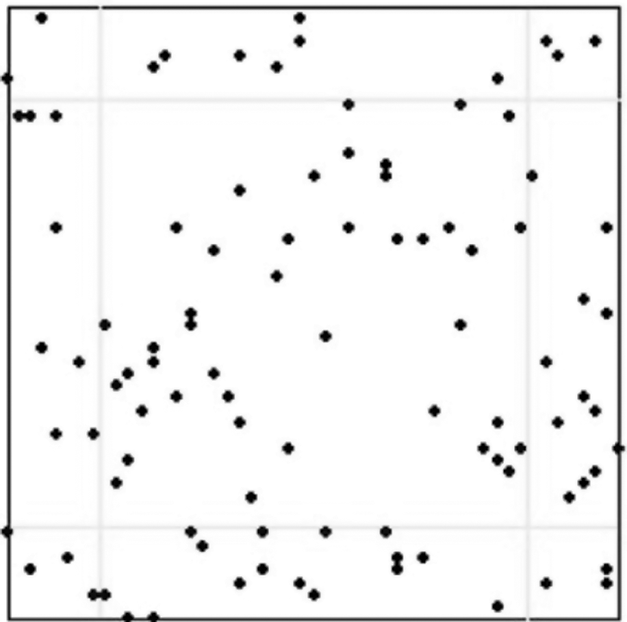
To study the effect of power conservation on network lifetime, a surveillance sensor network simulation was implemented. The network used topologies based on the model in [14]. The method in [6] was used to guarantee that initial network configurations were above the percolation threshold and had a giant component. The simulation environment resembled the field test we performed at 29 Palms Marine Base [4], where the effective sensing range was much greater than the wireless communications range. We determined whether or not the network was viable at any point in the simulation by verifying empirically that communications paths existed between all four terrain boundaries. Figure 1 shows a sample display from the simulation.

Figure 1.

Simulation snapshot. Dark points are active nodes. Dull nodes are in a low power state. Light colored nodes are dead. The star is the target position. Nodes within the circle can detect the target.

We considered a sensor network operating within a 50 m × 50 m square area. Each node was given an initial energy of 2880 J. Since lithium batteries have better energy density (2880 J/cc) and longevity than Zinc-air and Alkaline batteries we used them as our power model [20].

The simulations were started with 100 nodes and increased till 1000 in steps of 100 nodes. The decision to start the simulation with 100 nodes was taken after observing the phase change graph of the test results. Figure 2 shows where the percolation threshold is crossed and the giant component starts to form.

Figure 2.

Mean network lifetime vs the number of nodes showing a phase change where the giant component forms.

We modeled the nodes after Berkeley Motes, which require 1 pico joule per instruction computed, 100 nano joules per bit transmitted, and 4 nano joules per sensor sample [9]. The energy required for data packet reception is constant, as is the energy required for computation and sensing. This power drains at a constant rate while nodes are active. We model only the energy consumption due to packet transmission and node movement. The influence of the other drains can be factored in to our results by using a constant factor times the time t.

The detection packets broadcast by nodes were 56 bytes long as in [29]. The maximum communications range is 7.5 m. The energy consumed transmitting packets between nodes separated by a distance d is:

E_{c} = μ c d^{α}

(1)

where,

E_c is the energy required for communication

μ is the rate at which the nodes generate packets

c is a constant

d is the distance between the source and the destination nodes

α is the RF attenuation factor

Nodes transmit data at a constant bit rate of 100 kbps. Except where otherwise indicated, we set parameter α to 3.5, a reasonable value for many applications [29]. Initial node positions were set randomly in the terrain using a uniform distribution. Movement requires 50 mJ/m; i.e., a node weighing 1 kg required about 5 mJ to move a distance of 0.1 m.

Targets enter the system at a rate of 15 per hour. The probability of a sensor generating a false positive (false negative) is 0.2 (0. 2). Each scenario was repeated 35 times. Graphs showing our results give both the mean and 95% confidence interval.

A transmission power-based (distributed Bellman-Ford with d as metric) routing algorithm was assumed to be in effect determining the routes at node. We assume that the shortest path information is available to all the nodes. They forward packets to neighboring nodes on the lowest energy path to edge nodes. Edge nodes forward packets to the user community. This approach was chosen for two reasons:

It is somewhat realistic, being based on systems we have tested for the military.

Placing the data sink inside the network creates a traffic “hot spot” where issues orthogonal to this study would influence the results.

5. Network Life Extension

5.1. Baseline Simulations

Figure 3 shows simulation results for the baseline case where no energy optimizations were applied. Both the mean system lifetime and its variance increase notably over time. All nodes have the same communication range of 7.5 m, which does not change. The nodes remain at their original location. There is no fusion of information between nodes.

Figure 3.

Mean network lifetime vs the number of sensor nodes with no power optimizations applied.

5.2. Communications Range Management

Since transmission power is proportional to d^α, a natural optimization is to reduce the communications range when possible.

Derivation.

In Fig. 4, E is an edge node with neighbors I, A and B. In the top figure, all nodes use the same amount of energy to broadcast packets. This ignores the unequal distances between the nodes. In the bottom figure, the communications power is reduced as much as possible, without affecting network connectivity. This results in an expected per node power savings rate of:

Δ E = μ c (Δ d)^{α}

(2)

with the same variables as in Equation 1, except that ΔE is energy savings and Δd is reduction in transmission range.

Note that nodes can also increase the communications range as needed by increasing the energy used to transmit the signal. This increased energy drain is worthwhile when an intermediate node, like node i in Fig. 4, exhausts its battery power. The network can continue to function although individual nodes, in this example node B, will exhaust their power resources more quickly than would otherwise be the case.

Simulation results

Figure 5 shows simulation results obtained by allowing nodes to dynamically adjust their transmission power. The mean network lifetime increases significantly with the number of nodes. Over the range of values tested, the mean effective lifetime seems to be approximately tripled. The network lifetime variance increases more significantly with the number of nodes than in the baseline. An interesting result is that the increase in lifetime with increase in nodes is more after 600 nodes because if there are more number of nodes more and more energy could be conserved.

Figure 4.

(Top) All nodes in the scenario have the same communications range. (Bottom) The routing algorithm identifies the next hop on the lowest energy path to the outside world. Communications range is set appropriately. Observe that even now node I is in the communication range of A & B and E is in the communication range of I.

Figure 5.

Mean network lifetime versus the number of nodes when communications range can vary.

5.3. Local Data Agreement

We now consider an optimization that reduces the volume of traffic in the network. Sensors have a non-negligible false positive rate. For every false positive, detection packets are forwarded to the user community. Also, every node that detects a target sends packets to notify the users. This redundant information drains system resources. It is useful to aggregate information locally and reduce the number of packets traversing the network.

In addition, we consider the relationship between the detection threshold and signal power. Just as the transmission power determines the communications range, the detection thresholds determine the effective sensing ranges and the false positive rates.

Derivation

A Receiver Operating Characteristic Curve (ROC), like the one shown in Figure 6, is defined by the ratio of the true positive and false positive likelihoods as the detection threshold varies. A normalized ROC is typically used to determine the optimal detection threshold, which is the point on the ROC closest to point (0,1). This is where the detection ratio is the closest to the ideal.

Figure 6.

Example ROC from a network security application. The curve is the point (p_f, p_t) as the detection threshold varies.

Lowering the detection threshold allows the sensor node to detect targets with weaker signals at the cost of having higher false positive rates. Implicitly, detecting weaker signals allows sensors to detect targets at a greater distance, since signals emitted to the target also decay with d^α. Note that this attenuation factor is in general different from the communications attenuation factor. We compensate for the increased type 2 error rate by combining readings from multiple sensor nodes.

In this approach, neighboring nodes exchange detection packets. The final detection decision is taken by a majority vote. We use the closest point of approach (CPA) events for the detection and the space-time clustering approach described in detail in [3, 5]. When a node receives a target signal, it monitors the signal as long as the signal strength is increasing. This occurs as long as the target is approaching the sensor. When the target passes the node, the signal power decreases and a CPA event is declared. When a node has a CPA event, it broadcasts a detection packet to its neighbors. After a predetermined time interval, the nodes that have had CPA events look at the detection packets they have received. The node whose CPA event had the largest power then attempts to determine whether or not the detection event was a true positive.

To discriminate between true and false positives, we use these four probabilities:

p_t – likelihood of a true positive.

q_t – likelihood of a false negative (type 1 error = (1 − p_t)).

p_f – likelihood of a false positive (type 2 error).

q_f – likelihood of a true negative = (1−p_f).

In a neighborhood of n nodes, the decision-making node receives k detection packets.

We now assume that both type 1 and type 2 errors are statistically independent events. This may not always be the case, (e.g., the background noise signal may resemble the spectrum of the target). We assume as well that no detection packets are dropped. Given these assumptions, we use a binomial distribution to calculate the group likelihood P_t (P_f) that the event is a true (false) positive when exactly k detections are reported:

P_{t} = (\binom{n}{k}) p_{t}^{k} q_{t}^{n - k}

(3)

P_{f} = (\binom{n}{k}) p_{f}^{k} q_{f}^{n - k}

(4)

Equations (3) and (4) express the problem for cases when nodes have the same detection threshold, they are relatively close to each other, and the errors are statistically independent. Should this not be the case, the right hand side may be modified to be the product of probabilities that are unique for each node. The decision-making node computes Equations (3) and (4) and accepts the hypothesis that a target is present when the value of Equation (3) is greater than or equal to the value of Equation (4).

This approach introduces some additional overhead, in the form of one hop for one packet for every node signaling a detection event. In exchange, it greatly reduces the network traffic caused by false positives. It also serves to aggregate detection events within a space-time window, which reduces the volume of information transmitted by the network without affecting network reliability.

In [30] authors explained about a binary decision fusion rule based on independent local sensor observations and decisions for target detection in sensor networks. Appropriate fusion threshold bounds were derived using Chebyshev's inequality at the fusion center to improve system detection performances. In that they considered two different scenarios namely homogeneous and heterogeneous. In a homogeneous system, each sensor assumes the same hit rate and false alarm rate regardless of their distance to the target. Whereas in a heterogeneous sensor network system, where every sensor has its own hit rate and false alarm rate due to various distances to the target or different physical properties. We consider only homogeneous networks. Our work could be extended to heterogeneous networks by using the methods in [30].

When combined with the ability to dynamically vary the detection threshold, this approach allows the system to compensate for the loss of sensor nodes by increasing the effective sensing range of specific nodes as needed without compromising network performance.

Simulation results

The simulation, shown in Figure 7, did not explicitly model signals emitted by the target. Type 1 and type 2 errors were triggered explicitly using a Bernoulli random variable. We only considered scenarios where all nodes had uniform error probabilities. Note that this approach provided significant improvement in the network lifetime. It performed much better than either of the two other approaches, and caused significant improvement at all network sizes.

Figure 7.

Mean network lifetime vs the number of nodes when nodes have local data agreement optimization.

6. Node Relocation

Since reducing the communications range results in energy savings, we consider repositioning nodes to reduce the energy required to transmit data. For example, in Fig. 4, if node I were closer to node B, node B would require less energy to transmit packets. On the other hand, we consider nodes that reposition themselves (in this case the sensor nodes have wheels). Moving nodes also requires energy.

Derivation

Consider an arbitrary node n₀ in the network with n neighbors that it communicates with. Nodes n₁ to n_n−1 transmit packets to n₀ and node n_n is the next hop on n₀'s path to the user community. Figure 8 shows an example, where node I moves to a lower energy position.

Figure 8.

If node I moves to position I₁ all the nodes in the neighborhood save energy when transmitting packets.

From Equation (1), the energy consumed by communications between nodes n₀ and n_t is:

E_{i} = μ_{i} c d_{i}^{α}

(5)

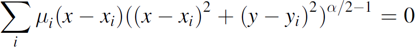
where μ_i is as defined for Equation (1), and d_i is the distance between nodes n₀ and n_i. We, therefore, need to minimize:

E = \sum_{i} E_{i}

(6)

Using the Pythagorean Theorem, calculus, and the fact that x and y are orthogonal, this value is a minimum when the following two equations are satisfied:

\sum_{i} μ_{i} (x - x_{i}) ((x - x_{i})^{2} + (y - y_{i})^{2})^{α / 2 - 1} = 0

(7)

\sum_{i} μ_{i} (y - y_{i}) ((x - x_{i})^{2} + (y - y_{i})^{2})^{α / 2 - 1} = 0

where, x_i and y_i are the coordinates of i^th node among the n nodes around the node n₀.

In [33], we considered only the case where α = 2, and the solution is a simple weighted average. This problem is easy to compute because the factor for x (y) that contains y (x) becomes a constant factor of 1.

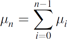
For other values of α, we have two equations with two unknowns. This can be solved using any number of root finding techniques, including Newton's method. In this paper, we used numerical methods to find the optimal position of the node when α is not 2.

Now, if we denote:

E_oci as the energy required for i'th node to communicate with its next node considering node ‘n_o’ in its original position. The sum of these values equals the remaining node energy, ignoring sensing and computation energy.

E_nci as the energy required for i'th node to communicate with its next node considering node ‘n_o’ in its expected new position, for the expected node lifetime in the original position.

E_conserved as the energy saved by moving the node to the new position, then

E_{c o n s e r v e d} = \sum_{i = 0}^{n - 1} (E_{o c i} - E_{n c i})

(8)

The energy required for a node to move distance d₁ is:

E_{m} = m^{*} d_{1}^{α}

(9)

where,

E_m is the energy required for movement

m is the energy required to move 1 unit

d₁ is the distance moved by the node in units

α is the RF attenuation factor

Nodes move only if:

E_{c o n s e r v e d} > E_{m}

(10)

(i.e., Nodes move only when it leads to an expected net energy savings). Since intermediate nodes forward packets to the next hop on the path to the user community:

μ_{n} = \sum_{i = 0}^{n - 1} μ_{i}

(11)

Node repositioning conserves energy in two ways:

It minimizes the energy needed for communications in a local neighborhood.

It allows nodes to move to positions that mitigate the impact when other nodes die.

There is a natural tendency for nodes to drift towards their data sink (closer to the edge of the terrain.) To slow this, we allow nodes to move only with probability p. Figures 9 through 11 illustrate a simulation scenario that shows how node repositioning implicitly tends to cause nodes to organize themselves into straight lines.

Figure 9.

Nodes at the beginning of a simulation.

Figure 10.

Over time nodes tend to form straight lines.

Figure 11.

As nodes die, other nodes move to mitigate the global impact.

In addition to reducing the migration of nodes to the terrain edge, p also reduces jitter. Nodes moving simultaneously to lower energy positions would cause oscillations, with nodes searching for optimal positions in response to neighbor movement. This would reduce the network lifetime. In some ways, this resembles the use of simulated annealing in [13]. Empirical testing found that the value of 0.3 for p worked best in our scenarios. Fiugre 12 shows results from simulations where p was varied. Figure 13 shows results obtained using numerical methods to find the optimal position for a node in a typical neighborhood. The top node is the data sink and the second node from the top is the node looking for its optimal position. The initial situation is given along with results when α is set to 2, 3, 4, and 5. This diagram reinforces the natural tendency of nodes to drift towards their data sink, since communications with the sink accounts for more than half of the total data traffic for the node. Figure 13 also indicates that the optimal position is not strongly influenced by α. As α increases the node is pulled more strongly towards the data sink, but this is not a very strong attraction.

Based on these results we suggest that scenarios where the attenuation factor is large are best served by approximating the optimal position by computing the weighted centroid, but weighing the data sink more heavily. This is simpler than solving equation (7) and likely to produce identical results. Based on these results, we also ignored the influence of α in the rest of our analysis. The only significant influence larger values of α will have is increasing the energy cost for data transmissions.

Simulation results

Figures 14 and 15 shows simulation results for lifetime extension simulations with p set to 0.3 and α set to 2. These values are used throughout the rest of this paper, based on our analysis shown by Figs. 12 and 13. Our model ignored multi-path fading and other environmental factors that affect communications reception, except for their implicit use in Equation (1).

Figure 12.

Mean network lifetime vs the number of nodes when nodes move with a fixed probability. (From top to bottom at position 1000: p = 0.3, 0.0, 0.1, 0.7, and 0.5).

Figure 13.

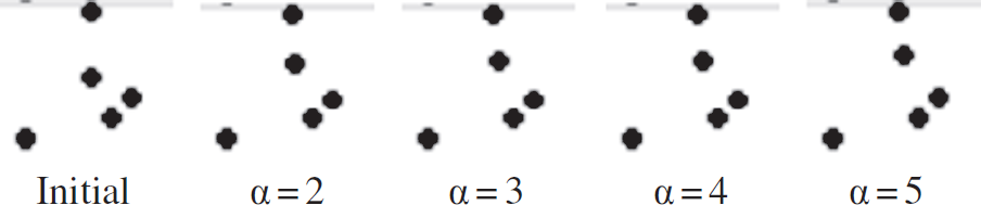
The second node from the top moves to its optimal position for varying values of α.

Figure 14.

Mean network lifetime versus the number of nodes when nodes are allowed to modify their position.

Figure 15.

Comparison of the results of this paper with those in [33].

In spite of its increased overhead, node relocation can effectively increase the lifetime of the network. Like data aggregation, this effect is noticeable even when the network consists of a relatively small number of nodes.

Figure 15 compares our current results with the results we presented in [33]. The difference between the two results is that the position used in the earlier work did not reflect the data transmission rates between individual nodes. Since the simulations place nodes at random and have targets move through the surveillance space using randomized trajectories, it seemed reasonable to assume that data rates would not have any discernable trends. As shown by both Equation (11) and Fig. 15, this assumption was erroneous. It is to be expected that this effect will be even more pronounced in actual applications where data traffic correlations are certain to exist. The use of mobile sensing nodes appears to be a useful energy savings technique that is frequently ignored in the literature.

The results from [33] are still interesting in that, although node repositioning without considering the data transmission rates appears to be of extremely limited utility, it worked well in combination with the other optimizations.

7. Combined Approaches

Figure 16 compares the optimization approaches presented in this paper. While data aggregation clearly has a more profound effect on prolonging network lifetime, the other two approaches also produce statistically significant results. Our interpretation of Fig. 16 is that by removing unnecessary communications, data aggregation reduces the energy overhead for networks of any node density. Repositioning nodes allows them to compensate for their uneven distribution in the surveillance region, which works well in moderately dense networks. When the network becomes dense, almost all nodes can use a relatively short communications range. Only at that point does adjusting the communications range result in truly significant energy savings.

Figure 16.

Mean network lifetimes versus number of nodes for the baseline and optimization approaches.

The rest of this section considers second-order effects. Figure 17 combines node range management with node movement. The results of this combination appear to have little synergy. It is almost as if a curve were constructed using the maximum values from the two individual optimizations.

Figure 17.

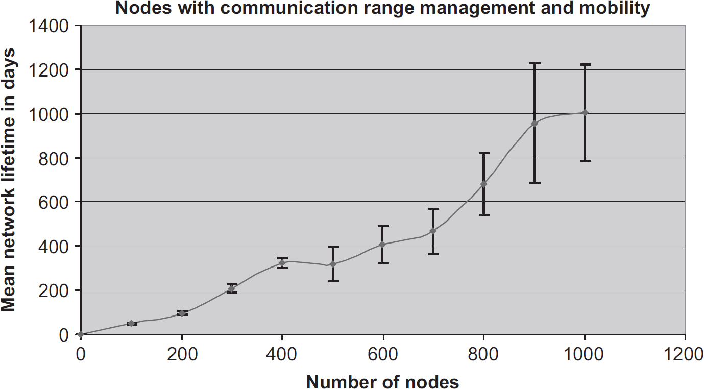
Mean network lifetime vs the number of nodes when communications range management and node relocation approaches are combined.

Figure 18 shows the results of combining node movement and local data agreement. There appears to be a real synergy that emerges when these approaches are combined. Note that the expected lifetime for large networks is nearly twice (triple) the expected network lifetime when data aggregation (node movement) is used in isolation. Interestingly, while the curve for both optimizations in isolation tends to flatten as the network size increases, over the range tested the network lifetime increase is almost linear.

Figure 18.

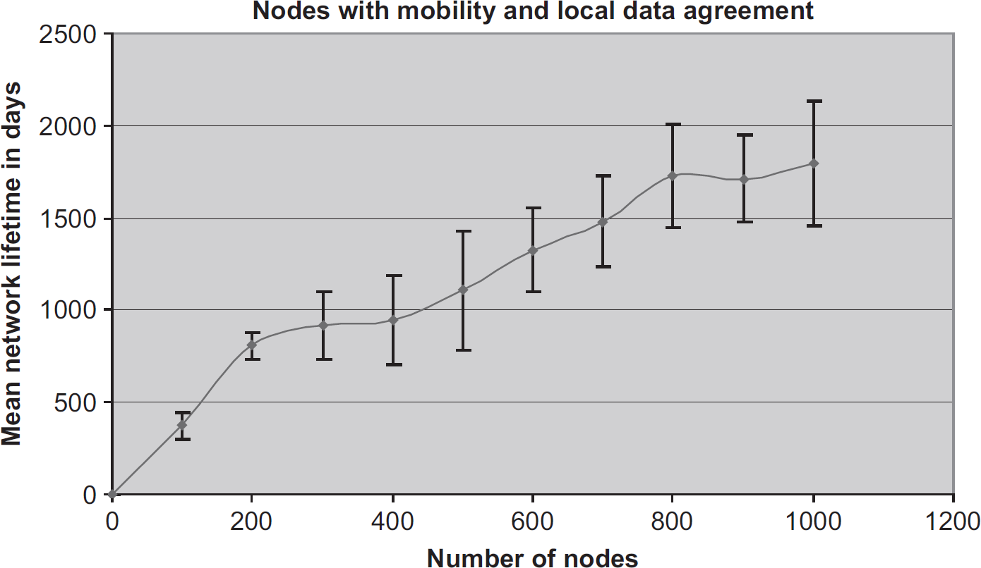
Mean network lifetime vs the number of nodes when we combined local data agreement and node relocation.

The most promising pairwise combination occurs when communications range management and local agreement are combined as shown in Fig. 19. This effectively quadruples the lifetime of the network when compared to either optimization in isolation. As with the optimization shown in Fig. 18, this synergy leads to a near linear increase in network lifetime over the range of node densities simulated.

Figure 19.

Mean network lifetime vs the number of nodes when we combined local data agreement and communications range management approaches.

Figure 20 shows the results of combining all three optimizations. The mean values in Fig. 20 are slightly better than the ones in Fig. 19, but the difference is within the error bars. While we believe this difference to be real, it is not statistically significant. This is partly due to the size of the confidence interval in Fig. 20 indicating that the amount of utility of this approach varies greatly from instance to instance. Figure 21 combines and summarizes these results. The combination of range management and data agreement is clearly more significant than any other pairwise combination. It also scales better with the network size.

Figure 20.

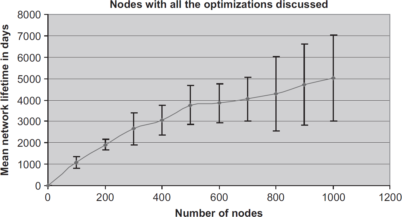
Mean network lifetime vs the number of nodes when the three optimizations are combined.

Figure 21.

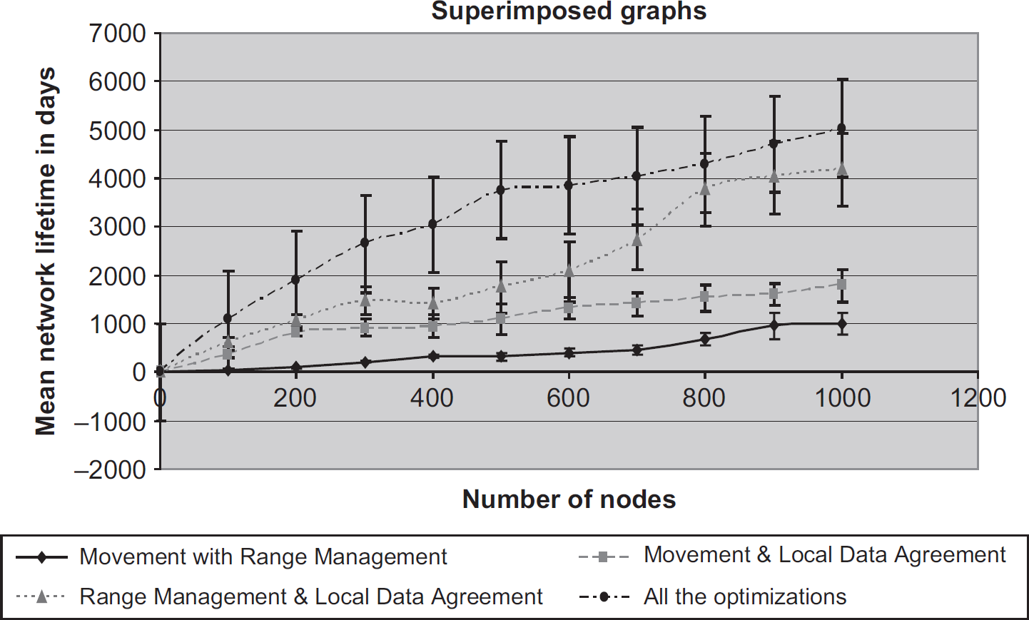
Combined approaches superimposed. (From bottom to top: range management with movement, data agreement with movement, data agreement with range management, and all three optimizations).

The results from [33] are shown in Fig. 22. The approaches used are identical, except that the data transmission rates were ignored when computing the optimal position for node relocation. In contrast with the results for optimizations in isolation, the results for node movement in combination with other optimizations are not significantly better when data transmission rates are considered. This answers a question that was posed by our analysis in [33], why does node relocation result in significant performance improvements only when combined with other optimizations? Node movement in isolation is not sufficient. The node movement is mainly useful as an enabling technology in combination with other methods to reduce network power consumption.

Figure 22.

Combined approaches superimposed ignoring packet rates at nodes.

8. Comparison with the Literature

The need for sensor networks to be parsimonious with power resources is well established. A common approach is for nodes to “sleep,” voluntarily transitioning into a semi-dormant low energy state as in [28]. Nodes interleave their active and dormant time slices extending the lifetime of the network at the cost of adding additional hardware. In essence, replacement nodes are pre-positioned in the field. We consider this concept orthogonal to the work presented here.

Much energy awareness research has concentrated on developing efficient networking technologies, like the efficient MAC protocol in [28]. The same research group also used data aggregation to reduce the volume of network traffic in [21]. However, the networking layer does not have sufficient application information to correctly aggregate multiple detections from multiple nodes into a single event, nor can it filter false positives from the system. Efficient routing methods have been developed, like the one in [12] that combines energy awareness and fault tolerance.

Non-network centered work has considered how to reduce power requirements at the hardware [26], operating system [25], and compiler [10] levels. The concepts presented here, while conscious of power constraints, are primarily situated at the applications layer and have possible synergies with all of these research efforts.

Few papers have considered issues involving sensor node movement to minimize power consumption. The approach in [11] uses integer linear programming to plot the routes for a node to minimize the combined cost of movement and data transmission. Unfortunately this approach requires prior knowledge of the node communications patterns, which is not feasible in surveillance applications.

The ideas in [13] are not dissimilar to the mobility approach presented here in that they look at issues concerning power consumption, network communications, and surveillance. In addition, the simulated annealing based ideas presented in that paper also consider the problems of multiple nodes moving simultaneously to optimize their position. Unlike our paper, [13] assumes that nodes will position themselves to continually survey targets in a specific location and arrange a store and forward network to support that application. We assume that targets are mobile and the communications patterns for detection information will be largely unpredictable.

9. Conclusions

This paper considered how local node adaptations extend the effective lifetime of a surveillance sensor network. We started by considering the criteria used to determine whether or not a network is viable. Considerations of network connectivity and sensor coverage ignore the ability of the network to perform its task. On the other hand, we find that the presence of a giant component in the system is a practical method for determining whether or not a surveillance network is functional.

We then consider how local adaptations can extend the effective lifetime of a network. They are preferable to centralized approaches, since they scale well as the network size increases. Allowing nodes to determine their own communications power, detection thresholds, and positions integrates communications, sensing, and applications considerations in our framework.

We demonstrate the performance of the network using each of these optimizations:

Communications range management reduces the power needed for transmitting information.

Node relocation reduces transmission power needs.

Data agreement reduces the volume of information transmitted.

We found that local data agreement provides the most significant improvement in network longevity. Communications range management is also useful, mainly significant for a larger number of nodes in the network. The combination of the two shows synergy between the two approaches. Although repositioning nodes to reduce the power needed for communications gives less improvement when compared to other techniques, when combined with other techniques it does significantly extend the network lifetime. When all optimizations are applied together, it extends the network lifetime to almost 25 times the baseline.

The data agreement approach could be combined with the ability to modify the detection threshold. This would allow nodes to increase their effective sensing region without excessively affecting network performance. In these tests we assumed that the effective sensing range is much larger than the communications range, which is typically the case. A fuller understanding is needed of the interactions between these two ranges and how they determine system performance.

References

Akyildizm

I. F.

Sankarasubramaniam

Cayirci

, “A survey on sensor networks,” IEEE Communications vol. 40, no. 8, pp. 102–114, Aug. 2002. http://www.cs.colorado.eduz/~rhan/CSCI_7143_001_Fall_2002/Papers/akyildiz02survey.pdf.

Bollobas

, Random Graphs. Cambridge University Press, Cambridge, 2001.

Brooks

Griffin

Friedlander

D. S.

, “Self-organized distributed sensor network entity tracking,” International Journal of High Performance Computer Applications, special issue on Sensor Networks, vol. 16, no. 3, 207–220, Fall 2002.

Brooks

R. R.

Ramanathan

Sayeed

, “Distributed target tracking and classification in sensor networks,” Proceedings of the IEEE, Invited Paper, vol. 91, no. 8, 1163–1171, August 2003.

Brooks

R. R.

Friedlander

Koch

Phoha

, “Tracking multiple targets with self-organizing distributed ground sensors,” Journal of Parallel and Distributed Computing Special Issue on Sensor Networks vol. 64, no. 7, pp. 874–884, August 2004.

Brooks

R. R.

, “Random networks and percolation theory,” Chapter 49. Distributed Sensor Networks, eds. Iyengar

S. S.

Brooks

R. R.

, pp. 907–946, Chapman & Hall/CRC Press, Boca Raton, FL, 2005.

Carman

D. W.

Kraus

P. S.

Matt

B. J.

, Constraints and Approaches for Distributed Sensor Network Security (Final), NAI Labs Technical Report #00–010, September 1, 2000.

Chen

Yao

, “Beamforming,” Chapter 56, Distributed Sensor Networks, (ed.s) Iyengar

S. S.

Brooks

R. R.

, pp. 1069–1106, Chapman & Hall CRC Press, Boca Raton, FL, Fall 2005.

Doherty

Warneke

B. A.

Boser

B. E.

Pister

K. S. J.

, “Energy and performance considerations for smart dust,” International Journal of Parallel and Distributed Systems and Networks vol. 4, no. 3, pp. 121–133, 2001.

10.

Kadayif

Kandemir

Choudhary

Karakoy

Vijaykrishnan

Irwin

M. J.

, “Compiler-directed communications energy optimizations for microsensor networks,” Chapter 36. Distributed Sensor Networks, eds. Iyengar

S. S.

Brooks

R. R.

, pp. 711–734, Chapman & Hall/CRC Press, Boca Raton, FL, 2005.

11.

Kadayif

Kandemir

Vijaykrishnan

Irwin

M. J.

“An integer linear programming based tool for wireless sensor networks”

Journal of Parallel and Distributed Computing, in press.

12.

Kannan

Iyengar

S. S.

, “Sensor centric routing in wireless sensor networks,” Ch. 37. Distributed Sensor Networks, eds. Iyengar

S. S.

Brooks

R. R.

, pp. 735–748, Chapman & Hall/CRC Press, Boca Raton, FL, 2005.

13.

Rao

Kesidis

, “Purposeful mobility for relaying and surveillance in mobile ad-hoc sensor networks,” IEEE Transactions on Mobile Computing vol. 3, no. 3, pp. 225–232, July–September 2004. http://labs.ee.psu.edu/faculty/kesidis/public_html/TMC2004.pdf.

14.

Krishanmachari

, “Phase transition phenomena in wireless ad hoc networks,” Golbecom 2001, San Antonio, TX, Nov. 2001, http://www.kroshnamachari.net/papers/phaseTransitionWirelessNetworks.pdf.

15.

Phoha

Brooks

, “Emergent Surveillance Plexus MURI Annual Report,” The Pennsylvania State University Applied Research Laboratory, Report 1, Defense Advanced Research Projects Agency and Army Research Office, (March 2002).

16.

Phoha

Brooks

, “Emergent Surveillance Plexus MURI Annual Report,” The Pennsylvania State University Applied Research Laboratory, Report 2, Defense Advanced Research Projects Agency and Army Research Office (March 2003).

17.

Potlapally

N. R.

Ravi

Ragbunathan

Jha

N. K.

, “Analyzing the energy consumption of security protocols,” Proc. International Symposium on Low Power Electronics and Design, pp. 30–35, 2003.

18.

Pottie

G. J.

Kaiser

W. J.

, “Wireless integrated network sensors,” Communications of the ACM vol. 43, no. 5, pp. 51–58, May 2000. http://portal.acm.org/citation.cfm?doid=332833.332838.

19.

Rabaey

J. M.

Ammer

Karalar

Otis

Sheets

Tuan

, “PicoRadios for wireless sensor networks: the next challenge in ultra-low-power design,” Proceedings of the International Solid-State Circuits Conference, San Francisco, CA, February 3–7, 2002.

20.

Roundy

Wright

P. K.

Rabaey

J. M.

, Energy Scavenging for Wireless Sensor Networks, Kluwer Academic Publishers, Amsterdam, 2004.

21.

Silva

Heidemann

Govindan

Estrin

, “Directed Diffusion,” Ch. 29. Distributed Sensor Networks, eds. Iyengar

S. S.

Brooks

R. R.

, pp. 573–596, Chapman & Hall/CRC Press, Boca Raton, FL, 2005.

22.

Slavin

Brooks

R. R.

Keller

, “A comparison of tracking algorithms using beamforming and CPA methods with an emphasis on resource consumption vs. performance,” PSU/ARL ESP MURI Technical Report, 2002.

23.

Stauffer

Aharony

, Introduction to Percolation Theory, Taylor & Francis, London, 2001.

24.

Swanson

D. C.

, “Environmental effects,” Ch. 11. Distributed Sensor Networks, eds. Iyengar

S. S.

Brooks

R. R.

, pp. 201–212, Chapman & Hall/CRC Press, Boca Raton, FL, 2005.

25.

Swaminathan

Chakrabarty

, Operating System Power Management,” Ch. 34. Distributed Sensor Networks, eds. Iyengar

S. S.

Brooks

R. R.

, pp. 667–696, Chapman & Hall/CRC Press, Boca Raton, FL, 2005.

26.

Vijaykrishnan

Irwin

M. J.

Kandemir

Chen

Kang

, “Designing energy aware sensor systems,” Chapter 33. Distributed Sensor Networks, eds. Iyengar

S. S.

Brooks

R. R.

, pp. 653–666, Chapman & Hall/CRC Press, Boca Raton, FL, 2005.

27.

Washburn

A. R.

, Search and Detection, 4th ed. INFORMS, Linthicum, MD, 2002.

28.

Wei

Heidemann

John

Estrin

Deborah

, “An Energy-Efficient MAC protocol for Wireless Sensor Networks,” in Proceedings of the IEEE Infocom, pp. 1567–1576. New York, NY, USA, USC/Information Sciences Institute, IEEE. June, 2002. <http://www.isi.edu/~johnh/PAPERS/Ye02a.html>.

29.

Zhao

Guibas

L. J.

, Wireless Sensor Networks: an information processing approach, Morgan Kaufmann, San Francisco, 2004.

30.

Zhu

Mengxia

Ding

Song

Brooks

R.R.

Qishi

Iyengar

S.S.

Nageswara

S.V. Rao

, “Decision making-based multiple sensor data fusion,” Submitted for review, 2005.

31.

Zou

Chakrabarty

, “A distributed coverage- and connectivity- centric technique for selecting active nodes in wireless sensor networks,” IEEE Transactions on Computers vol. 54, pp. 978–991,August 2005.

32.

Tian

Georganas

N. D.

, “A node scheduling scheme for energy conservation in large wireless sensor networks,” Wireless Comm. Mob. Comput. vol. 3, pp. 271–290,2003.

33.

Brooks

R. R.

Siddul

, “On adaptation to extend the lifetime of surveillance sensor networks,” Innovations and Commercial Applications of Distributed Sensor Networks Symposium, Bethesda, MD (October 2005).

Adaptive Optimizations for Surveillance Sensor Network Longevity

Abstract

Keywords

1. Introduction

2. Network Vialbility Criterion

5.1. Baseline Simulations

9. Conclusions

References