Sage Journals: Discover world-class research

Abstract

An energy efficient cover of a region using Wireless Sensor Networks (WSNs) is addressed in this paper. Sensor nodes in a WSN are characterized by limited power and computational capabilities, and are expected to function for extended periods of time with minimal human intervention. The life span of such networks depends on the efficient use of the available power for sensing and communication. In this paper, the coverage problem in a three dimensional space is rigorously analyzed and the minimum number of sensor nodes and their placement for complete coverage is determined. Also, given a random distribution of sensor nodes, the problem of selecting a minimum subset of sensor nodes for complete coverage is addressed. A computationally efficient algorithm is developed and implemented in a distributed fashion.

Numerical simulations show that the optimized sensor network has better energy efficiency compared to the standard random deployment of sensor nodes. It is demonstrated that the optimized WSN continues to offer better coverage of the region even when the sensor nodes start to fail over time. A localized “self healing” algorithm is implemented that wakes up the inactive neighbors of a failing sensor node. Using the “flooding algorithm” for querying the network, it is shown that the optimized WSN with integrated self healing far outweighs the performance that is obtained by standard random deployment. For the first time, a “measure of optimality” is defined that will enable the comparison of different implementations of a WSN from an energy efficiency stand point.

Keywords

Sensor Networks 3D Coverage 3D Deployment Optimality Ad-hoc Networks Energy Efficiency

1. Introduction

Advances in wireless communication and low-cost sensors have made possible the design and deployment of large-scale wireless sensor systems. These Wireless Sensor Networks (WSNs) have found applications in target classification and tracking [1 –3]; health applications [4]; and in environmental and ecological monitoring [5–6]. Such networks are increasingly deployed in buildings, underwater, on roads or bridges, and in planetary exploration. Most existing results focus on planar networks [14 –24]; however, a three-dimensional modeling of the sensor network would reflect more accurately the real-life situations. Some applications of the results presented in this paper are:

Disaster Recovery: Natural disasters (floods, hurricanes, and fires) require sensing in different planes and thus 3-dimensional coverage techniques are required. Three-dimensional networks also arise in building networks where nodes are located on different floors.

Mapping Topographical Properties: Random dense sensor deployment on irregular terrains like mountains and hills leaves three dimensional coverage holes that indicate the topographical properties of the terrain. Understanding the topography of an area enables the understanding of watershed boundaries, drainage characteristics, water movement, impacts on water quality, and soil conservation. The detecting of the coverage holes is also a critical military application because it determines the ability of armed forces to take and hold areas, and to move troops and material into and through areas. Topographical properties can also be useful in determining weather patterns.

Space Exploration [7–8]: Wireless sensor networks will play an important role in planetary explorations. A rover functioning as a base station collects measurements and relays aggregated results to an orbiter.

Undersea Monitoring [9 –11]: Underwater sensor deployment enables the real time monitoring of selected ocean areas. Under Water Acoustic Sensor Networks (UW-ASN) can consist of a number of sensors and submersible vehicles that are deployed to perform collaborative monitoring tasks over a given area.

A very limited number of the applications mentioned afford the flexibility in placing sensor nodes at desired locations for optimum coverage. In a majority of the applications, the nodes are randomly distributed, for example dropped from an airplane, onto the region to be monitored. The sensing needs in each of these applications are fundamentally different and require the use of different types of sensors, each with a different sensing range and sensitivity. A sensor node typically has numerous sensors and can be configured to monitor the region and transmit the information back to a sink. The number of sensor nodes required depends on the size of the region to be covered, the sensing radius of the node, and the type of coverage desired. The information is transmitted to a sink typically through multi-hop communications in the WSN. The impact of the number of nodes on the capacity of multi-hop wireless networks was analyzed for deployments in two dimensions [12] and three dimensions [13]. Under a protocol model of non-interference, if n nodes, each with a transmission rate of W bits/second, are randomly distributed in a disc of area A sq. meters (m²), then the throughput obtained by each node for transmission to a randomly chosen sink is given by $Θ (\frac{W}{\sqrt{n \log n}})$ bits / sec [12]. Similarly in the three dimensional deployment of wireless nodes, the throughput achieved when n nodes are located in a sphere of volume V is given by $Θ (\frac{W}{\sqrt{{(n \log^{2} n)}^{1 / 3}}})$ bits / sec [13]. Since the number of active nodes depends on the type of sensing required and the region of coverage, the overall communication and energy efficiency of the WSN can be significantly improved by optimizing the number of nodes while guaranteeing the coverage of a region.

The coverage of a two dimensional surface by planar WSNs was studied in the past. Gupta and Das [14] introduced the notion of a “connected sensor cover” and the energy efficiency was addressed through the construction of a near-optimal connected sensor cover. The problem of selecting a subset of randomly deployed nodes for energy efficiency and coverage of an area was also addressed by Cardei [15] and Slijepcevic [16]. Energy efficiency is improved by selecting those sensor nodes having the largest area of coverage and then placing the remaining nodes in a low energy state. Marengoni [17] and de Berg [18] address the placement of sensor nodes in the context of an “art gallery” problem where every point in the region of interest is covered by at least one sensor node. Sensor placement for surveillance and target location was also addressed by Chakrabarty [19] and Dhillon [20]. Approximate algorithms for coverage were proposed in [21] and results from computational geometry were used to determine completeness of coverage of a region by the WSN [22 –24]. The problem of selecting a minimum number of nodes such that each node in the network is either selected or is a neighbor of a selected node was formulated as the minimum dominating connected set (MDCS) problem [25]. In [26], Chen and Liestman proposed an algorithm for finding small weakly-connected dominating sets in a WSN. Shakkottai [27] derived the necessary and sufficient conditions for the connectivity and coverage in terms of the sensing radius, transmission radius, and the failure rates of the nodes. The connectivity issue was also addressed as the problem of selecting k-basestations out of a given set of n basestations [28]. Voronoi diagrams and graph search techniques were utilized in [29 –31] to design robust, efficient, and scalable algorithms to be used in the integration of WSNs.

In recent years, sensor systems deployed on mobile robots have seen increased usage. The coverage issues in such systems were first addressed by Gage [32]. Here three types of coverage that arise in mobile WSNs (blanket, barrier, and sweep coverage) were defined. Three dimensional deployments of sensor nodes were also studied in the context of underwater Maximization of the swept coverage [33], while the problem of adequate coverage and connectivity in mobile WSNs was addressed in [34]. Zhang and Hou [34] show that if the communication range is at least twice the sensing range, then a complete coverage of a convex area implies connectivity among the nodes. A Coverage Configuration Protocol (CCP) that can provide different degrees of connected coverage is presented in [35]. The energy consumption issue in WSNs has primarily been approached from a communication standpoint [36 –38]. Here, the focus has been the determination of optimum sleep and wake times for the sensing nodes.

In this paper, the energy efficiency of a WSN is studied in the context of the coverage of a region using wireless sensor nodes. First, the minimum number of sensor nodes required to cover a three-dimensional region is determined and an algorithm for testing the coverage of a sensor network is proposed. A computationally simple method for selecting a minimum subset of a random distribution of sensor nodes for coverage is then developed. This method is implemented in a distributed fashion across the WSN and the saving obtained is analyzed. Using the standard flooding algorithm [39 –41], the performance of the optimized network is shown to be superior to the performance of the original deployment. A localized “self healing” algorithm is also implemented that wakes up the inactive neighbors of a failing sensor node. It is shown that the performance of the optimized WSN with integrated self healing far outweighs the performance that is obtained by standard random deployment. For the first time, a “measure of optimality” is defined that will enable the comparison of different implementations of a WSN from an energy efficiency stand point.

The rest of the paper is organized as follows. The coverage problem in WSNs is formulated in Section 2. The minimum number of sensor nodes needed to cover a 3D region is determined in Section 3. In Section 4, an algorithm for the selection of a minimum set of sensor nodes to guarantee coverage is developed. The connectivity and power efficiency issues are addressed in Section 5. In Section 6, an algorithm for checking the extent of coverage for a known deployment is presented. Numerical simulation results that validate the proposed algorithms are presented in Section 7 and the conclusions and future work are summarized in Section 8.

2. Problem Analysis

A wireless sensor network consists of a large number of wireless sensor nodes either placed at specific locations or distributed randomly in a region. The first step in implementing such a sensor network is to determine the coverage of the sensor nodes. To accomplish this, the notions of sensing region and coverage are first defined and the coverage and optimization problems are then formulated. Since in practice, a large number of sensor nodes are distributed randomly in the region to be monitored, the sensing and communication regions of all the nodes are assumed to be identical. It is also assumed that the region to be monitored is large in comparison to the sensing region of an individual node and that the locations of all the nodes are known. The discussion in this paper assumes the ability of each node to detect the phenomenon of interest. The actual sensed value, sensor fusion, and routing of the information to a sink, while of enormous importance, are beyond the scope of the present work.

2.1 Mathematical Preliminaries

Let O be the output of a sensor node S that is capable of sensing a phenomenon P. Let S have a sensing radius R_s and a communication radius R_c.

Definition 2.1

The phenomenon P located at Y ∈ R³ is said to be detectable by sensor S located at X ∈ R³ if and only if there exists a constant threshold δ > 0 such that O(Y) > δ if the phenomenon ‘P’ is present. The quantity ‘δ’ is the signal threshold and is specific to the type of sensor used.□

The sensing region of sensor node S located at X(x,y,z) is the collection of all points where the phenomenon P is detectable by the sensor node S, i.e. A = {y ∈ R³ | P is detectable by S}. While the sensing region of an individual node can depend on the sensor and the environment it is deployed in, it is necessary to have a simplified representation of the sensing region to reduce the computational complexity in determining the coverage of a WSN. In this paper, we will restrict the sensing region of S to be an open ball centered at X ∈ R³.

Definition 2.2

Let Y = {y ∈ R³ | O(y) > δ}. The sensing region of sensor node S located at X ∈ R³ is defined as A = {y ∈ Y ‖ y - X ‖ ≤ R_s}, where ‖·‖ is the Euclidean distance between y and X.

$R_{s} (= min_{Y | O (y) > δ} ∥ Y - X ∥)$ in this definition is the radius of the open ball representing the sensing region and is called the sensing radius of S.

2.2 Problem Formulation

Consider a network comprising of sensor nodes S₁,…,S_n, each with a sensing radius equal to R_s. Let A_i be the sensing region of node S_i and ‘R’ the region to be monitored. Then, given the collection of nodes C_n = {S₁,…,S_n}, the sensing region of this collection can be expressed as $\bar{C_{n}} = \cup_{i = 1}^{n} A_{i}$ .

Definition 2.3

A collection of sensor nodes C_n = {S₁,…,S_n}is said to cover the region R if and only if $R \subseteq \bar{C_{n}}$ .□

If C_n covers R, then $p \in R \Rightarrow p \in A_{i}$ for some S_i ∈ C_n. This is commonly referred to in literature as the 1-cover of the region R. A natural extension of 1-cover is k-cover where any point in the region belongs to the sensing regions of at-least k nodes. In this paper, a cover is interpreted as the 1-cover of the region.

The coverage and deployment problems in WSNs can be addressed by studying the following two sub-problems:

Problem 1(Optimal Deployment): Find the minimum number of sensor nodes and their locations to cover a given region R.

Problem 2(Reduced Coverage): Given a dense deployment of sensor nodes, find a reduced subset of active nodes that guarantee coverage of R.

3. Optimal Deployment

The concept of an optimum cover is introduced in this section. In a deployment of sensor nodes, if the number of the sensor nodes and their locations can be specified, then it is possible to find the exact location for each sensor node in order to cover the region using the smallest number of nodes. Such a deployment is optimal. On the other hand, given a random distribution of the sensor nodes, it is possible to activate only a subset of the nodes and still maintain cover of the region. A reduced cover is a set of sensor nodes that completely cover the region and removal of any node in this set leads to loss of coverage. In this section, the problem of determining the optimum cover is addressed by solving the related problem of packing a volume with equal overlapping spheres. In order to achieve this, the notion of “thickness” of a cover is first defined along the lines in Conway [43]. When flexibility in deployment exists, it is advantageous to find an optimum deployment of the sensors so that complete coverage can be achieved using a minimum number of sensors. The deployment strategy proposed in this section achieves optimum coverage by modeling the coverage region of each sensor by a sphere and then determining the optimum way to cover the desired region with equal overlapping spheres. In order to achieve this, the notion of “thickness” of a cover is first defined.

Definition 3.1

The thickness θ of a cover is defined as the averages number of spheres that contain a point of the space i.e. $θ = \frac{V o l u m e o f o n e s p h e r e}{V o l u m e o f f u n d a m e n t a l r e g i o n} = \frac{\frac{1}{n} \sum_{i = l}^{n} V_{i}}{\frac{1}{n} V_{t o t a l}} = \frac{n V}{V_{t o t a l}}$ where “n” is the number of active sensor nodes; V_i is the volume of sensing region of sensor node S_i; and V_total is the total volume of the sensed region R.

Definition 3.2

The covering radius, R_cover, of spheres centered at X₁, X₂,…,X_n is the minimum sensing radius that will cover the region R.

The deployment problem in WSNs can now be addressed as the problem of determining the thinnest cover of a region R by sensor nodes S₀, S₁….,S_k. In a 3-dimensional space the best (thinnest) covering of spheres known [42, 43] is when the centers of the spheres are at the vertices of a body centered cubic lattice (bcc lattice). Given the sensing radius R_s of each sensor, the optimal spacing between the centers of each sphere forming a new lattice Λ’ is constructed in the following manner.

Define Λ’ as the bcc lattice covering the region R. For this Lattice, let R_cover be the covering radius.

Define $α = \frac{S e n s i n g R a d i u s o f e a c h n o d e}{C o v e r i n g R a d i u s} - \frac{R_{s}}{R_{c o v e r}}$

The new lattice ΛÁ is obtained as α.Λ

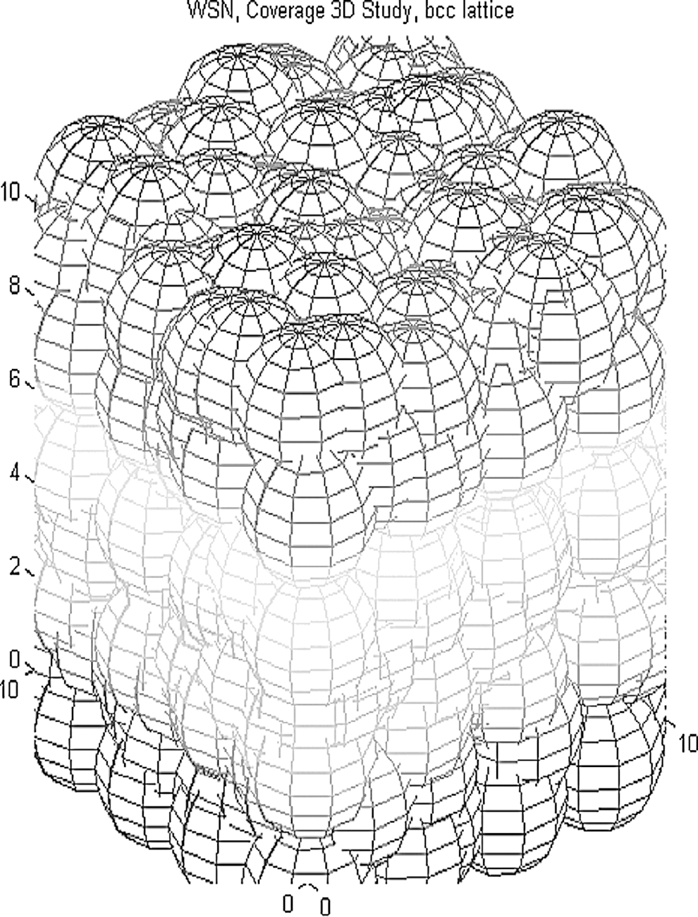
This implies that arranging the sensor nodes with their centers coincided with the vertices of this lattice, Λ′, will guarantee an optimal covering of the region spanned by this lattice. The minimum number of sensor nodes required to cover the region R is the minimum number of vertices of the Lattice that cover the region R. The spacing of the lattice is a function of the sensing radius of the sensor node. The covering radius of a bcc lattice is. $R_{c o v e r} = \frac{\sqrt{5}}{2} = 1.1180$ . Moreover, the thickness of such a cover is $θ = \frac{5 π \sqrt{5}}{24} = 1.4635$ . The optimal deployment of sensor nodes for coverage of a 3D region is shown in Fig. 1.

FIGURE 1

Deployment strategy in 3D using bcc Lattice arrangement of 128 nodes. The coverage region is 10 units × 10 units × 10 units and the sensing radius is 1.5 units.

4. Reduced Coverage

In practice, given an existing distribution of sensors, it is often necessary to minimize the number of sensor nodes that remain active while still achieving complete coverage of the entire region. In this section, an algorithm is developed where the nodes make local decisions on whether to sleep, or join the set of active sensors. If the sensing region of a sensor node is completely covered by its neighbors, then the sensor can be disabled without affecting the overall coverage. Thus, by iteratively disabling sensors that are covered by other sensors, one can arrive at a reduced set of sensors that guarantee a 1-cover of the desired region. Since the approach is iterative in nature, the solution that is arrived at is not necessarily an optimum one. Thus, for the algorithm to be truly useful, it is necessary to also have a means to compare it to the optimal solution in order to ascertain the effectiveness of the proposed algorithm. In this section, a rigorous mathematical proof of the proposed technique is provided along with a metric to compare the performance of the reduced network with the optimum coverage obtained in Section 3.

The central point of the algorithm is that the nodes make local decisions on whether to sleep, or join the set of active nodes. If the sensing region of a node is completely covered by its neighbors, then the node can be disabled without affecting the overall coverage.

Let C_n = {S₀, S₁, S₂,…,S_n} be the set of all the sensor nodes that cover the region R. Let the intersection of sphere S₀ and sphere S_i be given by the circle C_i, i.e. C_i = A₀ ∩ A_i (Fig. 2). The interior of the circle C_i is said to be the disc bounded by the circle C_i, i.e. D_i = interior (C_i). A circle C_i is completely covered if the disc bounded by the circle is completely covered, i.e. $\forall p \in D_{i}, p \in \underset{\begin{matrix} j = 1 \\ j \neq i \end{matrix}}{\cup} A_{j}$ .

FIGURE 2

Intersection of two sensing regions.

Theorem 4.1

Let the sensor node S₀ be adjacent to sensor nodes S₁, S₂,…, S_n and C_k = A₀ ∩ A_k, k − 1‥n be the circles of intersection. S₀ is completely covered if and only if all C_k′ s,k = 1‥n are covered.

Proof

If S₀ is completely covered, then every disc D_k in S₀ is covered. The definition of complete coverage of a disk ensures that the “if” part of the theorem holds.

Conversely, suppose every disc D_k in S₀ is covered. Then, ∀ p ∈ D_k, p ∈ D_l where l ∈ [l,…,k-I, k+l,…n]. Now, if S₀ is not covered, then there is a point q ∈ S₀ ∈ q ∋ D_k, k − 1,‥,n. This implies that the point ‘q’ is exterior to the circle segments that bound each D_k. Since ‘q’ is not covered, there is at least one circle segment that is not covered. This contradicts the assumption that all the circles of intersection are covered. Therefore, if all the circles of the intersection are covered, then S₀ is covered. □

The utility of Theorem 4.1 is in reducing the coverage of sensor node S₀ to a simpler problem of checking if all the circles of the intersection between S₀ and the adjacent nodes are covered. This still is a complex task that is difficult to achieve in real time. The following theorem demonstrates a technique where such coverage can be determined by a few straightforward computations.

Theorem 4.2

A circle C₀ is completely covered by spheres if all the intersection points C_i ∩ C_j ∈ D₀, ∀i, j = 1…n are covered by one or more adjacent spheres.

Proof

Consider an uncovered point ‘p7’ in D₀. Since some parts of D₀ are covered by adjacent sensor nodes, these spheres are going to partition D₀ into regions bounded by arcs from the boundary of C₀ and/or arcs from circles. C_k′ s, k = 1…,n Suppose ‘p’ belongs to a region R_x in D₀. Since ‘p’ is not covered, it is easy to see that R_s has to be bounded only by the exterior arcs of the circles. Also, the entire boundary of R_x, including the intersection points of the arcs, must have the same coverage status as ‘p’, i.e. all the intersection points on the boundary of R_x in D₀ must not be covered. This contradicts the assumption that all the intersection points C_i ∩ C_j ∈ D₀, ∀i, j = 1…n are covered. Therefore, if all the intersection points C_i ∩ C_j ∈ D₀ are covered by one or more adjacent spheres, then D₀ is covered. Consequently, C₀ is covered.
4.1 Algorithm for Obtaining Reduced Coverage

Theorem 4.1 and 4.2 indicate that a sensor node is completely covered if all the intersection points C_i ∩ C_j ∈ D_k are covered by some sensor S_l, l ≠ i, j, k = 1‥n. Therefore, to check if S₀ is completely covered, one has to first find all the circles obtained by the intersection of S₀ ∩ S_k, k = 1‥n. For each C_k, find all the intersection points that lie within D_k. If all these intersection points are covered, then the circles C_k are covered. Then, by the theorems 4.1-4.2, S₀ is covered and can be deactivated. The following definitions aid in this process.

Definition 4.1

A sensor S_i is said to be a neighbor of sensor S_j if and only if d(X_i, X_j) ≤ 2R_c, where R_c is the communication radius of sensors S_i and S_j.

Definition 4.2

The neighbor set N(i) of sensor S_i is the set of all the neighbors of sensor S_i and is defined as N(i) = {S_j ∈ C | d(X_i, X_j) ≤ 2R_c; j = 1,‥,n, j ≠ i}. |N(i)| is the cardinality of set N(i) i.e. the number of neighbors of sensor S_i.

Selection Algorithm for Complete Coverage

Step 1. For each node Si, form the set of neighbors. N(i). For each element ‘S_k’ in N(i) compute the volume of overlap, V_ik, between sensor node S_i and S_k. If the total overlap between S_i and its neighbors is less than the volume of S_i, then S_i is not completely covered by its neighbors and must remain active. That is $V_{o v e r l a p} = \sum_{k = 1}^{n} V_{i k} \leq \frac{4}{3} π R s^{3} \Rightarrow S_{i}$ remains active.

Step 2. $V_{o v e r l a p} \geq \frac{4}{3} π R s^{3}$ does not necessarily mean that S_i is covered. To check if S_i is covered, for every pair of nodes S_j, S_k in N(i) do the following:

Find C_ij the circle got by the intersection of the coverage surface of S_i, S_j.

Find C_ik the intersection circle of S_i, S_k.

Find the intersection points C_ij ∩ C_ik.

If the intersection points are all covered, i.e. C_ij ∩ C_ik ∈ A_l, S_l ∈ N (i), l ≠ i,j,k, then deactivate S_i.

It is well known that the coverage problem in WSNs is NP-hard [17]. The computational complexity of the algorithm developed in this section is O(N³) where $N = ({m a x}_{i - 1}^{n} | N (i) |)$ is the maximum number of nodes in the neighbor set of any sensor in the network.

Definition 4.3

The measure of optimality of a WSN is the ratio of the number of active sensors in the network to the minimum number of sensors that can completely cover the same region.

The results in Section 3 show that the optimum deployment of sensors in 3D would result in sensors located at the vertices of a bcc lattice. Therefore, given the region to be monitored, one could easily find the number of sensors required and their location for complete coverage. However, if the sensors are already deployed and a subset of these sensors selected to keep active, then the measure of optimality is a measure of excess energy spent in monitoring the region as compared to an optimum deployment of the sensors. A network with a lower “measure of optimality” would result in lesser expenditure of energy in monitoring the region.

The main advantage of this algorithm is that it is low in computational complexity and is executed in a distributed manner. The algorithm requires that each sensor node knows the locations of all its neighbors. The neighbor list can be easily compiled by the nodes based on the “HELLO” messages exchanged at start up. When a network is deployed, all nodes are initially active. As the algorithm progresses, redundant nodes will switch to the inactive mode until no more nodes can be turned off without causing a hole in the coverage. To avoid neighbor nodes running the algorithm simultaneously and causing a “blind spot,” each node announces to its neighbors that it is currently running the coverage algorithm. If the node is redundant and is eligible for turning off without affecting the overall coverage, it will broadcast a “GOODBYE” message to its neighboring nodes. Neighboring nodes receiving such a message will delete the sender's information from their neighbor lists.

5. Connectivity in 3D Wireless Sensor Networks

Consider a WSN comprising of sensor nodes S₁…‥S_n with sensing radius R_s, and communication radius R_c, respectively. Let R be the region to be monitored. Denote the sensing and communication regions of a sensor node S_i as A_is and A_ic respectively.

Let $\bar{C} = ⋃_{i = 1}^{i = m} A_{i s}$ and $\overset{=}{C} = ⋃_{i = 1}^{i = m} A_{i c}$ be the sensing space and communication space of a set of nodes C = {S₁, S₂,…S_m} respectively. □

Definition 5.1

A set of nodes C_a = {S_a1,‥,S_am} is said to be connected if for every $a, b \in {\overset{=}{C}}_{a}$ there exists a continuous function $f : [0, 1] \to {\overset{=}{C}}_{a}$ such that, f (0) = a; f (1) = b, and $\forall t \in (0, 1), f (t) \in {\overset{=}{C}}_{i}$

Connectivity implies that the location of any active sensor node is within the communication range of one or more active nodes such that all the active nodes form a connected communication backbone, while coverage requires all locations in the coverage region to be within the sensing range of at least one active node. Obviously, the relationship between coverage and connectivity depends on the ratio of sensing radius to communication radius. In the two dimensional case, it was shown that coverage implies connectivity whenever the radius of communication is twice the radius of coverage [34–35]. This result can be trivially extended for coverage and connectivity in three dimensions. □

Lemma 5.1

A necessary and sufficient condition to ensure that coverage implies connectivity in 3D is that the radius of communication be at least twice the sensing radius.

If the condition of Lemma 5.1 holds, then complete coverage automatically implies connectivity. Therefore, the connectivity problem is not explicitly addressed in this paper.

6. Checking for Coverage in a WSN

This section presents a simple algorithm for testing the coverage obtained in a wireless sensor network. This algorithm tests for coverage by generating an occupancy grid and checking if each cell in this grid is covered by at least one node. The entire region is covered if all the cells in the grid are covered. This test will also help determine the degree of the cover and, in the case of incomplete coverage, the “size” of the holes. The degree of the cover is the least number of sensor nodes that cover any point in the region and is a measure of redundancy in the WSN. Redundant active nodes are indicative of the excess energy expended in a WSN. The information on the size and location of the holes in the coverage helps determine the number of additional nodes required and their placement to guarantee complete coverage.

The coverage problem in this paper is initially posed as a problem of covering a 2D region with equal, overlapping disks. The region of interest is first partitioned into a grid with a spacing of 0.5R_s. An origin is arbitrarily assigned and successive cells are numbered. An occupancy matrix (column vector) is then formed and initialized to zero. Every cell in the region is referenced by one entry in the occupancy matrix. For each node in the network, the covered cells are determined and the cells in the occupancy matrix corresponding to the covered cells are indexed by ‘1’. A zero entry in the occupancy matrix indicates an uncovered cell in the region. The number of uncovered cells and their locations can then be used to determine the size and locations of the uncovered regions. Further, since the cell entries in the occupancy matrix are indexed, an entry ‘k’ indicates that the cell is covered by ‘k’ sensor nodes. Thus the smallest entry in the occupancy matrix gives the degree of the cover.

The grid generated is the smallest grid entirely covering the region R. If R is smaller than the grid, then only the relevant cells in the grid can be chosen for testing the coverage. This is done by assigning ‘X’, i.e. do not care, to cells that are outside the desired region of coverage. In the three dimensional case, the region is divided into cubes of side 0.5R_s and the coverage of each cube is verified by checking the distance between the node and the center of the cube.

A grid spacing of 0.5R_s implies that a sensor node can cover a maximum of 25 cells in two-dimensional space and 125 cubes in a three-dimensional space (Fig. 3). Therefore, for a network containing ‘n’ sensor nodes, this algorithm requires O(n) steps to verify if the region is completely covered. The algorithm presented is simple and easy to implement. It not only determines the extent of coverage but also identifies the size and location of the holes in the coverage.

FIGURE 3

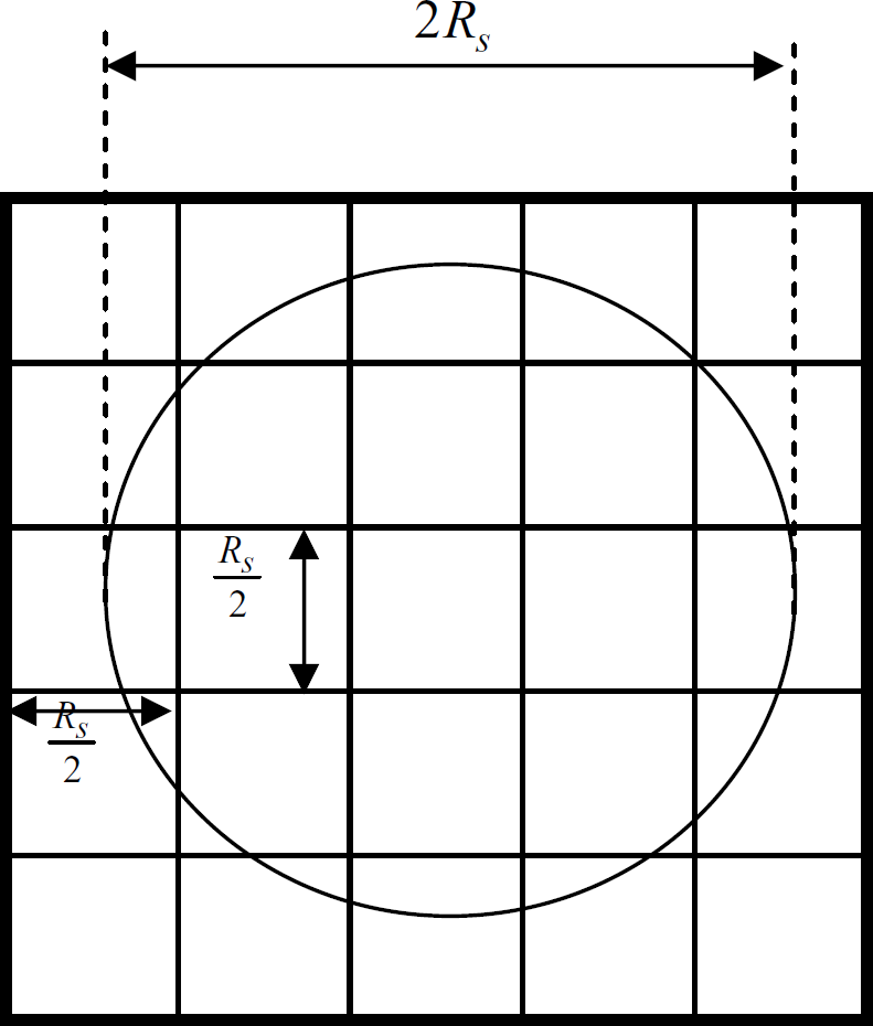
The coverage region of a sensor node.

7. Numerical Results

The theoretical developments in Sections 2–6 are validated through numerical examples in this section. First the case of random deployment of sensor nodes is studied and compared to the optimum deployment. In the second case, given a deployment of sensor nodes, a reduced cover is obtained.

Example 1

In this example, the number of sensor nodes required to cover a 3D region of size 10 × 10 × 10 units is considered. Table 1 shows the comparison of the number of nodes required for coverage using random deployment and deployment using a bcc lattice. In Fig. 4, the required number of nodes with different sensing radii using random deployment and bcc lattice deployment are compared. Since low cost, low power sensor nodes typically have a small sensing radius, the random deployment of such nodes requires the use of a very large number of nodes. Therefore, efficient deployment of such sensor nodes requires a technique for determining a reduced subset of sensor nodes from a randomly deployed set of nodes.

FIGURE 4

Number of sensor nodes required (with different sensing radii) for coverage of a 10 × 10 × 10 region under different deployment strategies: Random Deployment and bcc lattice deployment with different sensing radii.

TABLE 1

Number of sensor nodes required for coverage of a 10 × 10 × 10 region under different deployment strategies

Sensing Radius	Random Deployment	bcc lattice Deployment
2	182	54
1.5	325	128
1	773	396
0.6	2228	1421
0.3	24551	10952

The sensor nodes were distributed randomly using a uniform distribution over the entire region of interest. The structure obtained under bcc lattice deployment is shown in Fig. 2. Figure 2 gives some insight into the placement of sensor nodes in three dimensional deployment of WSN, especially in buildings [45] and in underwater applications [9–10].

Example 2

In this example, the optimum coverage algorithm described in Section 4 is used to find the reduced cover of region 10×10×10 units when sensor nodes are randomly deployed. The nodes have a sensing radius of 1 unit and initially 2000 nodes are randomly deployed in this region using a uniform distribution. Figure 5(a) shows the initial deployment of the nodes and Fig. 5(b) shows the reduced cover obtained by the algorithm in Section 4. It can be seen that 422 nodes were active in the reduced cover resulting in savings of 78.9%. If a bcc lattice deployment was used, then the minimum number of sensor nodes required would be 396. 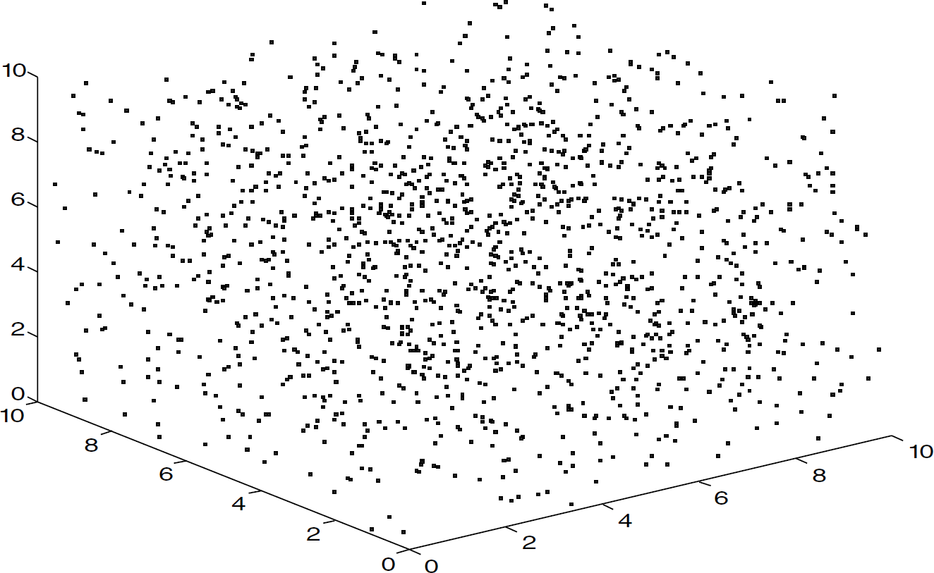Therefore, the reduced cover has a measure of optimality equal to 1.06, which indicates that the algorithm has resulted in a solution very close to the optimum cover that is obtained by bcc lattice deployment.

FIGURE 5a

Random distribution of 2000 sensor nodes over a region 10 × 10 × 10 units.

FIGURE 5b

Reduced cover of the region 10 × 10 × 10 units. Initial Deployment = 2000; Number of active nodes = 422.

Example 3

The goal of this example is to compare the occupancy matrix before and after running the coverage algorithm. In this example, the optimum coverage algorithm described in Section 4 is used to find the reduced cover of region 10×10×10 units when sensor nodes are randomly deployed. The nodes have a sensing radius of 2 units and initially 2000 nodes are randomly deployed in this region using a uniform distribution. A 3D grid (grid size=one unit) is generated and 1000 grid points are tested for coverage. Figure 6 shows the occupancy matrix of each grid point in the initial deployment of the sensor nodes compared to that after running the coverage algorithm. Table 2 displays the minimum and maximum number of sensor nodes covering a cell in the grid before and after running the coverage algorithm. It can be seen that after running the algorithm a maximum of 5 sensor nodes cover any cell in the grid. The degree of cover after running the algorithm is 1, which guarantees that the region is completely covered.

FIGURE 6

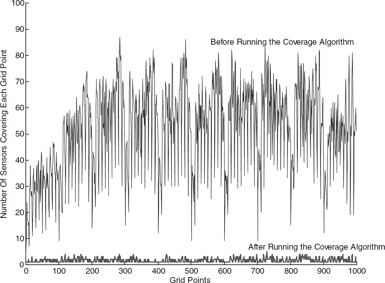
1000 Grid points were tested, Sensor Radius = 2, Grid Size = 1, Occupancy Matrix - Initial Deployment (top) and after running the algorithm (bottom).

TABLE 2

Comparing the minimum and maximum cover before and after running the algorithm

	Min. Cover	Max. Cover
Before	8	89
After	1	5

Example 4

In this example, the minimum number of nodes that are required for random deployment is studied. In Example 3, 2000 nodes, each with a sensing radius of 1 unit, were randomly deployed to cover a region of 10×10×10 units. The optimum cover of this region required 396 nodes resulting in 1,604 inactive nodes. In order to determine the number of sensor nodes required to cover the region, a number of trials were conducted and the resulting coverage was analyzed. The number of holes in the coverage for 10 trials is shown in Fig. 7. It is seen that at least 800 nodes are required to adequately cover the region when random deployment is used. The reduced cover algorithm therefore results in a saving of 48%.

FIGURE 7

10 different trials of a random 3D deployment of sensor nodes on a 10 × 10 × 10 region and the resulting holes in the coverage.

Example 5

The reduced cover of a deployment is obtained by first establishing communications between nodes to establish the list of neighbors and then iteratively executing the algorithm at each node. Therefore, the communication overhead increases as the number of deployed nodes increase. Figure 8 shows the average number of messages over 10 trials for the different number of deployed nodes. From this figure, it can be seen that the communications overhead for the initialization of the network increases exponentially with the increase in deployed nodes. The advantage of using a reduced cover is further demonstrated by comparison of the performance of the flooding algorithm both in the original deployment, as well as in the reduced WSN. The number of messages for different queries is shown in Fig. 9. It can be seen that the flooding algorithm results in a fewer number of messages in the reduced network.

FIGURE 8

Effect of the number of deployed nodes on the number of messages between the nodes.

FIGURE 9

Number of queries vs. number of messages in a WSN - (i) Initial deployment (Flooding Algorithm); (ii) Reduced deployment (Coverage Algorithm).

The performance of the over time was also studied to determine the benefits of using a reduced cover. This is done by assuming that each sensor node has a limited energy supply of 300 Joules and is deactivated when the available energy is used up. The performance is evaluated in terms of coverage lifetime. The coverage lifetime is the continuous operational time of the system before the coverage drops below a specified threshold (for example 0.8). The nodes are assumed to consume 1400mW for each transmission and 1000mW for each reception. Further, the nodes are assumed to consume 830mW, 130mW in the idle and sleep states respectively. Figures 10a and 10b show the overall coverage obtained over time as the WSN processes a series of queries. In these figures, two different initial deployments of 800 and 1600 nodes are considered. It can be seen in both the cases that the overall coverage drops over time as the available energy is used in processing the queries. Using the reduced network, it is seen that the resultant cover over time is significantly better. This is because each node in the reduced network has fewer neighbors and as a result has more efficient communications and less energy expenditure per query. This improvement in the coverage lifetime comes at a cost. The algorithm for obtaining the reduced network requires the communication between a node and its neighbors and as a result a portion of the energy is used up during the initialization stage of the network. This causes early onset of degradation and loss of cover. This, however, can be addressed by incorporating self healing in the WSN.

FIGURE 10a

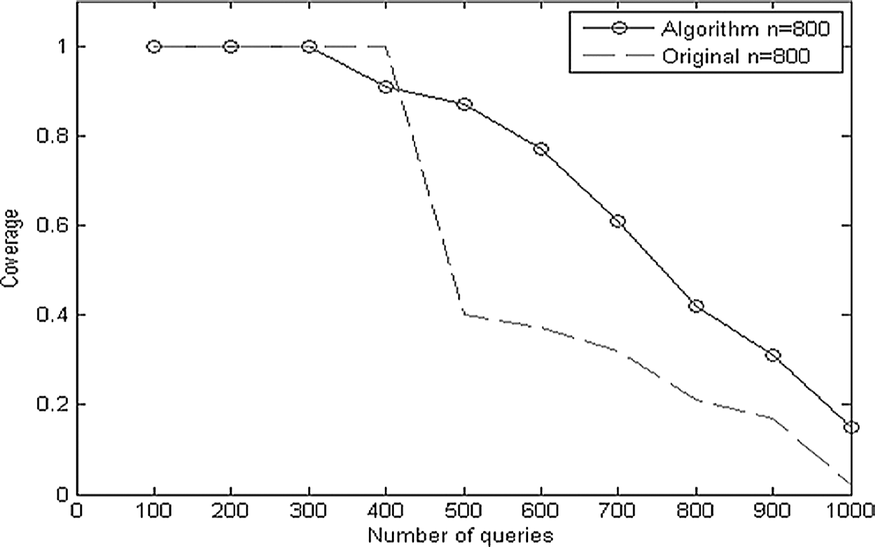
The effect of number of queries on the coverage lifetime of the WSN with 800 nodes - (i) Initial deployment (Original); (ii) Reduced deployment (Algorithm).

FIGURE 10b

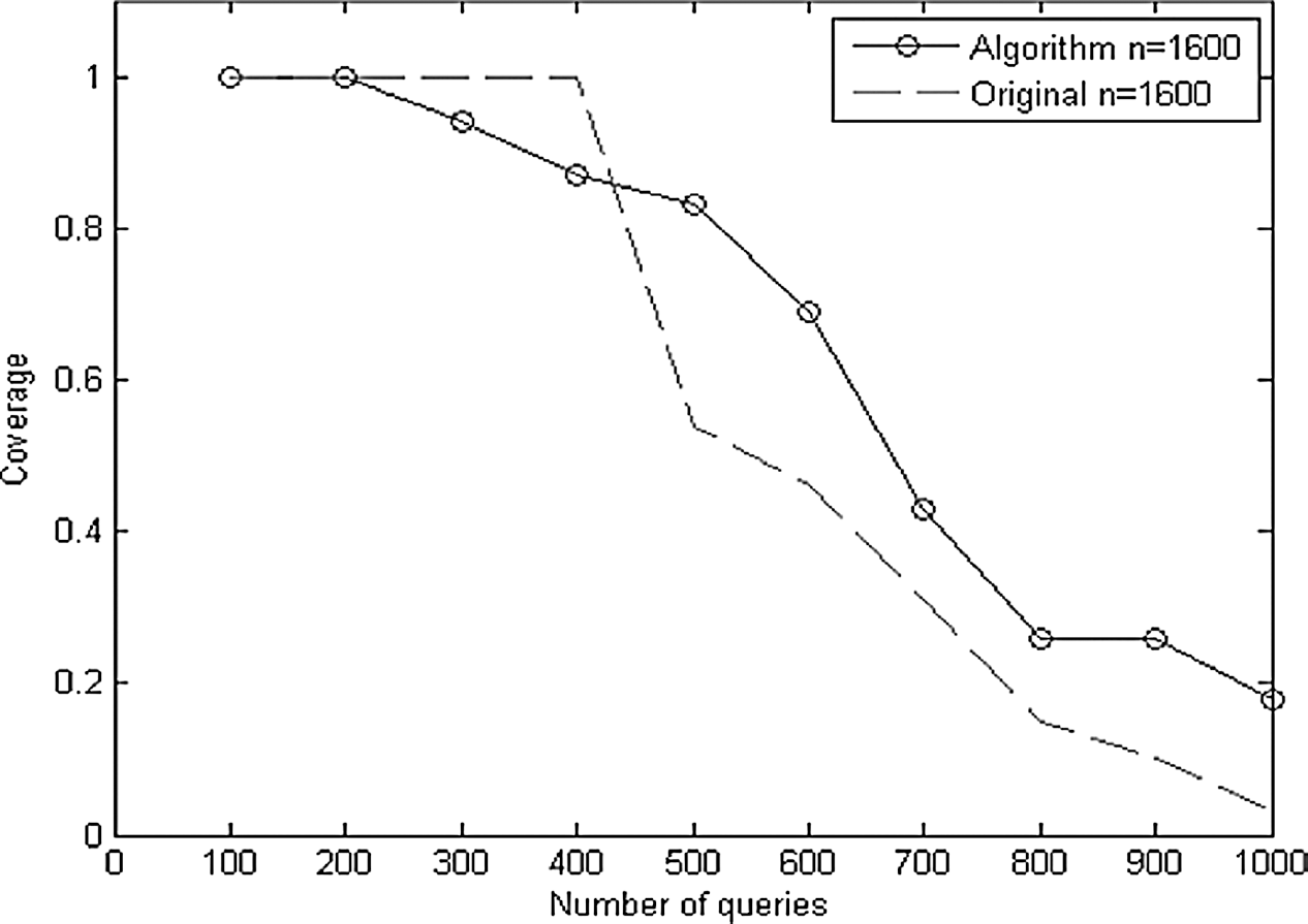
The effect of number of queries on the coverage lifetime of the WSN with 1600 nodes - (i) Initial deployment (Original); (ii) Reduced deployment (Algorithm).

To demonstrate the effect of self healing, a simple mechanism is implemented where a failing node in a reduced network alerts its neighbors about the impending failure. Inactive nodes in the neighborhood of the failing node are then activated. Since the inactive nodes and the failing node have overlapping cover, activating all the neighbors improves the coverage and results in better lifetime coverage for the WSN. The performance of the WSN for initial deployments of 800 and 1600 nodes with self healing is shown in Figs. 11a and 11b. Two different simulations are depicted in these figures, and in both the experiments the reduced network with self healing can be seen to outperform the original network. The self-healing algorithm presented is a simple extension of the results presented in this paper. A more elaborate self-healing algorithm is a topic of our future work [46].

FIGURE 11a

The effect of number of queries on the coverage lifetime of a self healing WSN with 800 nodes - (i) Initial deployment (Original); (ii) Reduced deployment (Algorithm).

FIGURE 11b

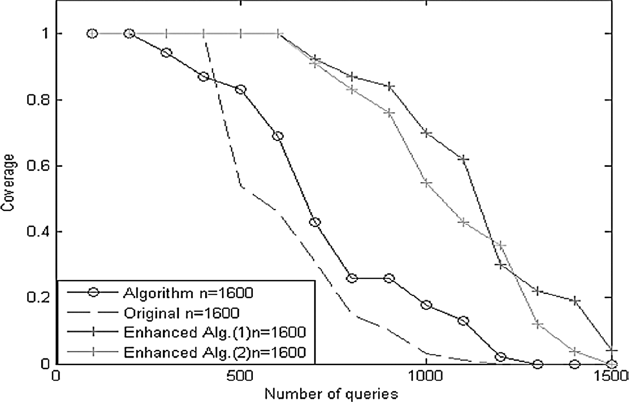
The effect of number of queries on the coverage lifetime of a self healing WSN with 1600 nodes - (i) Initial deployment (Original); (ii) Reduced deployment (Algorithm).

8. Conclusions and Future Work

Energy efficient coverage of a region using Wireless Sensor Networks (WSNs) was addressed in this paper. The main contribution of this paper is a technique for obtaining a reduced cover of a wireless sensor network. The technique is shown to be computationally simple and suitable for distributed implementation. Numerical simulations show that the reduced sensor network has better energy efficiency compared to the random deployment of sensor nodes. It was demonstrated that the reduced WSN continues to offer better coverage of the region even when the sensor nodes start to fail over time. A localized “self healing” algorithm is implemented that wakes up the inactive neighbors of a failing sensor node. Using the “flooding algorithm” for querying the network, it is shown that the reduced cover of the WSN with integrated self healing offers superior performance over time. For the first time, a “measure of optimality” has been defined that enables the comparison of different implementations of a WSN from an energy efficiency stand point.

The proposed algorithm is computationally simple and will result in lower communication overhead. The 3D coverage algorithm can be easily extended to obtain application specific reduced cover, border coverage for intrusion detection, to determine the mobility of sensor nodes to cover sensing holes, and to incorporate self-healing in sensor networks. Practical ways of 3D deployment for tracking applications is part of our ongoing and future research. In this paper, the sensing region of each sensor node was assumed to be a disk (2D) or an open ball (3D). This model is a simplification motivated by the need for analysis. This model, while useful, is still simplistic and does not address the realities in practical implementations. Signal to Noise ratio (SNR) in sensing, multi-path, and fading issues in communications between the nodes, and data fusion are all important aspects that affect the functioning of a WSN and will be investigated in our future work. Our future work also evaluates the performance of our algorithms based on different sensing models and the design of hybrid coverage protocols capable of delivering accurate spatio-temporal profile of different kinds of sensing measurements.

Footnotes

Acknowledgements

The authors gratefully acknowledge the assistance of the U.S. Department of Defense, Army Research Office, in supporting this work through grant # DAAD 19-03-1-0142. The authors would also like to thank Prof. Sridhar Radhakrishnan, School of Computer Science, University of Oklahoma, for his valuable comments and suggestions. The authors would also like to thank the anonymous reviewers for their suggestions in improving the quality of the presentation.

References

Aslem

Butler

Constantin

Crespi

Cybenko

, and Rus

, “Tracking a moving object with a binary sensor network,” in Proceedings of the 1^st International Conference on Embedded Networked Sensor Systems, Los Angeles, California, November 2003, pp. 150–161.

Fang

Zhao

, and Guibas

, “Lightweight sensing and communication protocols for target enumeration and aggregation,” in Proceedings of the 4^th ACM International Symposium on Mobile Ad Hoc Networking & Computing (MobiHoc), 2003, pp. 165–176.

Galstyan

Krishnamachari

Lerman

Pattem

, “Distributed online localization in sensor networks using a moving target,” in Proceedings of the 3^rd International Symposium on Information Processing in Sensor Networks, Berkeley, California, USA, 2004, pp. 61–70.

Schwiebert

Gupta

S. K. S.

, and Weinmann

, “Research challenges in wireless networks of biomedical sensors,” in Proceedings of Mobile Computing and Networking Conference, Rome, Italy, July 2001, pp. 151–165.

Bhardwaj

Garnett

, and Chandrakasan

A.P.

, “Upper bounds on the lifetime of sensor networks,” in Proceedings of IEEE International Conference on Communications ICC'01, Helsinki, Finland, vol. 3, June 2001, pp. 785–790.

Bulusu

Estrin

Girod

, and Heidemann

, “Self-configuring localization systems: Design and Experimental Evaluation,” ACM Transactions on Embedded Computing Systems (TECS), vol. 3, (1) Feb. 2004, pp. 24–60.

Hong

Gerla

Bagrodia

Estabrook

Kwon

, and Pei

, “The mars sensor network: Efficient, power aware communications,” in Proceedings of IEEE Military Communications Conferences (MILCOM 2001), McLean, VA, October 2001.

NASA/JPL Sensor Webs Project, http://sensorwebs.jpl.nasa.gov/.

Akyildiz

Pompili

, and Melodia

, “Underwater acoustic sensor networks: Research challenges,” Ad Hoc Networks (Elsevier), vol. 3, pp. 257–279, May 2005.

10.

Pompili

and Melodia

, “Three-Dimensional routing in underwater acoustic sensor networks,” in Proceedings of the 2^nd ACM International Workshop on Performance Evaluation of Wireless Ad Hoc, Sensor, and Ubiquitous Networks, October 2005, pp. 214–221.

11.

Proakis

J. G.

Sozer

E. M.

Rice

J. A.

, and Stojanovic

, “Shallow water acoustic networks,” IEEE Communications Magazine, vol. 39, pp. 114–119, 2001.

12.

Gupta

and Kumar

P. R.

, “The capacity of wireless sensor networks,” IEEE Transactions on Information Theory, vol. 46, pp. 388–404, March 2000.

13.

Gupta

and Kumar

P. R.

, “Internet in the sky: The capacity of three dimensional wireless networks,” Communications in Information and Systems, vol. 1, pp. 33–49, January 2001.

14.

Gupta

Das

S. R.

, and Gu

, “Connected sensor cover: Self-Organization of sensor networks for efficient query execution,” in Proceedings of MobiHoc 03, Annapolis, Maryland, USA, June 2003, pp. 189–200.

15.

Cardei

MacCallum

Cheng

Min

Jia

, and Du

D.-Z.

, “Wireless sensor networks with energy efficient organization,” Journal of Interconnection Networks, vol. 3, pp. 213–229, March 2000.

16.

Slijepcevic

and Potkonjak

, “Power efficient organization of wireless sensor networks,” in Proceedings of IEEE International Conference on Communications, vol. 2, 2001, pp. 472–476.

17.

Marengoni

Draper

Hanson

, and Sitaraman

, “System to place observers on a polyhedral terrain in polynomial time,” Image & Vision Computing Journal, vol. 18, pp.773–780, 2000.

18.

de Berg

van Kreveld

Overmans

, and Schwarzkopf

, “Computational Geometry: Algorithms and Applications,” Springer-Verlag, 2000.

19.

Chakrabarty

Iyengar

S. S.

and Cho

, “Grid coverage for surveillance and target location in distributed sensor networks,” IEEE Transactions on Computers, vol. 51(12), December 2002, pp. 1448–1453.

20.

Dhillon

S. S.

and Chakrabarty

, “Sensor placement for effective coverage and surveillance in distributed sensor networks,” in Proceedings of IEEE Wireless Communications and Networking Conference, 2003, pp. 1609–1614.

21.

Kar

and Banerjee

, “Node placement for connected coverage in sensor networks,” in Proceedings of WiOpt: Modeling and Optimization in Mobile, Ad hoc and Wireless Networks, Sophia-Antipolis, France, March 2003.

22.

Bonnimann

and Goodrich

, “Almost optimal set covers in finite vc-dimension,” Discrete & Computational Geometry, vol. 14, (4), pp. 463–479, 1995.

23.

Kumar

V. S. A.

Arya

, and Ramesh

, “Hardness of set cover with intersection,” in Proceedings of the 27^th International Colloquium on Automata, Languages and Programming, 2000, pp. 624–635.

24.

Kumar

V. S. A.

and Ramesh

, “Covering rectilinear polygons with axis-parallel rectangles,” in Proceedings of the 31^st Annual ACM Symposium on Theory of Computing, Atlanta, Georgia, 1999, pp. 445–454.

25.

Guha

and Khuller

, “Approximation algorithms for connected dominating sets,” in Proceedings of the Fourth Annual European Symposium on Algorithms, 1996, pp. 179–193.

26.

Chen

and Liestman

, “Approximating minimum size weakly-connected dominating sets for clustering mobile ad-hoc networks,” in Proceedings of the 3rd ACM International Symposium on Mobile Ad hoc Networking & Computing, Lausanne, Switzerland, 2002, pp. 165–172.

27.

Shakkottai

Srikant

, and Shro

, “Unreliable sensor grids: coverage, connectivity and diameter,” in Proceedings of IEEE INFOCOM, San Francisco, CA, vol. 2, 2003, pp. 1073–1083.

28.

Lieska

Laitinen

, and Lahteenmaki

, “Radio coverage optimization with genetic algorithms,” in Proceedings of IEEE International Symposium on Personal, Indoor, and Mobile Radio Communications (PIMRC), vol.1, 1998, pp. 318–322.

29.

Huang

Richa

, and Segal

, “Dynamic coverage and related problems in ad-hoc sensor networks,” ACM Mobile Networks and Applications, vol. 10, pp. 9–17, 2005.

30.

Wan

, and Frieder

, “Coverage in wireless ad-hoc sensor networks,” IEEE Transactions on Computers, vol. 52, pp. 753–763, June 2003.

31.

Meguerdichian

Koushanfar

Potkonjak

, and Srivastava

M. B.

, “Coverage problems in wireless ad-hoc sensor networks,” in Proceedings of the 20^th IEEE INFOCOM, 2001, pp. 1380–1387.

32.

Gage

D. W.

, “Command control for many-robot systems,” in Proceedings of the 19^th Annual AUVS Technical Symposium, pp. 22–24, 2002.

33.

Howard

Mataric

M. J.

, and Sukhatme

G. S.

, “Mobile sensor network deployment using potential fields: A distributed, scalable solution to the area coverage problem,” in Proceedings of the 6^th International Symposium on Distributed Autonomous Robotics Systems, 2002, pp. 299–308.

34.

Zhang

and Hou

J. C.

, “Maintaining sensing coverage and connectivity in large sensor networks,” Ad Hoc & Sensor Wireless Networks, an International Journal, vol. 1, UIUCDCS-R-2003–2351, June 2003.

35.

Wang

Xing

Zhang

Pless

, and Gill

C. D.

, “Integrated coverage and connectivity configuration in wireless sensor networks,” in Proceedings of the 1^st International Conference on Embedded Networked Sensor Systems, Los Angeles, California, USA, 2003, pp. 28–39.

36.

Cerpa and Estrin

, “Ascent: Adaptive Self-configuring Sensor Networks Topologies,” IEEE Transactions on Mobile Computing, vol. 3, pp. 272–285, July 2004.

37.

Heinzelman

W. R.

Chandrakasan

, and Balakrishnan

, “Energy-efficient communication protocol for wireless microsensor networks,” in Proceedings of the International Conference on System Sciences (HICSS), 2000.

38.

Zheng

Tao

Radhakrishnan

Sridhar

, and Sarangan

Venkatesh

, “PMAC: An adaptive energy-efficient MAC protocol for wireless sensor networks,” IEEE IPDPS, vol. 13, (13), pp. 65–72, April 2005.

39.

Tseng

Chen

, and Chen

, “The broadcast storm problem in a mobile ad hoc network,” Annual ACM/IEEE International Conference on Mobile Computing and Networking, Seattle, Washington, USA, Aug. 1999, pp. 151–162.

40.

Lim

and Kim

, “Multicast tree construction and flooding in wireless ad-hoc networks,” in Proceedings of ACM Modeling, Analysis, and Simulation of Wireless and Mobile Systems, Boston, Massachusetts, USA 2000, pp. 61–68.

41.

Basagni

Chlamtac

, and Bruschi

, “A mobility-transparent deterministic broadcast mechanism for ad hoc networks,” IEEE/ACM Transactions on Networking (TON), vol.7, pp.799–807, December 1999.

42.

Toth

G. Fejes

Kuperberg

, and Kuperberg

, “Highly saturated packings and reduced coverings,” Monatsh Math., vol. 125, (2) pp.127–145, 1998.

43.

Conway

J. H.

and Sloane

N. J. A.

, “Sphere Packings, Lattices and Groups,” Springer-Verlag, New York, 2nd ed., 1993.

44.

Megudio

and Tamir

, “On the complexity of locating linear facilities in the plane,” Operations Research Letters, pp.194–197, 1982.

45.

Center for Information Technology Research in the Interest of Society (CITRIS) program, http://www.coe.berkeley.edu/labnotes/1101smartbuildings.html.

46.

Commuri

and Watfa

, “Self healing sensor cover in wireless sensor networks,” ACM Transactions on Sensor Networks (TOSN), submitted, September 2005.

Coverage Strategies in Wireless Sensor Networks

Abstract

Keywords

1. Introduction

2. Problem Analysis

2.1 Mathematical Preliminaries

Definition 2.1

Definition 2.2

2.2 Problem Formulation

Definition 2.3

3. Optimal Deployment

Definition 3.1

Definition 3.2

Theorem 4.1

Proof

Theorem 4.2

Proof

Definition 4.1

Definition 4.2

Selection Algorithm for Complete Coverage

Definition 4.3

5. Connectivity in 3D Wireless Sensor Networks

Definition 5.1

Lemma 5.1

6. Checking for Coverage in a WSN

Example 1

Example 2

Example 3

Example 4

Example 5

Footnotes

Acknowledgements

References