
Abstract
Sensor networks consist of wireless enabled sensor nodes with limited energy. As sensors could be deployed in a large area, data transmitting and receiving are energy consuming operations. One of the methods to save energy is to reduce the communication distance of each node by grouping them in to clusters. Each cluster will have a cluster-head (CH), which will communicate with all the other nodes of that cluster and transmit the data to the remote base station. In this paper, we propose an extension to Growing Self-Organizing Map (GSOM) and describe the use of evolutionary computing technique to cluster wireless sensor nodes and to identify the cluster-heads. We compare the proposed method with clustering solutions based on Genetic Algorithm (GA), an extended version of Particle Swarm Optimisation (PSO) and four general purpose clustering algorithms. This could help to discover the clusters to reduce the communication energy used to transmit data when exact locations of all sensors are known and computational resources are centrally available. This method is useful in the applications where sensors are deployed in a controlled environment and are not moving. We have derived an energy minimisation model that is used as a criterion for clustering. The proposed method can also be used as a design tool to study and analyze the cluster formation for a given node placement.
Introduction
A sensor network is a network of several sensors, deployed in an ad hoc fashion to gather and transmit information. Sensor networks are becoming popular with the recent advancement in the area of low power electronics and radio frequency communication. Developments in sensor technology and communications suggest that future sensors can be extremely small as well as wireless enabled. The advances in sensor technology have a strong impact on the way data is sensed. Other factors that contribute to the growth of studies in sensor network are the ease of deployment, cost effectiveness, flexibility, and reliability. The major challenge in designing sensor networks is the amount of energy dissipated in the network. The energy used may be a combination of the processing energy, transmission energy, and receiving energy.
Managing and controlling sensors is a challenging problem in the defense, space, and manufacturing field. Let us consider a scenario where sensors are used to measure the tension in mechanical bolts. A potential application is the analysis of strain of a structure that is fitted with a large number of tension measuring bolts [1]. By forming sensor clusters, the tensions can be monitored remotely and necessary precautions can be taken when the need arises, instead of checking each bolt manually intermittently. In this type of application, the communicating sensors are static and the networking of this type of sensors is called static sensor networks [2]. As the number of sensors used in this application is very large, we can make the energy usage more economical by not allowing each sensor to transmit the information to the remote base station, but instead delegating few sensors to gather the information from other sensors and transmit to the base station [3]. In the example explained above, the sensors are placed in a pre-defined location, thus the positions of the sensors are always known in advance and sensors are stationary after deployment. The base station, which acts as a data-gathering unit is a powerful computer located generally in a remote location, far from the network. The base station does not have energy constraints as it is connected to the external power supply. Due to this advantage, base station should be used to do the computation intensive tasks. In this paper, we are discussing the optimization method which uses the base station resources to minimize the communication energy dissipation in the network based on clustering concept.
The rest of the paper is organized as follows. Section 2 describes the problem we are trying to solve in this paper and the assumptions we have made. Section 3 provides the details of the energy minimization model used to calculate the energy dissipation in the network. In section 4, Clustering techniques employed, including the algorithm we propose in the paper are presented. Section 5 gives the simulation and analysis of results. Section 6 concludes the paper.
Problem Definition
Clustering is a widely used method to improve the performance of wireless sensor networks. Clustering is used for a variety of purposes in wireless sensor network applications. Clustering is used for data fusion [4], routing, and optimizing energy consumption [3]. It is used effectively to increase the lifespan of a sensor network by minimizing the communication energy. In LEACH [5], communication between sensor nodes will occur, after each round is established. In each round, clusters are formed and cluster-heads are identified in a random manner. In LEACH-C [6], a centralized algorithm identifies the cluster-heads in each round. Formation of clusters and identifying cluster-heads will have a significant role in reducing the overall communication energy in sensor networks. In LEACH-C, a solution to the NP-hard problem[7] of finding optimal “K” clusters using simulated annealing approach is presented. When we have prior knowledge of the position of sensors deployed in a sensor networks, it is always worthwhile to cluster the sensors and allow few cluster-heads to communicate with the base station instead of all the sensors communicating with the base station. In this scenario, since the positions of all the sensors are known, a centralized algorithm should be used to cluster the sensors so that “K” optimal clusters are always formed in the network. This kind of sensor network can be used in a scenario where we have complete control over the deployment of the sensors, and thus know the position of all the sensors in advance. The main applications of these kinds of sensor networks are surveillance and monitoring. In this paper we have looked into the problem of cluster formation and cluster-head identification using energy minimization as the clustering criterion. We propose an extension to Growing Self-Organizing Map (GSOM) and applied it to cluster the sensor network. We are adopting an extended version of Particle Swarm Optimization (PSO) and the Genetic Algorithm (GA) approach to form clusters and identify cluster-heads. We have also used a conventional clustering algorithm like K-mean, Fuzzy C-mean, and subtractive clustering to compare the results of our proposed clustering algorithm.
The following are assumptions we have made in this study:
Each sensor node has a fixed omni directional transmission range. All the nodes have identical transmission ranges and hardware configurations. Nodes are distributed in a sensor field of 2-Dimension. The area of the problem space is known in advance. Once the nodes are deployed they are static and the position of the nodes is known to the base station beforehand. The base station runs the clustering algorithm and updates the nodes about their cluster-head. The sensor network is densely populated with minimum of 100 nodes in the network.
When the sensor nodes are deployed, our objective is to cluster the nodes and identify the cluster-heads (CH) using centralized algorithm so that CH can transmit data from their respective clusters to the base station. The algorithm developed in the paper can also be used as an analytical design tool to identify clusters and cluster-heads given the placement of sensors. This tool could be useful in studying the cluster formation and CH placement given the node positions. This is an application of a control environment where sensors are deployed when and where it is necessary.
There are a number of clustering algorithms used for wireless sensor and ad hoc networks in various contexts [8][9]. Their main aim is to generate a minimum number of stable clusters. Most of the clustering algorithms do not consider energy minimization of the network as criterion for clustering.
Minimization of Energy Usage
The important component of each sensor is a data and control processing unit and radio for communication. The microprocessor used in the processing unit should be energy efficient with less energy consumption. The energy dissipation in a radio depends on different characteristics of the radio. In this paper we are using a free-space simple radio model where energy consumed to transmit a data is square of the transmission distance.
Energy model
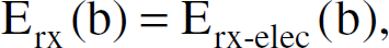
The energy model derived in this work is adopted from [10][3]. We have used the simple radio model to measure the energy dissipation to transmit and receive the data from the node. The energy dissipation for transmitting b (bits) to d (distance) is shown in (2),


The energy dissipation for receiving b bits of data is given in (4)
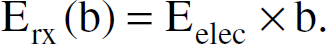
For our experiments, the transmission/receiver energy loss (Eelec) per bit is taken as Eelec = 50nJ / bit, and the transmission amplifier constant is taken has ∊amp = 0.1nJ / bit / m2 [3].
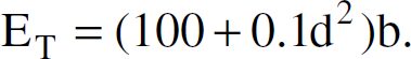
Energy consumption of a wireless sensor node transmitting and receiving data from another node at a distance “d” can be divided into two main components: energy used to transmit, receive, and amplify data ET, and energy used for processing the data Ep, mainly by the microcontroller. ET can be derived as
Ep has two components the energy loss due to switching, and the energy loss due to leakage. It can be shown that Ep is a function of the supply voltage V and the frequency f associated with the sensor. By experiment, we can find out the average capacitance Cavg switched per cycle, and the average number of clock cycles needed for the task Ncyc for a given microprocessor [11]. Therefore, total capacitance switched is Ncyc ∗ Cavg assuming I0 as the leakage current:

The total energy loss (E) of the sensor:

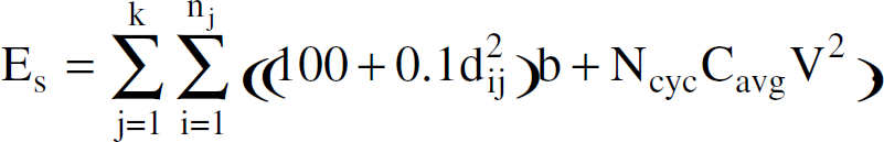
Assume a k set of sensor clusters with nj sensors in the cluster Cj, where l<j<k, as the energy optimized network architecture of a randomly distributed ntotal number of sensors, where

Considering the cluster Cj, in which a sensor Sij is at distance dij to the cluster-head CHj, and CHj has the distance Dj to the base station, the energy loss of all the sensors can be derived using (7). Leakage currents Io can be as large as few mA for microcontroller, and the effect of leakage currents can be neglected for higher frequencies and lower supply voltages. Assuming the leakage current Io as negligible, (7) can be simplified further [12]. Energy used by all k cluster-heads Ek

Energy used by all the other sensors Es
From (9) and (10) the total energy loss for the sensor system (Etotal) is:

In order to study the optimization with the first part of (11), we can further simplify (11). The simplified total energy loss (Etotal) is:

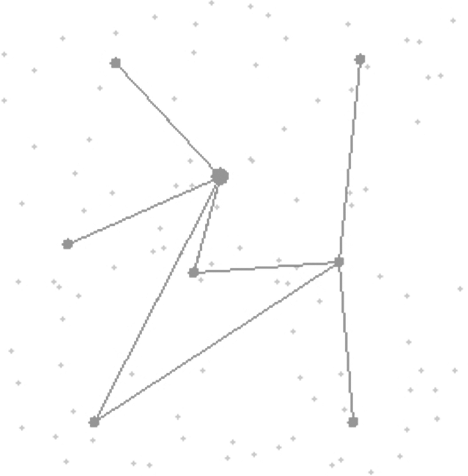
It is clear that the first part of (11) and (12) are energy due to distances (Edd). It is the only component that can be optimized independent from parameters related to the microcontroller and the supply voltage used. Consequently, Edd was used as the energy loss based on the distance for formation of clusters. Fig. 1 depicts the parameters we are minimizing in the energy model


Energy model based on the distance
Energy based Growing Self-Organizing Map (E-GSOM)
The Growing Self-Organizing Map (GSOM) is one of the variants of the Self-Organizing Map (SOM) that has the capability to achieve adaptive shape and size [13]. GSOM can be used as an automatic cluster detection tool without the knowledge of the number of clusters. Thus, it is also considered as an undirected technique with robust performance and diverse application. It has been applied to textual document data mining [14], classification [15], and clustering [16]. GSOM has the same topology structure and weight adaptation rules as the SOM and it can grow under the control of Spread Factor provided by the user, which the SOM cannot.
We propose in this paper an extended version of GSOM based on energy loss described in Eq. (13). The topology formed by an extended algorithm called energy based GSOM (E-GSOM) would be a hierarchical structure with cluster-heads at level-1 and sensing nodes at level-0. The E-GSOM has three basic training phases, namely Growing Phase, Ordering Phase, and Tuning Phase. Apart from the growing phase, other phases function similar to SOM [17]. However, since the feature map is also partially ordered in the growing phase, the training duration for the remaining two phases are considerably shorter than in SOM. The growing phase of the E-GSOM is described in a pseudo-code below:
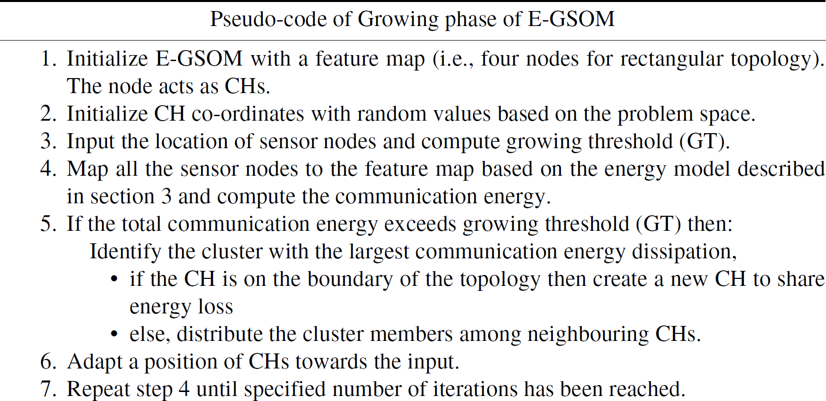
In the growing phase, the initial E-GSOM shown in Fig. 2 (arrows indicate the growing directions) starts mapping an input data to an appropriate map size and shape. The final map size (i.e., the number of cluster-heads) is determined from the spread factor (SF), which is user defined. The spread factor controls the spread of the map or the number of clusters. The Growing Threshold (GT) is defined in (14), where D is the dimension of the input space. In our case D = 2, because we have considered 2-D space. GT determines when to add more CH to the problem space. In Fig. 3, the boundary node is growing to create two new cluster-heads, thus distributing the energy dissipation to all the feature map nodes. The smoothing phase of E-GSOM is similar to Kohonen's SOM algorithm [17], it fine tunes the topology map outputted from the growing phase of E-GSOM algorithm without altering the size of the map:


E-GSOM Initialization.

New node generation from the boundary node.
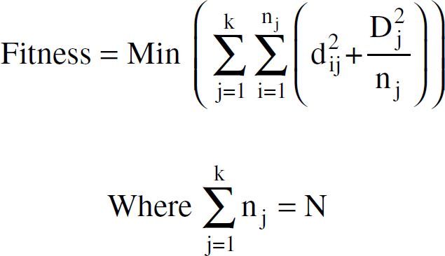
Evolutionary algorithms can be applied to find the solutions to NP-hard problem such as clustering, as they allow a wide search in the problem space. Genetic algorithm (GA) [18] and particle swarm optimization (PSO) [19] are few of the widely used evolutionary techniques. However, the main advantage of using an evolutionary algorithm in our problem is the ability to define a fitness function corresponding to the energy usage. In Both GA and PSO, the energy model (13) influences the cluster formation. Thus for given “K” clusters and “N” number of sensor nodes, the cluster is formed and CHs are identified by minimizing Eq. (15).
Genetic Algorithm (GA) is a searching technique that emulates the natural biological evolution. GA has been used for the clustering of data points [20] [21]. GA operates on a population of potential solutions applying the principle of survival of the fittest to produce better approximations to a solution. GA starts with a set of solutions called chromosomes. In our problem the co-ordinates of the CH are the chromosomes. The set of chromosomes are called the population. In each generation:
The population is evaluated with Eq. (15) in the problem domain. The chromosome with the best results will be selected for the next generation. The chromosomes are breed by using crossover and mutation The offspring are evaluated in the problem domain. The best possible offspring is reinserted into the population.
This process continues for a certain number of iterations or generations.
PSO based clustering approach
Particle Swarm Optimization is an evolutionary computing technique based on the principle of bird flocking. In PSO, a set of potential cluster-heads is called a particle and is initialized randomly. Each particle will have a fitness value, which will be evaluated by the fitness function (15) to be optimized in each generation. Each particle knows its best position, pbest, and the best position so far among the entire group of particles, gbest. The particle will have velocities, which direct the flying of the particle. In each generation, the velocity and the position of the particle will be updated. The equation for the velocity and positions are given below in (16) and (17) respectively.
Vik velocity of particle i at iteration k Vik+1 velocity of particle i at iteration k + 1 W inertia weight c1, c2 acceleration coefficients rand random number between 0 and 1 xik current position of particle i at iteration k pbesti pbest of particle i gbest gbest of the group xk+1 position of the particle at iteration k + 1

We have set the inertia weight to [0.5 + rand/2] as proposed in [22] and the Time-Varying Acceleration Coefficients (TVAC) technique proposed in [23] is used to vary the value of acceleration coefficients c1 and c2. This version of PSO called PSO-TVAC used for our simulation.
We further used general purpose clustering algorithms like K-mean, fuzzy-C-mean, and subtractive clustering to form the sensor clusters using the coordinates of the sensor locations. In these algorithms, energy minimization has not been exploited as the criterion for cluster formation. However, the quality of the clusters formed is evaluated by transmitting 512 bits of data from all nodes to the base station.
In k-mean clustering the N number of nodes are divided into K clusters, minimizing some metrics relative to the cluster center. Various metrics can be minimized such as,
distance from the cluster center to the sensor node total distance between all the nodes and their respective CHs.
The clusters are defined by their CHs Ci. For a given set of sensor nodes, the goal is to partition the nodes in set Si to minimize the euclidean distance between the set of sensor nodes Ni and the cluster-heads Ci:

Xn is the current pattern
Whereas the cluster-head Ci is defined by

K-means clustering requires a batch operation where the samples are moved from cluster to cluster to minimize (18) [24]. The advantage of using the k-mean clustering is the consistency of result if we know the number of clusters K. The algorithm normally converges quickly. The disadvantages are:
the algorithm may not reach both global and local optima we must specify K before the start of the algorithm.
In Fuzzy-c-mean (FCM) based algorithm, each node belongs to a cluster to some degree that is specified by a membership grade [25]. The FCM algorithm uses reciprocal distance to compute the fuzzy weights. When a node is of equal distance from two cluster centers, it gives the same weight on both the clusters independent from the distribution of the clusters.
Subtractive clustering is a useful algorithm if we are not certain about the number of clusters. It assumes each node as a potential cluster center and calculates the measure of the likelihood that each node defines the cluster center, based on the density of surrounding nodes [26].
The clustering algorithms explained in this section are categorized into:
customized clustering algorithms generic clustering algorithms.
In customized clustering algorithms, the algorithms which use energy model for clustering are included. These are E-GSOM, PSO-TVAC, and GA algorithms. In generic clustering algorithms, the algorithms that do not use energy model for clustering such as GSOM, K-Mean, FCM, and subtractive clustering are included.
From Eq. (13) we can conclude that reducing the communication distance in a network will reduce the energy dissipation in a network. To evaluate the goodness of our algorithm, we calculate the overall communication energy dissipated to transmit 512 bits of data from all the sensor nodes to the remote base station. The size of the data is for experimental reason and it can be altered. The following is the communication energy spent to transmit 512 bits of data from all the sensor nodes to base station:
Energy to transmit 512 bits of data from each sensor node. Eq. (2) is used to compute transmission energy. Energy in CH to receive all the data form cluster members. Eq. (4) is used to calculate receiving energy in CH. Energy in CH to aggregate data. The data aggregation model used in n: 1, i.e., for every n data packet received by CH only 1 packet must be sent to the base station. Typically n is the number of nodes in the clusters. The computation energy used for aggregation is 5 nJ/bit/signal [6]. Transmission energy in CH to transmit aggregated data to base station.
For our experiments, we used two different sensor networks (SN1 and SN2) both containing 100 nodes that are distributed in a 2-Dimensional problem space (0:100, 0:100). The base station is located at (50,175). We applied all the algorithms for both the set of nodes to form 4, 6, 8, and 12 clusters. The quality of the cluster is evaluated by transmitting 512 bits of data from all sensor nodes to the base station.
In K-mean based clustering, we randomly place the cluster-head and each cluster-head will form a cluster based on the Euclidian Distance Measure. The algorithm will be terminated when there is no significant improvement in the position of the cluster-head. The number of clusters “K” is pre-defined in the algorithm.
In FCM based clustering, the cluster-heads are randomly distributed and each node will be assigned a membership grade for each cluster-head. Iteratively, the cluster-head will move to the right direction improving the membership grade.
In Subtractive Algorithm Based Clustering, each node must be set at a influence range. Here, each node is considered as a potential cluster-head. The algorithm calculates the measure of the likelihood that each node would define a cluster. The node with highest surrounding density is selected as a cluster-head. For comparison with other algorithms, we experimentally set an influence range appropriately to obtain 4,6,8, and 12 clusters.
In the GSOM based clustering algorithm, we have used rectangular topology for the initial feature map. Each node in a feature map represented a cluster-head in a sensor network. Initialization starts with four nodes in a feature map because of rectangular topology. Sensor nodes placed in the problem space are mapped to the feature map based on the smallest euclidean distance. The number of nodes in a feature map grows based on the growing threshold, which is influenced by the spread factor. When the feature map stops growing, the feature map is calibrated in the smoothing phase. If there is no sensor node at the optimal cluster center, the sensor closest to it will be assigned a CH. We obtain required number of clusters by tuning the value of the spread factor of the feature map. In all the above algorithms, the energy model doesn't influence cluster formation. However, energy consumption to transmit 512 bits of data from each node to the base station through cluster-heads is used to evaluate the goodness of the cluster formation.
In E-GSOM algorithm, the energy model discussed in section 3A. It influences the growth of the network feature map. In the growing phase, the energy consumption in the network is used as the criterion for the growth. At the end of each epoch the total energy consumption is calculated and compared with the growing threshold. If the total energy in the network is greater than the growing threshold, the cluster with the highest energy consumption will grow. This method gives good results when the initial feature map has grown to contain a higher number of nodes from the starting position of four nodes.
In the GA based algorithm, we optimized the placement of cluster-heads (CH) in the 2-D space. We used a simple GA algorithm with single-point crossover and selection was based on a roulette wheel process. We used the co-ordinates of the cluster-heads (CH) as the chromosomes, and the fitness function as suggested in Eq. (15) is minimized.
The PSO-TVAC based algorithm we have proposed was also used to find the clusters and the corresponding cluster-heads. The particles were the co-ordinates of the potential CHs randomly generated. We used 30 particles for our experiments, and the maximum number of generations we were running was 1000. The maximum velocity of the particle was set to the length of the side of the problem space. If the particle converges more at the boundary of the problem space or go beyond the problem space, we would move the particle back to the problem space randomly. We minimize Eq. (15). PSO-TVAC converges quickly when compared to the other evolutionary techniques. This is mainly because of the velocity factor of results from table 1 to 4 are for SN1 nodes and from table 5 to 8 are for SN2 nodes.
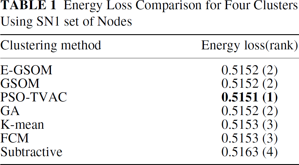
Energy Loss Comparison for Four Clusters Using SN1 set of Nodes
Energy Loss Comparison for Four Clusters Using SN1 set of Nodes
Energy Loss Comparison for Six Clusters Using SN1 set of Nodes

Energy Loss Comparison for Eight Clusters Using SN1 set of Nodes

Energy Loss Comparison for Twelve Clusters Using SN1 set of Nodes

Energy Loss Comparison for Four Clusters Using SN2 set of Nodes

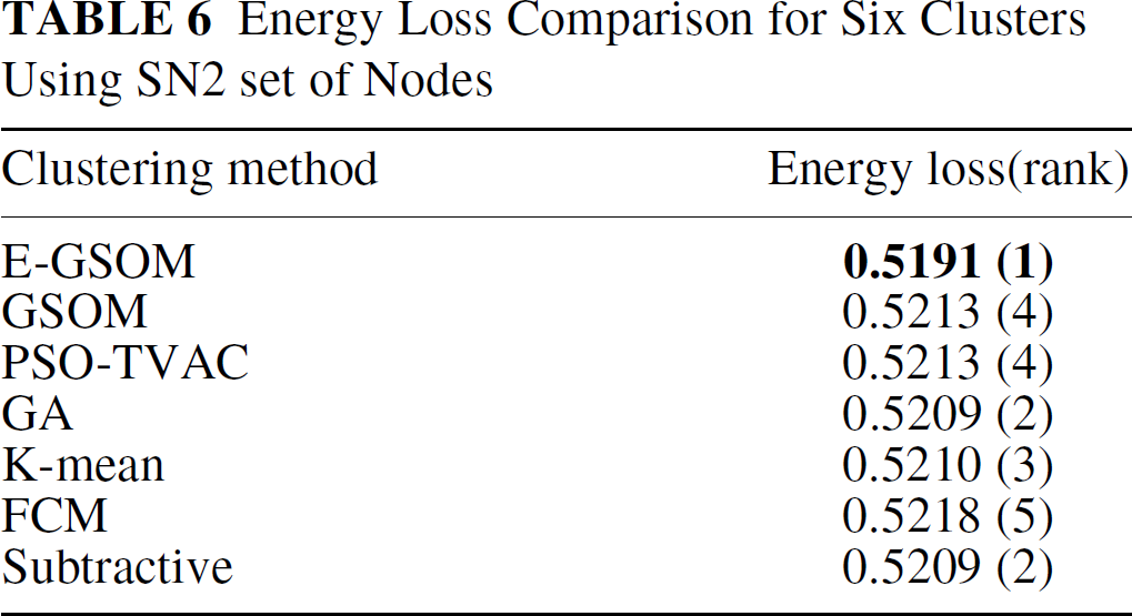
Energy Loss Comparison for Six Clusters Using SN2 set of Nodes
Energy Loss Comparison for Eight Clusters Using SN2 set of Nodes

Energy Loss Comparison for Twelve Clusters Using SN2 set of Nodes

We allowed GSOM and E-GSOM to grow from 4 to 6, 8, and 12 clusters by changing the spread factor. For four clusters, the GSOM and E-GSOM algorithms give similar to SOM as there is growing phase used. However, when the feature map grows, E-GSOM always gives a better result than GSOM. This is due to the influence of the energy model used in the growing phase. From the experimental results in Table 2, 3, 4, 6, 7 and 8 we can conclude that E-GSOM clustering technique was the best four out of six times. The only time it doesn't perform well is when the map is not growing, i.e., when the number of clusters is four and the results are given in Table 1 and 5. A positive feature of E-GSOM and GSOM is the consistency of its clusters and the energy loss observed in multiple runs. Using GSOM and E-GSOM we could improve the performance as well as the cluster formation further by tuning the spread factor and by increasing the number of epochs. All the GSOM and E-GSOM results presented in this paper are simulated for certain number of epochs (five for our simulation). Furthermore, the number of clusters in GSOM and E-GSOM is determined by simply controlling the spread factor, where as in other cluster algorithms used except subtractive clustering the number of clusters has to be predetermined. The better results obtained with E-GSOM are due to various reasons. Firstly, the final weight (co-ordinate) vectors define prototypes of the cluster-heads reflects the density distribution. In addition to this advantage, E-GSOM will grow based on our proposed energy model. This helps in the algorithm to grow with less energy loss than GSOM. Fig. 4 and 5 shows the cluster formation and CH representation in E-GSOM and GSOM for six and eight clusters respectively. The topology used in both cases is rectangular. In Fig. 5, the CHs are placed more close to high density nodes when compared to Fig. 4. This is mainly because only intra-cluster distance influences the cluster formation in GSOM where as in E-GSOM the distance to the remote base station and the number of nodes in a cluster would also influence the cluster formation.

Cluster formation using F-GSOM with rectangular topology. The small dots are sensor nodes and the big dots are cluster head (CH)
Eight cluster formation using GSOM with rectangular topology. The small dots are sensor nodes and the big dots are cluster-heads (CII)
GA algorithm gave consistently good results and was always in top three positions. However, it was the top performer only once. The algorithm can be further improved by incorporating multiple crossover and better selection method to the GA algorithm.
The main disadvantage of the PSO-TVAC is the inconsistency of the result. Therefore, it is always advisable to apply the simulation few times and average the results. We applied the algorithm ten times to minimize the inconsistency of the result. PSO-TVAC gave best results in Table 1 and 2. Overall, the results are very close to GA if not better. This is not surprising given the stochastic nature of the algorithm.
Among conventional clustering algorithms, K-mean was better most of the time. When the number of clusters are small, the algorithms are competitive.
Here is the summary of the analysis of all the results from both SN1 and SN2:
With four clusters, all algorithms gave a similar results. overall, E-GSOM gave the best results and GA and PSO-TVAC were second. The outcome is on the expected lines because all the algorithms are customized clustering algorithms. Among generic clustering algorithms, if we consider higher order clusters, GSOM performed better. With four clusters, K-Mean has performed better.
In this paper, we described the energy model to minimize the energy dissipation based on the communication distance in a sensor network. We proposed the extension of GSOM called E-GSOM to cluster sensor nodes in a sensor network. We have simulated two evolutionary computing techniques including an extension to PSO for cluster formation. However, E-GSOM provides the best performance, in addition it is the fastest algorithm among the seven algorithms tested.
It is intended to incorporate the energy as E-GSOM's growing threshold instead of spread factor, such that we can restrict the size of the cluster and the number of clusters based on the energy available in the network. This will also help to attach new nodes to the network when energy loss exceeds the specified limit. The incorporated constraint should allow more rapid flexibility in handling the overall network. We would like to improve the energy model by considering the higher order radio model. We intended to work on the application with large problem space. For these kinds of applications, a node transmission range cannot cover the entire network. Thus, we are working on the clustering algorithm with transmission range restriction.