Data Capacity Improvement of Wireless Sensor Networks Using Non-Uniform Sensor Distribution

Abstract

Energy conservation is an important design consideration for battery powered wireless sensor networks (WSNET). Energy constraint in WSNETs limits the total amount of sensed data (data capacity) received by sinks. In the commonly used static model of sensor networks with uniformly distributed homogenous sensors with a stationary sink, sensors close to the sink drain their energy much faster than sensors far away from the sink due to the unevenly distributed forwarding workloads among sensors. A major issue, which has not been adequately addressed so far, is the question of how sensor deployment governs the data capacity, and how to improve data capacity of WSNETs. In our previous work, we provided a simple analytical model to address this issue for one specific type of WSNETs. In this paper, we extend our previous work to address this issue for general WSNETs. In the extended static models, for large networks, we find that after the lifetime of a sensor network is over, there is a great amount of energy left unused, which can be up to 90% of the total initial energy. Thus, the static models with uniformly distributed homogenous sensors cannot effectively utilize their energy. This energy waste implies that the potential data capacity is much larger than the capacity achieved in these static models. To increase the total data capacity, we propose a non-uniform sensor distribution strategy. Simulation results show that, for large, dense WSNETs, the non-uniform sensor distribution strategy can increase the total data capacity by an order of magnitude.

I. Introduction

A wireless sensor network (WSNET) consists of a set of micro sensors deployed within a fixed area. The sensors sense a specific phenomenon in the environment and route the sensed data to a relatively small number of central processing nodes, called sinks. Unlike a mobile ad hoc network (MANET) where bandwidth efficiency and throughput are two important metrics, energy conservation is an important design consideration for WSNETs since sensors are constrained by battery power.

A sensor in a WSNET plays two roles: sending its own sensed data and forwarding sensed data of other sensors to a sink. If the sensed phenomenon is uniformly distributed (which means that all sensors have the same amount of data to report) and all sensor readings generate non-aggregative data, the energy consumed for the former role of each sensor is approximately identical. However, the energy consumption for the latter role is not. One observation is that the closer a sensor is to the sink, the higher the forwarding workload. In energy constrained WSNETs with stationary sensors and a sink, neighbor sensors of the sink deplete their energy faster than other sensors. Since the sink can only receive sensed data from its neighbor sensors, the network data capacity, which is defined as the total amount of data received by the sink, is bounded by the total initial energy of neighbors of the sink. Intuitively, there is an unknown amount of energy left unused in sensors far away from the sink after the lifetime of the network is over. Here lifetime of the network can be defined as the time lasted when a certain percentage of sensors are disconnected from the sink. This percentage is varied in different application environments. Since this unknown amount of unused energy indicates the further improvement space of the data capacity of a WSNET, it is useful to find it.

Similar to mobile ad-hoc networks (MANETs), researchers have focused on the MAC and network layer protocols for WSNETs [1, 3, 4, 5, 6, 7, 8, 17]. Data aggregation techniques also have been studied in references [3, 8, 9]. In fact, all of these works focus on increasing energy efficiency of a WSNET, which is represented by the average energy required to transmit a unit of sensed data to a sink. However, in the commonly used general static models of WSNETs, in which homogenous sensors are uniformly distributed in the sensed area with static sinks, energy efficiency is not the most important factor in WSNET operation. Instead, we will show in this paper that careful deployment of sensors and sinks has a positive impact on data capacity. A few techniques for making sensor networks energy efficient to improve their data capacity have been reviewed in Section II.

In our previous work [18], we have addressed energy utilization in the Single Static sink Edge Placement model (SSEP), in which homogenous sensors are uniformly distributed in the network area with a single static sink located on an edge of the network area. In the SSEP model, energy of sensors is not efficiently utilized. To improve energy utilization, two strategies have been proposed as follows. First, we make the sink mobile so that it does not have the same bottleneck as a static sink. Second, we let the sensors be uniformly distributed, but the sensors themselves are non-homogenous in terms of their initial energy.

In this paper, we extend the SSEP model to a set of models, where random placement of the sink and multiple static sinks are supported. These models are evaluated in terms of two performance metrics: total network data capacity and unused energy ratio. Unlike the transport capacity discussed in [10, 11], network data capacity of a WSNET is the total amount of sensed data received by the sinks. Since a model with lower unused energy ratio does not mean that it has higher data capacity than another model, we use the total network data capacity as the primary performance metric and unused energy ratio as the secondary. The contributions of this paper are as follows.

We give a mathematical model for data capacity and energy utilization in a WSNET with one static sink. The sink can be located at different positions in the network area, such as on an edge, at a corner, and in the center. To compute energy utilization, we assume to know the energy needed to transmit a unit of sensed data to the sink, and give a model of the average hop length of shortest-hop paths from all sensors to the sink. From the established model, we observed that the energy as high as 90% is left unused after the lifetime of the network is over, and the total data capacity achieved is very small compared to the maximum potential data capacity.

We give a mathematical model of data capacity and energy utilization for a WSNET with multiple sinks deployed on an edge. We observed that a great amount of energy is still wasted. These results suggest that the static models are not a proper choice for large-scale sensor networks.

The main reasons for the low energy utilization are the uniform energy level of sensors and the stationary sinks. To make the best use of energy resources in sensors, we propose a non-uniform sensor distribution strategy and a routing protocol. Simulation study shows that it can improve the total data capacity by an order of magnitude compared to the capacity achieved in the static sink model for large WSNETs.

For the models in this paper, without loss of generality, some basic assumptions are made as follows. The network area is a fixed W x H rectangular area with width W and height H. N sensors are randomly positioned according to Poisson distribution with density λ sensors per unit area. All sensors are homogeneous with the same amount of initial energy P_s and transmission radii r_s. Each sensor consumes e_s quantity of energy to transmit one bit of sensed data to its neighbors. The communication link (connection) between two sensors is symmetric. The locations of sensors and sinks remain unchanged. Sinks have unlimited energy and the same range r_s as the sensors. The energy required to transmit data is far more than the energy consumed by CPU processing, sensing, and data receptions. Thus, only the power consumption of data transmissions is considered. The sensed phenomenon is uniformly distributed over time. All sensor readings generate non-aggregative data. Two nodes (sensor or sink) are said to be neighbors if they are within the transmission range of each other. The average degree (denoted by g) of a node is defined as the average number of neighbors for all nodes in the network. From [2], when N nodes are randomly distributed over a unit area, to ensure a certain probability of node connectivity, the asymptotic lower bound of the average degree is Ω(logN). To deploy a sensor network with hundreds of nodes connected with high probability, say, 0.95, the average degree is at least 4 [12, 13, 14]. In this paper, the required average degree is greater than or equal to 5 in all sample networks to ensure more than 95% of total nodes are connected together.

The rest of the paper has been organized as follows. In Section II, we review the related works. In Section III, some important properties of the shortest hop paths are discussed and the performance of WSNET in the single static sink model, which is the foundation of subsequent models, is analyzed. We extend our analysis of the single static sink model to multiple sinks located on an edge in Section IV. A non-uniform energy distribution model and its related routing protocol are given in Section V. Finally, some concluding remarks are given in Section VI.

II. Related Works

A. Literature Review

Electrical energy is a critical resource in WSNETs. In many outdoor applications, sensors may be powered by batteries. Depending on the network area to be sensed, the batteries of the sensors may not be replenished. Hence, it is important to efficiently consume energy with the goal of maximizing the network life time for a given amount of total initial energy. If care is not taken, sensors close to the sink will run out of energy much earlier than sensors far away from the sink, causing the network to die even though a majority of the sensors are still operational. Also, it is desirable to operate the network such that all the nodes are left with zero amount of energy when the network dies. Intuitively, energy efficiency can be achieved in several ways, such as

(i)

having sensors adjust their transmitting power to reach a suitable next-hop neighbor with minimal energy consumption,

(ii)

having sensors forward fewer average number of messages on behalf of other sensors, and

(iii)

giving sensors close to a sink more initial energy than sensors farther away.

The power required to transmit data between two nodes can be modeled as (c + d^α), where d is the distance between the two nodes, α a constant (2 ≤ α ≤ 6), and c is another constant [19]. Hence, in energy constrained WSNETs, sensors far away from the sink may not directly send data to the sink. Multi-hop communication is one choice to reduce the transmission cost involved in long distance communication. In multi-hop communication, neighbor sensors of the sink deplete their energy faster than the other sensors. After the lifetime of the network is over, there is a great amount of energy left unused. A power-cost localized routing algorithm has been proposed in [19] to overcome the non-uniform energy drainage problem and to minimize the total energy needed. In this algorithm, sensors are assumed to be able to adjust their transmission power to a level good enough to reach a next hop neighbor. A power-cost metric based on the lifetime of both nodes and distance-based power metric has been defined and used to compute the shortest weight path by applying Dijkstra's algorithm.

In [20], the authors have proposed a clustered network model by using sensors with adjustable transmission power. Two types of nodes are used in their model: normal sensors and cluster headers (CH). The network is partitioned into multiple clusters and each cluster has a CH. A CH aggregates data received from sensors within its cluster and then directly sends the aggregated data to the sink. Normal sensors can send sensed data to CHs by using two modes: single-hop and multi-hop. In the single-hop mode, all sensors in a cluster directly send data to the CH. According to the assumption of uniformly distributed sensors with identical initial energy and the capability of adjustable transmission power, the sensors far away from the CH deplete their energy faster than the sensors close to the CH. In the multi-hop mode, each cluster is partitioned into a set of concentric rings, and sensors in one ring always forward data to sensors in the next ring closer to the CH. In this mode, sensors in the inner-most ring exhaust their energy faster than sensors far away from the CH. To overcome the non-uniform energy drainage problem in these two modes, a hybrid mode is proposed. In this mode, sensors use the single-hop mode and multi-hop mode interchangeably.

The works reported in [19] and [20] use transmission power adjustable sensors. If all sensors have a fixed identical transmission range, those two techniques cannot be applied. In [18], we distribute energy among sensors in a multi-hop network in a non-uniform manner so that all the sensors deplete their energy almost at the same time. In this paper, under the assumption that all sensors have an identical transmission range, we propose a solution to overcome the non-uniform energy drainage problem by using non-uniformly distributed homogenous sensors. We believe that energy efficiency techniques, such as sensor capability to transmit at variable power [19], using a combination of single-hop and multiple-hop communication [20], non-uniform energy distribution among sensors [18], and non-uniform sensor distribution (in this paper), give network designers an array of alternative choices. What technique gives the best network lifetime with a given amount of initial energy is out of scope of this paper.

B. Progress, Max-progress and Max-progress Paths

In this sub-section, we briefly review several important concepts: progress, maximum one-hop progress, and max-progress path [22, 24]. For a more detailed background of these concepts, readers may refer to [23]. There we give approximate estimations for maximum one-hop progress and max-progress paths. Meanwhile, some important equations are listed. These concepts, their estimations, and equations will be used in this paper.

The concept of progress is mainly used in geographical routing strategies [14, 15, 22, 24]. Let d(PQ) denote the distance from P (sensor) to Q (sink) in Fig. 1. If P forwards a packet to a neighbor P′, the one-hop progress (denoted by z) from P to P′ is defined as z = d(PQ) - d(P′Q). For any sensor P, if P chooses a neighbor sensor, to which P has the maximum value of one-hop progress among all its neighbors, as its next forwarding node, then this one-hop progress is called maximum one-hop progress (denoted by Z) of P. A forwarding path established by a set of sensors using maximum one-hop progress to forward data is called a max-progress path.

Figure 1

One-hop Progress from P to Q.

In a WSNET with randomly distributed sensors, the average maximum one-hop progress (denoted by Z̅ (1)) is a function of average degree g, distance d, and radius r_s. For randomly distributed sensors, we have

$$g=\lambda \pi r_s^2$$

(1)

Two solutions of Z̅ are presented in [14, 15]. However, the solutions are too complex to be applied into our model. According to [14], if the ratio of r_s and d is sufficiently large, Z̅ is a function of the average degree g only and the influence of d and r_s is not significant. Thus, we use the approximation in [18] as follows:

$$\bar{\mathrm{Z}}\approx 1-e^{-\frac{1}{2}\sqrt{g}}-0.07-0.09e^{(5-g{)}^{\frac{1}{3}}}$$

(2)

where Z̅ is normalized to transmission radius r_s (r_s is treated as unity) and g ≥ 5. From the simulation results shown in [18], the computed values of Z̅ from (2) closely match with the simulated values of Z̅ with g ranging from 5 to 80 and the ratio of d/r_s ranging from 5 to 60. The more detailed results can be found in [18].

Each max-progress path has a certain number of hops. Next, we will review how to estimate the average hop number of all max-progress paths to the sink. Since the distance from a sensor to the sink is known and each transmission makes r_sZ̅ progress on an average along a max-progress path, the hops for this path can be computed. Therefore, to compute the average hop length, the average distance from all sensors to the sink needs to be computed. Due to the uniformly distributed phenomenon and sensors in the sensed area, finding the average distance is equivalent to finding the average distance from all points in the network area to the sink. Assume that the sink is located at (x_c, y_c) in a W × H rectangular network area and let d̅ (1) denote the avserage distance. According to [18], the average distance (denoted by d̅(W, H, x_c, y_c)) is given as follows.

$$\begin{array}{rl}\bar{d}(W,H,x_c,y_c)=\frac{1}{WH}& \hspace{0.5em}(V(x_c,y_c)+V(y_c,x_c)+V(W-x_c,y_c)+V(y_c,W-x_c)+\\ & V(x_c,H-y_c)+V(H-y_c,x_c)+V(W-x_c,H-y_c)\\ & \hspace{0.5em}+V(H-y_c,W-x_c)),\end{array}$$

(3)

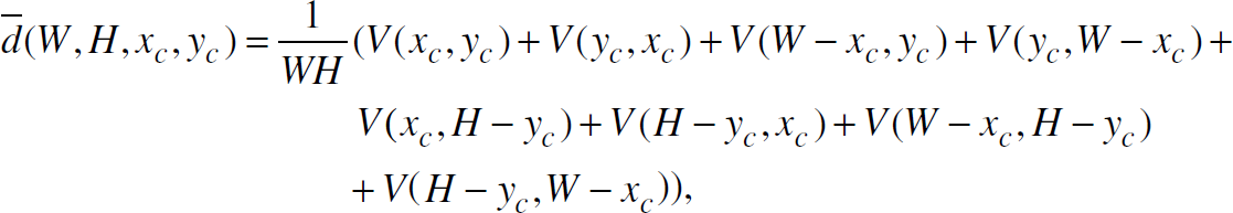
where the volume function V(x, y) is:

$$V(x,y)=\{\begin{array}{l}0ifx=0\mathrm{\hspace{0.5em}\hspace{0.5em}}ory=0\\ \frac{x^3}{6}(\text{ln}(y+\sqrt{x^2+y^2}-\text{ln}(x)+\frac{y}{x^2}\sqrt{x^2+y^2})otherwise\end{array}$$

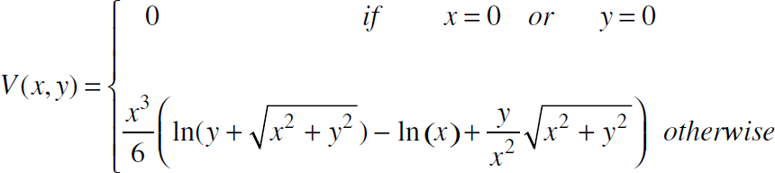
Therefore, from (2) and (3), the approximated average hop length h̅ for all maxprogress paths is:

$$\bar{h}\approx \frac{\bar{d}}{r_s\bar{Z}}=\frac{\bar{d}}{r_s(1-e^{-\frac{1}{2}\sqrt{g}}-0.07-0.09e^{(5-g{)}^{\frac{1}{3}}})}$$

(4)

III. Single Static Sink Models

In this section, we consider three static models of WSNETs with a single stationary sink, and analyze its data capacity and energy utilization. The only difference among the three models is the location of the sink. If the sink is located on an edge of the rectangular network area, the model is referred to as the Single Static sink Edge Placement (SSEP) model. The second model is referred to as Single Static sink cOrner Placement (SSOP) model, in which the sink is located at one corner. Similarly, the third model is referred to as the Single Static sink Center Placement (SSCP) model, in which the sink is placed in the center. We refer to a sensor network in the three models as an SSEP, SSOP, and SSCP network, respectively.

A. Methedologies

To compute energy utilization of a WSNET, we need to know the total amount of energy consumed to transmit all sensed data. For a given data capacity Ψ in a WSNET, if we know the average number of transmissions (or hops) required for relaying a unit amount of sensed data to the sink, we can obtain the total amount of energy consumed to transmit these Ψ bits of sensed data, and the network energy utilization can be obtained. The average number of hops required for relaying sensed data to the sink depends on the routing algorithm used. Since the transmission cost is minimized if data is relayed through shortest-hop paths to the sink, the energy utilization in this paper is computed based on shortest path forwarding. Direct computation of the average hop length of all shortest paths from all sensors to the sink is not straightforward. Instead, we will show that the average hop length of the shortest paths in a network can be approximated by the average length of all max-progress paths (Section II.B).

The practical meaning of the average maximum one-hop progress is illustrated in Fig. 2, in which sensors are randomly deployed in a rectangular area. The dark points in Fig. 2 denote sensors with an odd number of shortest hops to the sink and the gray points denote sensors with an even numbers of shortest hops to the sink. The odd and even hop sensors are interleaved with each other. The smallest circle centered at the sink has the same radius as the transmission range r_s. All the other circles have the radius given by r_s + k Z̅ r_s, where k is a positive integer. Let V₁ denote the area enclosed by the smallest circle and V_k the area bounded by two adjacent circles with radii r_s + (k − 2) Z̅ r_s and r_s + (k − 1) Z̅ r_s, respectively, for k ≥ 2. Each V_k is called the k^thcritical region.

Figure 2

Distribution of Random Deployed Sensors.

From Fig. 2, we observe that almost all sensors with the same shortest hop distance k to the sink are located in the k^th critical region. This observation indicates that each forwarding from a sensor P in V_k along a shortest path delivers data to a sensor P′ in V_k−1 on an average. Hence, the average one-hop progress along the shortest paths is approximately equal to the average maximum one-hop progress estimated in (2). Another observation is that for all sensors which are k (k ≥ 2) hops away from the sink, the average distance from these sensors to the sink is approximately equal to.

$$r_s+(k-1)\bar{Z}{r}_s-0.5\bar{Z}{r}_s=r_s+(k-1.5)\bar{Z}{r}_s$$

(5)

Using simulation studies, we verify the two claims related to the shortest paths as follows.

• (i)

The average hop length of the shortest paths can be approximated by the average length of max-progress paths given in (4).

(ii)

The average distance from all sensors with the same shortest hop to the sink can be computed by (5).

For each simulation, we randomly deploy a fixed number of sensors in a W × H network area. The sink is always located at the middle of one width edge. Since we know the shortest hop count of each sensor to the sink, we can compute the average hop length for all sensors. Meanwhile, we compute the average distance from all sensors with the same hop count to the sink and record these average distances for most of possible hops. Then these two sets of simulated results are compared with the results predicted using (4) and (5), respectively.

Figure 3 compares the simulated average hop length of shortest paths and the predicted average hop length of max-progress paths for a square network area. In this figure, the x-axis denotes the ratio of W and the transmission (TX) radius r_s. Figure 4 shows the comparison results for the second claim. In Fig. 4, the x-axis denotes the shortest hop count to the sink. Then the average distance from all sensors with this hop is computed. In Figs. 3 and 4, the data series are labeled in the format of either P-g or S-g, where g = 8, 14, or 20. In these labels, P denotes the Predicted result, S the Simulated result, and g the average degree of the given WSNET. All data points on all curves are computed by taking the average of 50 samples. From Figs. 3 and 4, we observe that the predicted results closely match the simulated results. For different network configurations, according to the results not shown here, the two claims hold with high accuracy. Therefore, the properties of shortest paths can be approximated by the properties of max-progress paths in WSNETs. The comparison results also indicate that the max-progress paths perform almost, equally well as shortest hop paths. Thus, a routing algorithm based on max-progress paths could be a good candidate in WSNETs.

Figure 3

Results of Average Hop Length (W = H).

Figure 4

Results of Average Hop Length (W = H).

B. Network Data Capacity in the SSEP Mode

In the SSEP model shown in Fig. 5, we assume that the sink node is located at coordinate (x_c, 0) and it is at least r_s distance away from the corners of the network area. Each SSEP network is determined by six parameters: the area width W, height H, average degree g, transmission radius r_s, and location of the sink (x_c, y_c), where y_c = 0.

Figure 5

Illustration of an SSEP Network.

The total network data capacity $\bar{\mathrm{\Psi }}$ of an SSEP WSNET is defined as the total sensed data received by the sink (not including other data such as routing overhead). Let V₁ denote the first critical region defined in Fig. 2. It may be noted that V₁ contains an average of g/2 sensors. If all sensors in V₁ deplete their energy, the sink is disconnected to the network. Since the average total initial energy available in V₁ is gP_s/2 and transmission of one bit of data to the sink consumes e_s amount of energy, the total network data capacity $\bar{\mathrm{\Psi }}$ is expressed as follows.

$$\bar{\mathrm{\Psi }}=\frac{1}{2}\lambda \pi {r_s}^2\frac{P_s}{e_s}$$

(6)

Ψ can be achieved in an ideal situation where there is no routing overhead, no collision at the MAC level, and the energy consumed for sensing and computation are negligible compared to data transmissions.

C. Energy Utilization and Unused Energy Ratio in the SSEP Model

The energy utilization of an SSEP network is measured by the unused energy ratio μ, which is defined as the ratio of the remaining energy available in the network after all neighbors of the sink deplete their energy and the total initial energy. The total initial energy of an SSEP network is NP_s, where N is the total number of sensors and P_s is the initial energy in each sensor. From (6), in an ideal condition, $\bar{\mathrm{\Psi }}$ bits of data can be sent to the sink. According to the discussion in Section II and (4), each data bit in $\bar{\mathrm{\Psi }}$ should traverse h̅hops on an average to the sink, thus each data bit consumes h̅e_s amount of energy on an average. The total energy consumed to transmit $\bar{\mathrm{\Psi }}\text{bits}$ is $\bar{h}\hspace{0.17em}{e}_s\bar{\mathrm{\Psi }}$ . Therefore, the unused energy ratio μ is expressed as follows.

$$\mu =1-\frac{\bar{h}{e}_s\overline{Psi}}{N{P}_s}=1-\frac{\bar{h}\pi {r_s}^2}{2WH}$$

(7)

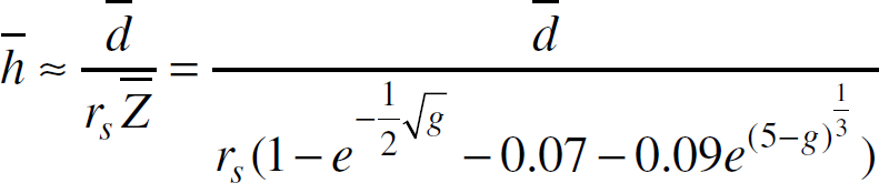
Figure 6 shows the result computed from (7) for networks with W = H. In this figure, the x-axis denotes the ratio of W and the transmission (TX) radius r_s, and the y-axis represents μ. Each curve is for a specific average degree g (5 ≤ g ≤ 30). The sink is located at coordinate (W/2, 0). Figure 6 illustrates the waste of energy of an SSEP network. In other simulation studies, approximately the same amount of energy is wasted for networks with different area shapes, such as W = 2H and W = H/2. The unused energy ratio μ is mainly determined by W/r_s, H and the average degree g. From this figure we conclude that a large amount of energy is wasted in an SSEP network. For example, when W/r_s = 15 and nodes have 10 neighbors on an average, about 90% of the total initial energy will be left unused. Hence, SSEP networks cannot utilize the total energy properly.

Figure 6

Predicted Unused Energy Ratio (W = H).

D. Simulation Results

We use a routing-level simulator to verify the unused energy ratio predicted by the model above and give the simulation results in Fig. 7. In the simulation, networks are configured using the SSEP model. N homogeneous sensors are randomly deployed in the network area. To make the results reliable, randomly generated sample networks have more than 90% of sensors initially connected to the sink. The sensed events are generated randomly with uniform distribution. The sensing range of each sensor is half of its transmission range. A simulation run terminates if 90% of the sensors are disconnected from the sink. If a sensor exhausts its energy or is disconnected from the sink, it stops functioning. The sink is located at point (W/2, 0). Figure 7 illustrates the simulated and predicted unused energy ratios for a network with a square area and average degree 16. Each simulated data point is calculated by taking the average of 40 runs. According to the figure shown above, the predicted data closely matches with the simulation results. By the simulation results, not shown here, with different configurations of network areas (such as W = 2H and W = H/2) and average degrees (5 ≤ g ≤ 30), the predicted data closely matches with the simulation results too. Therefore, for most of the commonly used ranges, the SSEP model can be used as a reference model for further analysis.

Figure 7

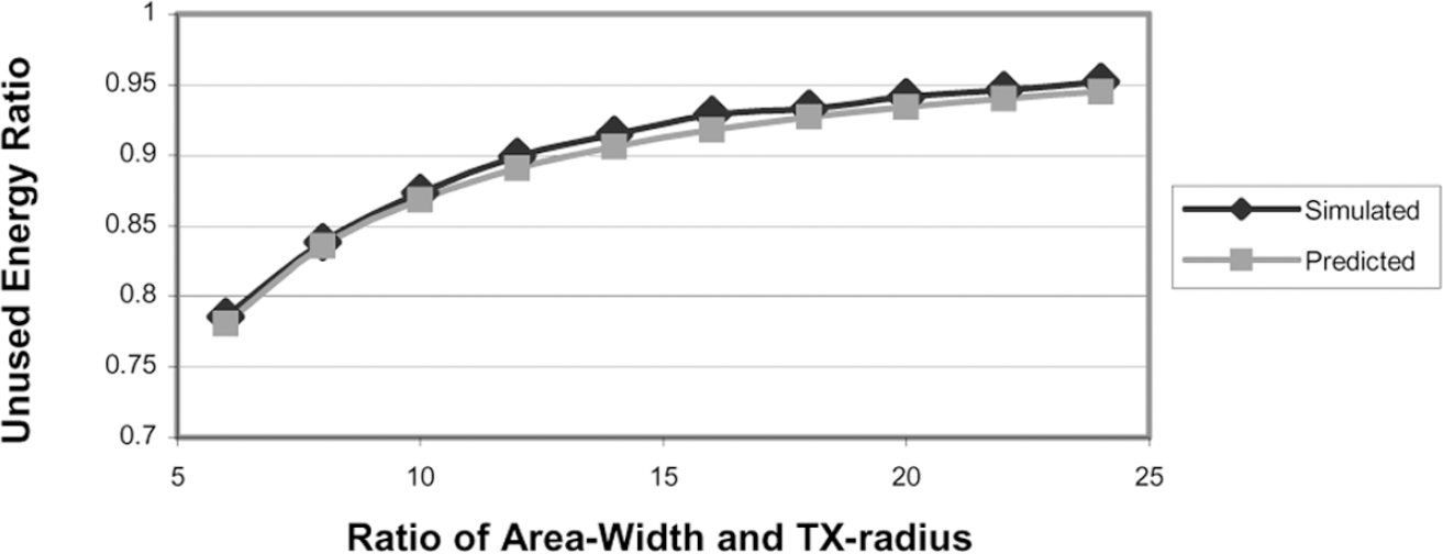
Simulated and Predicted Results (g = 16. W = H).

E. Single Static Sink Corner Placement (SSOP) Model

The SSOP model is a special case of the SSEP model, in which the sink is placed at a corner of the network area (Fig. 5). Obviously, the area of the first critical region in the SSOP model is half of the area of the first critical region in the SSEP model. Thus, the total data capacity in the SSOP model is half of the one in the SSEP model. Let ${\bar{\mathrm{\Psi }}}_{SSOP}$ and ${\bar{\mathrm{\Psi }}}_{SSEP}$ denote the data capacities in the SSOP and the SSEP model, respectively. We have

$${\bar{\mathrm{\Psi }}}_{SSOP}(W,H)={\bar{\mathrm{\Psi }}}_{SSEP}(W,H)/2$$

(8)

Equation (8) means that keeping other parameters unchanged, the average maximum data capacity in an SSOP network on W x H area is half of the capacity in an SSEP network on the same area. The unused energy ratio is

$${\mu }_{SSOP}=1-\frac{{\bar{h}}_{SSOP}{e}_s{\bar{\mathrm{\Psi }}}_{SSOP}}{N{P}_s}=1-\frac{{\bar{h}}_{SSOP}\pi {r_s}^2}{4WH}$$

(9)

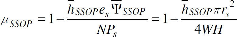
where h̅_SSOP is the average hop length of all shortest paths to the sink in an SSOP network.

F. Single Static Sink Center Placement Model

The center placement of the sink (SSCP) is shown in Fig. 8. Since the first critical region in the SSCP model is twice of the first critical region in the SSEP model, the maximum data capacity is doubled.

$${\bar{\mathrm{\Psi }}}_{SSCP}(W,H)=2{\bar{\mathrm{\Psi }}}_{SSEP}(W,H)$$

(10)

Figure 8

Center Placement Model of Sink Node.

As shown in Fig. 8, the entire W x H area can be partitioned into four sub-areas B₁, B₂, B₃ and B₄. For dense networks, data sensed by sensors in one sub-area generally will not be forwarded to the sink through the sensors in another sub-area. Only sensors very close to the boundary of two adjacent sub-areas may forward data to sensors in another sub-area. If the network area is sufficiently large, this boundary effect can be ignored. Therefore, an SSCP network is approximately equivalent to the four small networks, each of which is an SSOP network. So, we have

$${\mu }_{SSCP}(W,H)={\mu }_{SSOP}(W/2,H/2)$$

(11)

Figure 9 shows the unused energy ratio in three static models. These results state that no matter how a sink is placed in the network area, there is a great amount of energy left unused. Thus, the single static sink models with uniformly distributed sensors cannot effectively utilize their energy.

Figure 9

Unused Energy Ratio (W = H, g = 10).

IV. Model of Multiple Static Sinks

To improve data capacity and energy utilization, one strategy is to place multiple sinks in the network area. In this section, we will give a brief discussion of a Multiple Static sinks Edge Placement (MSEP) model, in which multiple sinks are allowed and all the sinks are located on the same edge.

For the MSEP model, there are three possible strategies for sensors to send sensed data to multiple sinks. The first strategy is to send sensed data to all the sinks, which is referred to as all sink notification. The second is to send sensed data to the closest sink and is referred to as closest sink notification. The third strategy is to send data to the interested sinks only, such as directed diffusion [1]. This strategy is referred to as interested sink notification. For the first and third notification strategies, even though the total data capacity increases compared with ${\bar{\mathrm{\Psi }}}_{SSEP}$ , the data contents are redundant. For the purpose of energy conservation, we prefer that sensors send data to the closest sinks and sinks exchange sensed data among themselves. Hence, we focus on the closest sink notification in this paper.

A. Finite Static Sink Edge Placement Model

First, we consider a WSNET in a special case of the MSEP model containing two sinks with non-overlapped first critical regions. This special case is referred to as the M₂SEP model, where the subscript 2 denotes the number of sinks. A typical network is shown in Fig. 10. Two sinks S_a, and S_b are located at (a, 0) and (b, 0), respectively. Obviously, the maximum data capacity is doubled (doubled area of the first critical regions):

$${\bar{\mathrm{\Psi }}}_{M_{2}SEP}=2{\bar{\mathrm{\Psi }}}_{SSEP}$$

(12)

Figure 10

Double Sinks under MSEP Model.

According to the closest sink notification rule, initially, sensors in the area B₁ send data to S_a and sensors in the area B₂ send data to S_b. If B₁ and B₂ have equal areas (in case of (b-a)/2 = W/2), sensors in both first critical region of S_a and S_b deplete their energy at the same time. Therefore, with this symmetric sink placement rule, the network can be treated as two sub-networks in the SSEP model with area width W/2. Hence, the unused energy ratio is:

$${\mu }_{M_{2}SEP}(W,H,x_c=a)={\mu }_{SSEP}(W/2,H,x_c=a)$$

(13)

We can obtain similar results for three sinks (M₃SEP model) with symmetric placement, that is, the network area is partitioned into three equal sub-areas (one for each sink). Figure 11 shows the computed unused energy ratios in the SSEP, M₂SEP and M₃SEP models. In the M2SEP model, the two sinks are located at (W/4, 0) and (3W/4, 0). Similarly, in the M3SEP model, the three sinks are located at (W/6, 0), (W/2, 0), and (5W/6, 0). For large networks, Fig. 11 shows that a large amount of energy is still unutilized.

Figure 11

Unused Energy Ratio (W = H, g = 10).

For asymmetric sink placement, we can assume without any loss of generality that area B₁ is smaller than B₂. Since sink S_b receives sensed data from more sensors than S_a, neighbors of S_b deplete their energy faster than the neighbors of S_a. Let T denote the time instant when the energy of the neighbors of S_b is totally depleted. Before the instant T, the network can be treated as two SSEP networks with B₁ and B₂ as their respective network areas. After time T, since the number of sensors exhausting their energy is very small compared with the total number of sensors, the network can be viewed as one SSEP network with only one sink S_a, and each sensor having less initial energy. Using this separation, we can compute its unused energy ratio. The detailed equations are not shown here, but the quantified results are similar to the results shown in Fig. 11.

B. Infinite Static Sink Edge Placement Model

Intuitively, when we put more sinks on the edges, the maximum data capacity increases and the unused energy ratio decreases. One interesting question is that when we put more and more sinks on the edges, what is the lower bound on the unused energy ratio? We answer this question by referring to Fig. 10, where we assume that there are an infinite number of sinks placed along the width. The total first critical region eventually equals to the area under the dashed line y = r_s. The average distance d̅ (1) to the closest sink is H/2. Then we have the following results.

$$\bar{\mathrm{\Psi }}=\frac{P_s}{e_s}\frac{NW{r}_s}{WH}=\frac{N{P}_s}{e_s}\frac{r_s}{H}$$

(14)

$$\mu \approx 1-\frac{\bar{h}e\bar{\mathrm{\Psi }}}{N{P}_s}=1-\frac{1}{2\bar{Z}}$$

(15)

According to (15), the unused energy ratio δ depends solely on the normalized average maximum one-hop progress Z̅, which in turn depends on the average degree g. A network with an infinite number of sinks is impractical. One realistic strategy close to the infinite-sinks scenario is to place n = W/(2r_s) sinks along the edge without any overlapping of their first critical regions. In that case, the unused energy ratio is δ (W, H) = δ _SSEP (W = 2r_s, H, x_c = r_s). This placement is referred to as the full-edge sink placement. Figure 12 shows the impact of node degrees on the unused energy ratio in the infinite sinks and full-edge sink placement models. The network is configured with W = H and 10 sinks located along the W-edge. As predicted in (15), in the infinite sink model, when the degree g tends to infinity, Z̅ tends to 1 and δ is close to 50%. According to the result shown in this section, even though we place a large number of sinks along one edge, a great amount of energy is wasted in all static sink models.

Figure 12

Unused Energy Ratio for Infinite Sink Placement and Full-edge Sink Placement.

C. Multiple Static Sink Random Placement (MSRP) Model

We extend the analysis to Multiple Static sinks with Random Placement model, referred to as the MSRP model. Since we focus on the closest sink notification strategy in this model, the network can be partitioned by means of Voronoi tessellation [16]. Let S = {s₁, s₂,…, s_m} denote the set of sinks for a given network. The Voronoi cell V(s_i) for the sink s_i is defined as the area in which all points are closer to the sink s_i than any other sink s_k for all i ≠ k. Figure 13 shows a Voronoi tessellation for a network with three sinks s₁, s₂, and s₃. Three Voronoi cells for the three sinks are labeled as B₁, B₂, and B₃, respectively.

Figure 13

The Voronoi Tessellation of Sensor Networks under MSRP model

With the partition shown in Fig. 13, we can apply the argument similar to the one in sub-section A. There are two things in the above model which differ from the pervious models. First, we need to find the average distance d̅ for each Voronoi cell, which is not generally rectangular. Second, when a sink is disconnected from the network, its energy depleted neighbors may change the network property that sensors are uniformly distributed. However, if the network is large and the number of sinks is relatively small, the impact is not significant.

V. Non-Uniform Sensor Distribution Model and Routing Algorithm

Uniformly distributed homogeneous sensors lead to uniform energy distribution in the network area. In the static sink models, uniformly distributed energy creates a bottleneck of data capacity in the first critical regions. In general, the closer a sensor is to the sink, the faster its energy depletion. This observation suggests that non-uniform energy distribution strategies need to be considered, that is, allocating more energy to the area close to the sink than areas far away from the sink. In non-uniform energy distribution strategies, one may consider two possibilities. First, deploy sensors close to the sink with higher initial energy and retain the property of uniform sensor distribution. Second, deploy more homogeneous sensors in the areas close to the sink. In this section, we will discuss a model for the second strategy and present a routing protocol.

A. Impact of Sensor Density on Network Data Capacity

In this section, we discuss a Non-uniform Sensor (NS) distribution model in the same basic configurations of the SSEP model. This model is referred to as the SSEP-NS model. The main question that this model addresses is: for a WSNET with a fixed area and fixed number of sensors (i.e., fixed total amount of energy), how to deploy sensors such that the total data capacity is close to the optimal value and unused energy ratio is minimized?

In order to effectively detect a sensed phenomenon, the sensor density of a WSNET should not be less than a lower bound λ_sensing, which is called minimum density for sensing requirement. Meanwhile, there is another minimum density of connectivity requirement, denoted by λ_connect. If the sensor density is lower than λ_connect, the probability of the network not fully connected is high. Let λ_min = max(λ_sensing, λ_connect) and λ_min is called the minimum sensor density of a WSNET. The minimum number of sensors satisfying λ_min is denoted by N_min.

It is unnecessary to deploy sensors with a density much higher than λ_min, since more sensors will detect the same phenomenon and consume more energy for the same amount of useful data. In the SSEP model, a doubled sensor density does not mean doubled useful data capacity for non-aggregative data. Consider an example as follows. Assume only if the sink receives reports of the same phenomenon from at least k sensors, the sink can conclude occurrence of the phenomenon. Receiving reposts from more than k sensors does not change the conclusion. If the network density is twice as much as before, each phenomenon will be detected by 2k number of sensors. However, k data packets are enough to make a conclusion and the other k packets are redundant. The doubled density leads to doubled data capacity, but the useful data capacity is not increased in this situation. A similar situation exists in SSEP-NS networks. The basic idea in the SSEP-NS model is to partition the network area into many sub-areas. Sub-areas close to the sink have higher sensor density. This strategy causes the density of a sub-area close to the sink to be much larger than the density in a sub-area far away from the sink. Hence, a large amount of sensed data is redundant and the improvement of useful data capacity is not as expected.

One solution for the density problem incurred in both the SSEP and the SSEP-NS model can be remedied by a strategy at the routing level as follows. For an SSEP network with density much higher than λ_min, a set of sensors is selected to be put into sleep mode, in which sensors do not participate in sensing and data forwarding. The remaining active sensors are still uniformly distributed in the network area with density λ_min. After a certain period of time, the sleeping sensors wake up and a new set of sensors is selected to sleep. A similar solution can be used in an SSEP-NS network with more complex operations. The reader needs to keep in mind that in the SSEP-NS model discussed next, we always maintain the property of uniformly distributed active sensors with density λ_min over the entire network area at any time. A detailed discussion of how to maintain this property will be given later.

B. Description of the SSEP-NS Model

The non-uniform sensor distribution strategy is based on the critical regions of an SSEP network. As discussed in Section III, the main feature of the critical regions is explained like this: on an average, a data transmission of a node in the k^th critical region will forward data to a node in the (k − 1)^th critical region. Ideally, we want that all sensors exhaust their energy at the same time, so that the maximum potential data capacity (denoted by ( _M ) can be achieved and the unused energy ratio reaches 0. Let us consider an example for the first and the second critical regions to show how the strategy works. Each sensor in both the regions has, on an average, an equal amount of workload for sending their own sensed data. Both the regions forward the same amount of sensed data generated by sensors in all other higher regions. The only difference is that the first critical region needs to forward sensed data generated by sensors in the second region. Therefore, if we know the workloads of sensing and forwarding for the two critical regions, we can compute the total energy required for both regions and deploy a number of sensors to these two regions accordingly.

The formal description of the SSEP-NS model is as follows. The rectangular network area of an SSEP-NS network is partitioned at two levels: sub-area partition and critical region partition. In the sub-area partition, the network area is partitioned by a set of straight lines across the sink and intersecting with the edges of the network area. A sub-area is the area enclosed by two adjacent lines and edges of the network area, such as the triangles ΔOR₁R₂ and ΔOQ₁Q₂ as shown in Fig. 14, where O denotes the sink. Let B_j denote the j^th sub-area. Second, each sub-area B_j is further partitioned into sub-regions and each of them is the intersected part of sub-area B_j and critical regions V_k, denoted by B_j−V_k. For example, B₁−V₄ denotes the shaded small region in Fig. 14. In the subsequent sections, we use B_j to denote both the sub-area and its value, and the actual meaning is determined by the context.

Figure 14

Partition of an SSEP-NS Network.

A typical SSEP-NS network is shown in Fig. 14. The network area is partitioned into twelve sub-areas from B₁ to B₁₂. Each sub-area is further partitioned into different number of sub-regions. To deploy sensors in each sub-region, we need to determine energy allocated to each sub-area. For dense networks, data sensed by a node in one sub-area will not be forwarded through other sub-areas to the sink in most of the cases. Only nodes very close to the boundary of two adjacent sub-areas may forward data to nodes in other sub-areas. Due to the approximately equivalent behaviors of two adjacent sub-areas, the traffic volume between two sub-areas is balanced and this boundary effect can be ignored. Thus, we consider each sub-area independently.

Assume that a given network consists of m sub-areas. Thus, we have ${\sum }_{j-1}^m{B}_j=WH$ . Let Ψ _Bj denote the data capacity contributed by B_j. Due to the uniformly distributed phenomenon and the assumption that all sensors deplete their energy at the same time, the data capacity Ψ _Bj is proportional to its area B_j. Hence, we have

$${\mathrm{\Psi }}_{Bj}-{\mathrm{\Psi }}_M\frac{B_j}{\sum _{k=1}^m{B}_k}={\mathrm{\Psi }}_M\frac{B_j}{WH}$$

(16)

Two sub-areas generating the same amount of data does not mean that they consume the same amount of energy, since their average path lengths to the sink may not be identical. Let $\overline{h_{Bj}}$ denote the average hop path length to the sink in area B_j. The total energy E_Bj in B_j is:

$$E_{Bj}=e_s{\bar{h}}_{Bj}{\mathrm{\Psi }}_{Bi}=e_s{\bar{h}}_{Bj}\frac{B_j}{WH}{\mathrm{\Psi }}_M$$

(17)

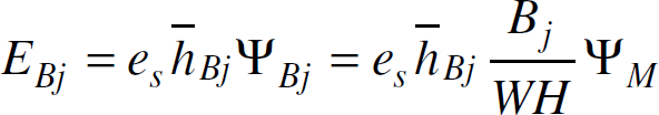
To compute (17), we need to know the values of Ψ _M and $\overline{h_{Bj}}$ . Since each data bit traverses h̅ hops to the sink on an average in the network area, according to (4), we have

$${\mathrm{\Psi }}_M=E/(\bar{h}{e}_s)$$

(18)

To compute h̅ and h̅_Bj, we need to know the average maximum one-hop progress Z̅. Since we maintain the property of uniformly distributed active sensors with density λ_min over the entire network area, the average degree g of the active sensors is a constant in all sub-regions. Hence Z̅ can be computed from (2). Given the average distance d̅ using (3), h̅ can be computed based on (4). To compute h̅_Bj, we need to know the average distance d̅_Bj from all sensors in B_j to the sink. Due to the uniformly distributed phenomenon and sensors in the sensed area, finding d̅_Bj is equivalent to finding the average distance from all points in B_j to the sink. Thus, we obtain

$$\overline{d_{Bj}}=\frac{1}{B_j}\underset{B_j}{\iint }\sqrt{(x-x_c{)}^2+(y-y_c{)}^2}dA$$

(19)

where x_c and y_c are the two coordinates of the sink. Hence, h̅_Bj is given as follows:

$${\bar{h}}_{Bj}={\bar{d}}_{Bj}/(\bar{Z}{r}_s)$$

(20)

Combining (17), (18), (19) and (20), we can obtain the value of the total energy E_Bj allocated to the sub-area B_j. Similarly, we can compute the total energy for other sub-areas. Then we need to determine how to allocate E_Bj amount of energy to each sub-region in B_j. Let A_Bj−Vk denote area of the sub-region B_j−V_k. As discussed in Section II. A, on an average, one data transmission of a node in the critical region k will forward data to a node in the (k − 1)^th critical region along a shortest hop path. One exception of this feature is V₁, since nodes in V₁ can directly send data to the sink. Therefore, the total data volume across a sub-region B_j−V₁ equals to the data generated by the entire area of B_j. The total data volume across region B_j−V_k equals to the total data generated by itself and all higher sub-regions: B_j−V_k, B_j−V_k+1,…, B_j−V_n, where V_n is the last (outmost) critical region. We define the data source areaS_Bj-Vk of a sub-region B_j−V_k as $S_{Bj-Vk}={\sum }_{i=k}^n{A}_{B_j-V_i}$ . The energy allocated to B_j−V_k is proportional to its data source area S_Bj-Vk. Let E_Bj−Vk denote the energy allocated to the sub-region B_j−V_k. Thus, we have

$$E_{Bj-Vk}=\frac{E_{Bj}{S}_{Bj-Vk}}{\sum _{i=1}^n{S}_{Bj-V_i}}$$

(21)

Since the computations of A_Bj−Vk and S_Bj−Vk are simple geometrical problems, those are omitted in this paper. For homogenous sensors, E_Bj−Vk amount of energy needs E_Bj−Vk/P _s number of sensors randomly deployed in the sub-region. The closer a sub-region is to the sink, the higher the sensor density in the sub-region. Reader may be noted that the theoretical maximum data capacity of an SSEP-NS network can be computed from (18).

C. Determination of Number of Sub-areas in the SSEP-NS Model

Another question related to the SSEP-NS model is how to determine the number of sub-areas. The number of sub-areas is affected by two parameters: one is the difficulty of sensor deployment and the other is the shape of the network area. Obviously, the difficulty of sensor deployment goes up with the increase in the number of partitioned sub-areas. When the number of sub-areas increases, area of each sub-region decreases. A very small sub-region makes random dropping of sensors difficult, and manual deployment is likely to be the only choice. For the latter, consider the SSEP-NS network shown in Fig. 14. One possible partition strategy is that we can partition the network into four sub-areas, each of which is the combination of three small sub-areas, such as combining B₁₀, B₁₁, B₁₂ into one sub-area (denoted by B′). Since the sensor density of a sub-region is proportional to its data source area, the sensor density of a sub-region B₁₀−V₁ is higher than the density of a sub-region B₁₂−V₁. On the other hand, in the combined sub-area B′, the sensors in original sub-regions B₁₀−V₁ and B₁₂−V₁ are now in the same sub-region B′−V₁. Since we uniformly distribute sensors in the same sub-region, the sensor densities for the original B₁₀−V₁ and B₁₂−V₁ are identical. However, the data volume across the original B₁₀−V₁ is larger than the one across the original B₁₂−V₁, since B₁₀−V₁ has larger data source area. This observation implies that in a network with combined sub-areas, sensors in B₁₀−V₁ will deplete their energy faster than sensors in B₁₂−V₁. For the network shown in Fig. 14, in which W = 2H and the sink is located in middle of the W edge, combined sub-areas may not lead to a serious performance degradation. In fact, we can treat the entire network area to be one single sub-area since there is no significant difference among all sub-areas. However, for a network with configuration W = H/2, the data source area of B₁₀−V₁ is more than twice of the data source area of B₁₂−V₁. Hence, the life time of sensors in B₁₀−V₁ is no more than half of the life time of sensors in B₁₂−V₁, which is not tolerable. Therefore, the number of sub-areas can not be too large or too small, and the actual selection depends on the practical network environments.

D. Discussion of the SSEP-NS Model with Insufficient Number of Sensors

Fully deploying sensors to satisfy the density requirement in a large SSEP-NS network may need a large number of sensors. Basically, we can categorize sensors into two abstract types: sensing sensors and forwarding sensors. The former only senses phenomenon and sends data to forwarding sensors and the latter only forwards the sensed data form sensing sensors. A specific sensor may perform both sensing and forwarding. But for a long term run, we can assume that there are these two abstract types of sensors existing in the system.

Due to the existence of the minimum requirement of sensor density λ_min, in an SSEP-NS network, the sensor density in an outmost critical region B_j−V_n should not be less than λ_min. Assume we deploy sensing sensors in B_j−V_n with the minimum density λ_min and the total number of sensing sensors in B_j−V_n is N_Bj−Vn(B_j−V_n does not contain forwarding sensors). To transmit the data sensed by N_Bj−Vn sensors in B_j−V_n to the sink, we need to deploy the same number (N_Bj−Vn) of forwarding sensors to each lower sub-region (from B_j−V_n−1 to B_j−V₁). Therefore, to sense phenomenon in B_j−V_n and transmit the sensed data from B_j−V_n to the sink, N_Bj−Vn sensing sensors and (k − 1) N_Bj−Vn forwarding sensors are required (k N_Bj−Vn sensors in total). Similar arguments hold for all other sub-regions, that is, for a sub-region B_j−V_k with N_Bj−Vk sensing sensors, kN_Bj−Vk forwarding sensors are needed. The minimum total sensor number N_Bj required to build sub-area B_j in an SSEP-NS network with maximum energy utilization is

$$N_{Bj}={\sum }_{k=1}^{n}k{N}_{Bj-Vk}$$

(22)

The minimum total number of sensors required to build an SSEP-NS network is

$$N_{SSEP-NS}={\sum }_{j=1}^m{N}_{Bj}$$

(23)

where m is the number of sub-areas. An SSEP-NS network with sensor number less than N_SSEP-NS leads that energy in remote sub-regions is left unused after the lifetime of the sensor network is over. Obviously, N_SSEP-NS becomes very large for a large SSEP-NS network. It may not be easy to satisfy N_SSEP-NS in practical application, if it is not impossible. A network with limited budget may use N sensors only, where N_min < N < N_SSEP-NS. In this situation, the basic SSEP-NS model needs to be modified as follows.

For an SSEP-NS network with N sensors (N_min < N < N_SSEP-NS), N_min sensors are uniformly distributed in the network area to satisfy the minimum sensor density. The remaining N′ = N − N_min sensors are used to grade the total energy in sub-regions. First, we use the similar method stated in Section IV. B to allocate N′ sensors to each sub-area. Let N_Bj denote the number of sensors allocated to the sub-area B_j. Next, we need to allocate N_Bj sensors to each sub-region B_j−V_k. Obviously sub-regions close to the sink have higher priority to deploy N_Bj additional sensors. Initially, the network area has uniformly distributed sensors with the density λ_min. The first sub-region B_j−V₁ is the bottleneck of the sub-area B_j. First, we add sensors into B_j−V₁ until it has the same data forwarding capability of B_j−V₂ to relay data from all other higher sub-regions. Since B_j−V₂ has N_Bj−V2 sensors, B_j−V₁ should also add N_Bj−V2 number of sensors to forward data from B_j−V₂. After this process, sensors in B_j−V₁ and B_j−V₂ deplete their energy at the same time and they reach the balanced condition. Now the bottleneck becomes B_j−V₁ and B_j−V₂, since B_j−V₃ has higher forwarding capability than B_j−V₁ and B_j−V₂. Then we deploy sensors in B_j−V₁ and B_j−V₂ until the first three sub-regions reach the balanced condition. Similar steps can be repeated until all N_Bj sensors are deployed.

E. SSEP-NS Routing Strategy

The routing protocol used in an SSEP-NS network is referred to as SSEP-NS protocol. In an SSEP-NS network, sensors work in one of the two modes: active mode and sleep mode. A sensor in the sleep mode turns off powers for most of its components and only runs a timer circuitry. Hence, energy consumption of sensors in the sleep mode can be ignored. When the timer expires, the sensor changes itself to the active mode. The basic idea of the SSEP-NS routing protocol is to maintain a fixed number of sensors in the active mode and other sensors in the sleep mode such that the property of uniformly distributed sensors with the minimum density λ_min holds. To balance the energy consumption, sensors change their mode after a time period.

In the SSEP-NS routing protocol, sensors need location awareness support and synchronization among all sensors. The Global Positioning System (GPS) is one choice to provide these supports. Based on the strategy discussed in the SSEP-NS model, configuration of partitioned sub-regions is determined in the network design stage and it can be represented by a set of geometrical functions. Meanwhile, the sensor density of each sub-region, the minimum density λ_min in the SSEP-NS network, and the sink location are known by sensors in this stage too.

Initially, all deployed sensors do nothing except listening to the channel. The sink at its predetermined location floods an initiation packet to all sensors containing two fields: start-time and duration Δt. The first field contains the time T_s when the network starts functioning. The duration field contains a time period Δt for which sensors are in the sleep mode if they are chosen by the selection process. Each sensor receiving the initiation packet runs the selection process to determine its next mode. If the sensor's next mode is the sleep mode, the sensor goes to sleep from time T_s to T_s + Δt. Otherwise, it will retain functioning. At the time T_s + Δt, all sensors in the sleep mode wake up. Then all sensors use the same selection process to determine their next mode for the time period from T_s + Δt to T_s + 2Δt. The same step is repeated until the lifetime of the network is over.

The selection process is used to determine whether a sensor changes itself into the sleep mode. At this time, each sensor knows its current location. From the configurations received before sensor deployment, the sensor can compute its sub-region Vj-B_k to which it belongs. Then the sensor can find the sensor density of its sub-region, denoted by λ _Bj-Vk , where λ _Bj-Vk ≥ λ_min. The sensor randomly generates a real number λ within the range [0, λ _Bj-Vk ]. If λ is greater than λ_min, the sensor's next mode is the sleep mode. Otherwise, it remains active. The selection process guarantees that the network maintains the sensor density λ_min on an average at any time. An important requirement is that the random number generators of all sensors should be independent.

To route data to the sink, many existing routing protocols can be used in an SSEP-NS network, such as the algorithm stated in [21], in which the sink floods a packet at each time T_s + nΔt (n is a non-negative integer). Each active sensor can build its forwarding path to the sink from the received packets. Hence, the sensed data can be routed to the sink along the established shortest hop paths during the time period from T_s + nΔt to T_s + (n+1)Δt. Since flooding occurs once per Δt time interval, for large Δt, the routing overhead is not significant.

F. Simulation Results

We developed a simulator to show improvements of data capacity of an SSEP-NS network compared to an SSEP network. Simulation is done in a W×H network area with W = 2H and the ratio of W and the transmission (TX) radius r_s is varied from 10 to 20. For each simulation, the network area contains only one sub-area, which is further partitioned into many sub-regions. We deploy sensors using the way we discussed in sub-section V.B based on a specific minimum density λ_min. To make a consistent view of the simulations in this paper, the minimum density λ_min is converted to an equivalent minimum average degree g_min. For all simulations, we set the initial energy for all sensors equal to 100, and e_s = 1. Each simulation terminates when more than 50% of total sensors are disconnected to the sink. All data points are computed by taking the average of 20 runs.

For each simulation run of an SSEP-NS network, the total number of sensors is known. Then we compute the data capacity and unused energy ratio for an SSEP network with the same number of sensors for comparisons. Meanwhile, since the SSEP-NS network maintains the property of uniformly distributed sensors with the minimum density λ_min at any time, we can compute (predict) the maximum potential data capacity achieved in the SSEP-NS model with the same number of sensors. Then the three set of results are compared.

Figures 15 to 18 illustrate the comparison results for the simulated performance of the SSEP-NS model, predicted performance of the SSEP-NS model and the computed performance of the SSEP model. In these figures, the curves labeled with S-NS and P-NS denote the simulated and predicted results of the SSEP_NS model, respectively. The computed results for the SSEP model are labeled with SSEP.

Figure 15

Comparison Results of Data Capacity (g_min = 8).

Figure 16

Comparison Results of μ (g_min = 8).

Figure 17

Comparison Results of Data Capacity (g_min = 12).

Figure 18

Comparison Results of μ (g_min = 12).

From these figures, we make the following observations. First, the total data capacity of a simulated SSEP-NS network (denoted by ${\bar{\mathrm{\Psi }}}_{SSEP-NS}$ ) is much larger than ${\bar{\mathrm{\Psi }}}_{SSEP}$ with the same number of sensors. The larger the network is, the larger the ratio of ${\bar{\mathrm{\Psi }}}_{SSEP-NS}/{\bar{\mathrm{\Psi }}}_{SSEP}$ . Similarly, the larger the minimum average degree g_min is, the larger the ratio of ${\bar{\mathrm{\Psi }}}_{SSEP-NS}/{\bar{\mathrm{\Psi }}}_{SSEP}$ . Second, as we predicted, the energy utilization of a simulated SSEP-NS network is much higher than the energy utilization of a SSEP network. Finally, the simulated performance of SSEP-NS networks is close to the predicted performance of the same SSEP-NS networks. Therefore, for large and dense WSNETs, the SSEP-NS model is efficient and can improve the total data capacity by one order of magnitude of the SSEP model.

VI. Concluding Remarks

In this paper, we have defined a set of static models for WSNETs. Two performance metrics, namely total network data capacity and unused energy ratio, have been defined and discussed for these static models. Due to limited energy of sensors, unlike in mobile ad hoc networks, the data capacity of WSNETs is limited too. When sink nodes are static, the maximum amount of data received by sinks is even smaller. To transmit this maximum amount of data to sinks, if the shortest hop path routing algorithm is used, there is a great amount of energy left unused after the lifetime of the network is over. For large WSNETs in the single static sink model, this energy wasting can be up to 90% of the total initial energy.

It is difficult to greatly increase the maximum data capacity and reduce the unused energy ratio by using efficient routing and MAC algorithms in these static models. However, an improvement can be made easily by using non-uniform energy distribution strategies and mobile sinks. Therefore, the SSEP-NS non-uniform sensor distribution model has been discussed and the SSEP-NS routing protocol has been proposed. In the SSEP-NS model, the network area is partitioned into sub-areas and the sub-areas are further partitioned into sub-regions. The larger the size of a sub-area is, the more sensors are deployed into the sub-area. The closer a sub-region is to the sink, the higher the sensors density in the sub-region. This sensor deployment strategy leads to non-uniformly distributed sensors in the network area. The SSEP-NS routing protocol is used to maintain the property of uniformly distributed active sensors with the minimum density at any time. This property ensures that all sensors exhaust their energy almost at the same time and leads the unused energy ratio close to 0. According to the simulation results, the SSEP-NS model can improve the total data capacity by one order of magnitude of the original SSEP model for large and dense sensors networks.

High data capacity is an important design objective in wireless sensor networks. In the static sink models, the efficiency of the MAC and routing algorithms becomes of secondary importance. To increase the data capacity, network deployment, such as distribution of node position and node energy, is a highly influencing parameter. We plan to compare the data improvement capacities of four techniques, namely variable transmit power capability of sensors [19], combination of single-hop and multi-hop routing [20], non-uniform energy distribution among sensors [18], and non-uniform sensor distribution as studied in this paper, with the same amount of total initial energy of the sensors.