
Abstract
Numerical modelling is an effective tool for predicting corrosion. We make use of a stochastic Cellular Automata (CA)-based modelling for corrosion studies at a mesoscopic scale. Physico-chemical phenomena that cannot be satisfactorily described by standard deterministic and macroscopic methods are here taken into account. In this CA modelling, materials and their environments are described by a 3D lattice, where each cell has a state. The physico-chemical phenomena are represented as simple rules that define the temporal evolution of the states of the cells. These rules can be combined to model complex systems. Our model is stochastic in the sense that the transition rules are given probabilities and diffusion in the electrolyte is modelled as a random walk. Simultaneous anodic and cathodic reactions describe the corrosion mechanisms. Special emphasis is given to the electric connection between the anodic and cathodic cells. The anodic and cathodic reactions occur simultaneously, maintaining the electric balance. In this work, we study the evolution of the generalised corrosion of a metallic surface. Two regimes are found that are determined by local acidity of the electrolyte. Uniform corrosion is predominant in the first regime, where anodic and cathodic half-reactions occur homogeneously over the surface. In the second regime, a local increase in acidity appears that induces the predominance of localised corrosion. The competition between these two regimes determines the global corrosion kinetics.
This paper is part of a supplement on the 6th International Workshop on Long-Term Prediction of Corrosion Damage in Nuclear Waste Systems.
GRAPHICAL ABSTRACT
Introduction
Alternative to empirical or semi-empirical approaches based on the extrapolation of the observations, an efficient approach for predicting corrosion consists of using models based on a mechanistic approach of corrosion phenomena [1–4]. With these methods, very low corrosion rates can be described well, even when passive layers, associated with high probabilities of localised corrosion as in the case of modern materials (stainless steel, nickel-based alloys) are present. For these highly resistant materials, localised corrosion becomes the more pernicious degradation of the material. Even though only limited portions of material are corroded, the entire metal piece can become no longer apt to service. On the modelling perspective, localised corrosion has an inherent stochastic behaviour that complicates prediction when using pure deterministic methods [5]. Therefore, when localised corrosion is an issue, the use of stochastic models is crucial. Localised corrosion is frequently combined with other types of corrosion that produce specific damages, resulting in the competition between the different mechanisms [3,6–9].
Stochastic CA enable to simulate corrosion at a mesoscopic intermediary scale while taking into account microscopic phenomena [10–15]. Moreover, the simulated durations are far longer than those attainable by microscopic approaches.
In this work, a probabilistic CA approach is used to simulate the evolution of a reactive metal surface affected by generalised corrosion. The competition of uniform and localised corrosion is studied in terms of surface morphology and corrosion kinetics. The evolution of the system is driven by the coupling between surface electrochemical reactions, diffusion and electrolyte acidity. The scenario analysed is represented schematically in Figure 1. The model is based on an approach that has been used previously to describe 2D corrosion [11,16–20]. In [21], we extended this model to 3D and applied it to study the case of an occluded corrosion cell. Here, we consider the case of a metal surface in direct contact with an aqueous environment.
Illustration of the main corrosion scenario used for CA modelling.
The paper is organised as follows: Section 2 describes the physico-chemical basis of the model, Section 3 presents the characteristics and parameters of the CA model, Section 4 presents the main results and discussions on corrosion features. Conclusions and future developments are given in Section 5.
This corrosion model lies on several assumptions: basic electrochemical reactions (anodic and cathodic) and simplified chemistry (no pollutants, only H  and OH− ions). These are common features for aqueous corrosion, regardless of the detailed nature of the metal. Localised corrosion is a multiscale phenomenon: incubation and initiation depend not only on atomic scale surface phenomena, but also on environmental conditions that can be set at a macroscopic scale. The present approach uses an intermediate mesoscopic scale that enables to highlight the general corrosion tendencies, showing the large-scale effects of a microscopically generated corrosion, simulating longer corrosion times than those that can be simulated at microscopic scale and accounting for the corrosion stochastic character generally not described at a macroscopic scale.
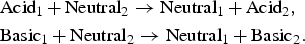
Electrochemical reactions
Electrochemical reactions summary.
Electrochemical reactions summary.
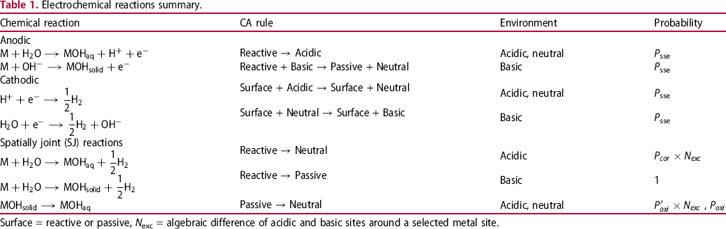
Surface = reactive or passive, N exc = algebraic difference of acidic and basic sites around a selected metal site.
Following the 2D model, we also consider the case when anodic and cathodic half-reactions occur at the same place and name them spatially joint (SJ) reactions.
Besides the electrochemical reactions, the dissolution of corrosion products  is also considered as an effect of aggressive cations. This represents the well-known destabilisation effect of aggressive ions on the passive layer.
In the case of the SSE reactions, the anodic reaction increases the acidity of its local environment by producing an H  or consuming an OH−, whereas the SSE cathodic reaction increases the basicity of the medium by consuming a proton or by water decomposition. In contrast, SJ reactions are not expected to change acidic or basic character of the solution in their vicinity. Anodic and cathodic reactions occurring at the same location, the autoprotolysis of water ensures the neutralisation of excess acidic or basic species produced by the electrochemical half-reactions.
Diffusion of H  and OH− ions is represented as a random walk. The autoprotolysis equilibrium of water will be approximated considering only the neutralisation according to

The stochastic CA model involves transformation rules and events that govern the time evolution of a fixed 3D lattice of cells. These events occur with given probabilities, as explained below.
Lattice representation
The system is represented by a discrete lattice. Each cell of the lattice is attributed a state which is determined by the dominating species in this cell. The solid cells may have three different states: M standing for bulk metal, R for reactive metal, that is metal in contact with the electrolyte and P for oxide which is supposed to give passivity to the metal. The electrolyte sites may have three states depending on the pH: A acidic, B basic and E neutral. For the CA, one can consider accessible range of concentrations between 10 and Transversal view schema of the initial lattice (a) and the corrosion evolution over the surface (b). in
in  . The upper bound is related to the concentration in a lattice site, and the lower bound is reached if one can perform averages in space or time for the presence of the sites on the lattice [21]. In this context, autoprotolysis equilibrium of water (
 ) is approximated. For pH between 4 and 10, both H
  and OH− concentrations are small for the CA description and solution is considered neutral. For pH outside this interval, we may neglect the minority species in the water autoprotolysis equilibrium. Typically, for pH less than 4, OH− is less than
  molar and vice versa for pH above 10, H
  is in this case negligible. Then only the reaction (1) between cells with acidic and basic dominating species is considered. Furthermore, we consider a metallic surface in contact with a neutral electrolyte. A 3D transversal view of the cell matrix is given in Figure 2. The neutral solution is not shown to improve visibility. The initial metallic cells at the metal/liquid interface are reactive elements, anodic and cathodic reactions occur homogeneously over the surface. In order to simulate a thickness of metal greater than the initial lattice height, the cell matrix is scrolled down as corrosion progresses.
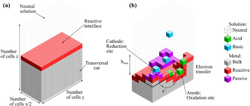
The choice of the Moore neighbourhood (with 26 neighbours) enables us to explore complex rough metal surfaces, typical of corrosion phenomena. It also ensures that the maximum available information concerning the local spatial variations of acidity–basicity is taken into account.
When reactive R or passive P sites dissolve, neighbouring M sites fall in contact with a solution site and turn into R sites. The local surrounding acidity of each site is determined by the parameter N exc which is the algebraic difference of the number of acidic and basic sites in its neighbourhood. Thus N exc is positive for acidic pH and negative for basic pH.
Electrochemical reactions are translated into CA transition rules. The second column of Table 1 shows a summary of the transition rules of the model and their probabilities. Anodic and cathodic half-reactions occur simultaneously at separate sites. Because these half-reactions are integrated in a closed electric circuit (to preserve the global electro-neutrality of the system), the corresponding sites must be electrically connected through the solid and the electrolyte. In the solid part, this means that the sites must be joined by a path of R, M or P (because in this work, we supposed that oxides are electronic conductors) sites, whereas an ionic transfer occurs in the electrolyte part by diffusion.
Let us point out that the irregular dissolution of the metal produces a rough surface which favours the creation of islands. These islands have been shown to be small in the case of the occluded cell [21]. Here, we study the role of the islands in the dynamics and evolution of the system in a different configuration. Instead of removing the islands upon detachment, we assume they progressively dissolve with probability P diss.
Diffusion
Acidic and basic cells diffuse through the electrolyte, according to transition rules that model the Brownian motion of the ionic species, as in [21]. For a cell 1 in contact with a cell 2, diffusion corresponds to swapping the content of the cells, i.e. their states and can be written as follows
If a collision occurs between an acidic and basic cell, they annihilate turning into neutral solution cells:

The diffusion characteristic length l over a time t is determined using the mean square displacement equation  , where d is the dimensionality considered (here
  ) and D is the diffusion coefficient of the ions. For Moore neighbourhood (26 neighbours), discretisation length a, the characteristic diffusion time is
 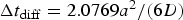 [21].
[21].
H  and OH− ions are assumed to diffuse with a common mean diffusion coefficient
  found in the literature [22]. In the simulation, to accelerate calculations, we compute Equation (2) also for the symmetric case with inverted content of cells 1 and 2. This corresponds, for the simulation algorithm, to dividing the simulation diffusion coefficient by a factor 2 and the corresponding time step is multiplied by 2. Assuming
  , we obtain for the simulation time step
 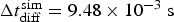 .
.
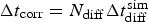
The algorithm has been organised as in [21]. Note that in each main loop corresponding to a corrosion step, there is an inner diffusion loop which is performed N diff times. N diff then stands for the rate between corrosion ( ) and diffusion (
 ) characteristic time steps according to
  . Where
  , which means that for the corrosion rates and values of a chosen, the elementary diffusion step (two sites swapping process) is faster than corrosion reactions. Diffusion algorithm is a parallelised swapping procedure of species OH− and H
  . Faster diffusion algorithms have been proposed in the literature [23], but they are not well adapted for the non-local anodic and cathodic autocatalytic surface reactions. Moreover, a precise balance between OH− and H
  species must be maintained.
The lattice is composed of  cells. This value has been chosen in order to obtain sufficiently accurate statistical results. Periodic boundary conditions have been applied at the edges of the system in the horizontal directions. To focus on the effect of SSE reactions, we keep only the passivation effect in SJ reactions (i.e. setting
 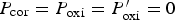 in SJ probabilities, see Table 1). This passivation effect in basic environment is similar to that of Iron (see Pourbaix diagram for Iron [24]). In the simulation, the frequency of a corrosion trial step is set by the parameter for SSE reactions with a probability of
  . Note that the effective occurrence of the corrosion step depends on other events like presence of acidic of basic species in the vicinity.
Results and discussion
When simulation starts, anodic and cathodic reactions are evenly distributed over the reactive surface. An anodic reaction can occur in acidic or basic environment (see Table 1). The number of anodic and cathodic reactions is linked to the number of electrons exchanged and given through P sse probability. In neutral or acidic environment, it leads to the dissolution of a reactive cell and the creation of an acidic cell, which means that there is an autocatalytic effect. In a basic environment, it produces passivation of the metal that contributes to the local protection of the material.
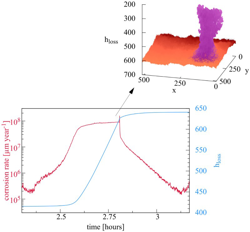
Dynamics and corrosion kinetics of the system are determined by the competition between annihilation of ionic species in the electrolyte, passivation and autocatalytic metal dissolution in acidic environment as illustrated in Figure 3. The first regime corresponds to uniform corrosion, during which the annihilation mechanism is sufficient to keep a homogeneous pH, see Figure 3(a). However, this homogeneity is not perfect. In Figure 3(a), we can observe that corrosion is not uniform, small patches of oxide are visible. This indicates that this is a stochastic process. The evolution then shows that some patch may lead to an instability. Two opposite effects are present. On the one hand, neutralisation has the tendency to restore neutral uniform solution and therefore uniform surface. However, the separate SSE half-reactions tend to destabilise the systems. They tend to create separate acidic and basic regions and their process is somewhat autocatalytic. The cathodic basic regions sustain passivation; therefore, no anodic reaction can take place, catalysing further cathodic reaction. But on an anodic site, acidity opposes passivation and anodic reaction can further take place. This effect leads to small acidic or basic volumes in the vicinity of the surface. If most inhomogeneities are small and due to neutralisation disappear, one should also note that mechanism of neutralisation proceeds mainly on the interface between acidic and basic regions leading to a much less efficient neutralisation process than the the equivalent volume reaction and therefore slower kinetics. It is then possible that diffusion is not sufficient to annihilate these local excesses and due to the autocatalytic mechanism this is the onset of the spatial separation of different regions which may now stabilise and further grow. Note that the local excesses of one or the other acidic or basic species as a result of the anodic and cathodic half-reactions have concentration values far larger than that of the neutral water autoprotolysis equilibrium. The other species of the autoprotolysis equilibrium can then be considered negligible, this is why it has been neglected in our CA representation. This transition is illustrated in Figure 3(b). The separation of zones induces a predominance of localised corrosion and increasing corrosion rate. The metal in basic zones passivates, reducing the local corrosion rate (see Table 1). The metal in the acidic zone increases the local corrosion rate due to the autocatalytic effect. As a result of this heterogenous corrosion growth, a passivated peninsula appears (see Figure 3(c)). This emergence of metal peninsulas has been experimentally associated with cathodic protection [25]. One also observes that the essentially anodic metal surface around the peninsula is now practically free of passive sites, illustrating the above-mentioned autocatalytic scenario.
Generalised corrosion evolution for  ,
,  and
and  . On the left, only metallic surface is shown, whereas on the right acidic and basic species is also shown. (a) Anodic and cathodic half-reactions are evenly distributed over the surface, uniform corrosion (b) autocatalytic effect of anodic reactions induces a separation of acidic and basic zones, localised corrosion is predominant (c) passivated metal in the basic zone forms a metal peninsula (d) passive metal is detached from the main corrosion front, corrosion kinetics decreases.
As corrosion progresses, the size of the metal peninsula increases. The peninsula is associated with heterogeneous corrosion corresponding to cathodic sites on the passivated peninsula and anodic sites on the metallic surface around the peninsula. This leads to acidic zones situated closer to the surface around the peninsula and a basic zone surrounding the peninsula and thus extending further into the solution. As the peninsula grows, the anodic, acidic region may close in onto the base of the peninsula causing the rupture of the metallic connection and leading to its detachment and formation of an island. The appearance of such metallic islands can be related with the chunk effect 1 [18,26–30]. This island is progressively dissolved with probability P diss. Its advancing dissolution results in the emergence of a large number of small islands. Once the island detaches, the metallic surface around the detached island sees new passive sites appearing and the main corrosion front reverses to a configuration similar to the initial stage with scattered patches of passive sites. This resolves to anodic and cathodic half-reactions occurring evenly over the entire surface. As a consequence, uniform corrosion becomes predominant and the spatial distribution of local pH is again homogeneous. This is illustrated in Figure 3(d).
We can then conclude that the corrosion process, starting with generalised corrosion switching to localised corrosion with formation of randomly distributed metal peninsulas and leading to the production of islands, follows a cycle. The occurrence of the new peninsulas is localised at random on the corroded surface. This is one of the main features of the morphological evolution of the system. Figure 4 shows the cumulated number of corroded cells N corr (i.e. the number of initially metallic cells M that have been transformed into electrolytes A, B or E cells) and the number of SSE reactions for each time step. The latter is related to corrosion kinetics. Low corrosion rate is evident in the first regime (region 1), corrosion increases after the separation of acidic and basic zones (region 2), metal is detached and corrosion rate decreases (region 3), corrosion rate decreases to its initial value because of the predominance of uniform corrosion (region 4). The effect of the corrosion rate is visible on the evolution of the number of corroded sites.

Number of corroded cells and SSE reactions versus number of time step. ,  .
.
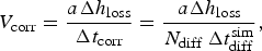
The average corrosion depth is defined as (a) Corrosion depth as a function of time for different values of N diff. Dashed lines represent the size of the largest detached island,  where N corr is the number of corroded cells which is proportional to a volume and
  the surface dimension in number of cells. Cells are corroded by SSE anodic half-reaction or by dissolution in the case of islands. Figure 5(a) shows the evolution of h loss for different values of N diff. The scrolling of the matrix accompanying corrosion progress is made by adding metal cells at the bottom and erasing top matrix solution cells keeping balance between acidic and basic sites. Time separating successive localised corrosion events increases with N diff.
 . (b) Same quantity but different values of P diss,
  .
.
Figure 5(b) shows the evolution of h loss and the maximum size of islands for different values of the P diss. The starting time for the localised corrosion regime has a stochastic behaviour independent of P diss. At the end of the localised corrosion regime, large island detachment occurs. We note that increasing dissolution rate, we observe higher frequency of detachment events, as well as larger sizes of detached islands.
Figure 6 shows the number and average size of islands. In the uniform corrosion regime, their number is relatively small for instance for (a) Number and (b) average size of islands for different values of P diss.  , only a few hundreds with small size only a few sites. Note that the number of islands is larger for smaller values of P diss, but this is due to the slower dissolution of islands leading to their accumulation in time. Their size remains small. During the localised corrosion phase, the number and size of islands increases abruptly. In this regime, this is due to the dissolution of the large peninsula into a large number of small islands. Then, the average size drops sharply when the peninsula is totally dissolved and the system resumes uniform corrosion.
 .
.
It is possible to define a corrosion rate V corr from the derivate of the corroded depth h loss using the following equation
(a) Evolution of the corrosion rate for different values of N diff. Characteristic values for fast and low corrosion regimes, dashed lines. (b) Average corrosion rate as function of N diff for the characteristic values of fast (blue) and low (red) corrosion regimes. Linear regressions in dashed lines. Square points are extrapolated values of N diff for more realistic corrosion rates.
 is the time step of the corrosion. The time evolution of the corrosion rate is represented in Figure 7(a) for different values of N diff. Two main characteristic values appear: a peak value that corresponds to the localised corrosion regime (between 3 and
  ) and a low value that characterises the uniform corrosion regime, which is between 1 and
  . In general, the corrosion rate will be lower as the neutralisation mechanism is more efficient, that is large N diff and successive localised corrosion phases will be more spaced in time.
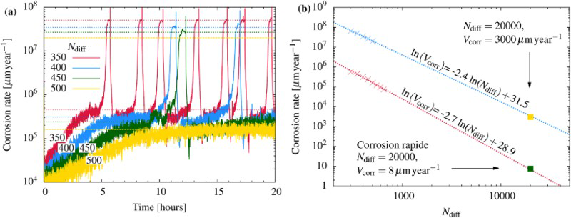
The simulated corrosion rate values (between  and
and  ) are far greater than those observed experimentally for long-term predictions [31], which are close to
  . The corresponding value of N diff is much larger than what we can simulate. Figure 7(b) shows the average corrosion rate as a function of N diff for the fast and low corrosion regimes. Extrapolating the values of the low corrosion rate to match experimental typical values of generalised corrosion, we find that N diff should be 20 000. The localised corrosion event will be rarer. However, such events may occur in longer time scales such as those purposed for operational devices. Extrapolating (yellow square) the high corrosion rate values, we can deduce a value of
  for localised corrosion rate. Such a value is clearly much larger than uniform corrosion expected in nuclear geological storage. Note that this value may be altered if we take into account that the diffusion of ions occurs in the presence of corrosion products and in addition, large N diff requires large simulations lattices, which are difficult to implement presently.
We use a probabilistic CA model to study the competition between localised and uniform corrosion. It is applied to the case of generalised corrosion over a reactive surface. This model couples spatially separated anodic and cathodic half-reactions with solution local properties (in particular acido-basic effects). Two regimes are found depending on local acidity of the electrolyte. A first regime, characterised by the predominance of uniform corrosion where anodic and cathodic half-reactions are distributed homogeneously over the surface. A second regime characterised by a predominance of localised corrosion, where in the anodic regions, an autocatalytic effect increases the local corrosion rate. On the contrary, the cathodic reaction promotes passivity and locally protects the surface.
The morphological evolution of the surface exhibits metal islands’ detachment during the localised corrosion regime. This phenomenon has been directly related to the chunk effect and has been described only by CA.
Regarding quantitative results, this work presents corrosion predictions of a scenario where corrosion rate abruptly increases due to a localised corrosion attack. It is important to highlight that the simulated durations are in the range of hours. Even if some investigation is still needed to obtain representative corrosion rate values, this is an important progress in the development of mesoscopic models, taking into account that our simulations are based on electrochemical reactions that occur at a microscopic scale.
Future development for this model are aimed at including other phenomena that influence corrosion such as, among others, IR drop, precipitation of species at the surface and cations influence and improving the diffusion algorithm in order to simulate the extrapolated corrosion rate values.