Sage Journals: Discover world-class research

Abstract

Linear friction welding (LFW) is a solid-state joining process that significantly reduces manufacturing costs when fabricating Ti–6Al–4V aircraft components. This article describes the development of a novel 3D LFW process model for joining Ti–6Al–4V. Displacement histories were taken from experiments and used as modelling inputs; herein is the novelty of the approach, which resulted in decreased computational time and memory storage requirements. In general, the models captured the experimental weld phenomena and showed that the thermo-mechanically affected zone and interface temperature are reduced when the workpieces are oscillated along the shorter of the two interface contact dimensions. Moreover, the models showed that unbonded regions occur at the corners of the weld interface, which are eliminated by increasing the burn-off.

Keywords

Linear friction welding process modelling titanium alloy material flow geometry DEFORM

Introduction

Linear friction welding (LFW) is a solid-state joining technology that is commercially established for fabricating titanium alloy integrated bladed disks (Blisks) for the aerospace industry [1, 2]. Figure 1(a) shows an example of a blisk fabricated by the LFW process. Owing to the many benefits the process offers, it is finding increasing interest for the manufacture of Ti–6Al–4V aircraft structural components. Components machined from a solid block are expensive owing to the proportionally large amount of material that is purchased compared to the amount that remains after machining [3]. LFW reduces the material required to make a component by joining smaller workpieces to produce a preform, which is subsequently machined to the desired dimensions [1, 4], as shown in Figure 1(b). This brings substantial improvements to buy-to-fly ratios, which significantly reduces manufacturing costs [1, 2, 5]. The linear friction welded components also have a comparable strength and quality to machined parts [6]. Despite the increased interest, the process has experienced limited industrial implementation outside of blisk manufacture [7, 8]. This is partly due to limited process understanding.

Figure 1

(a) A blisk fabricated by LFW and (b) a fabrication of a Ti–6Al–4V preform using the LFW process. The as-welded structure can be seen on the left side of the figure and the final machined component on the right. Images courtesy of TWI.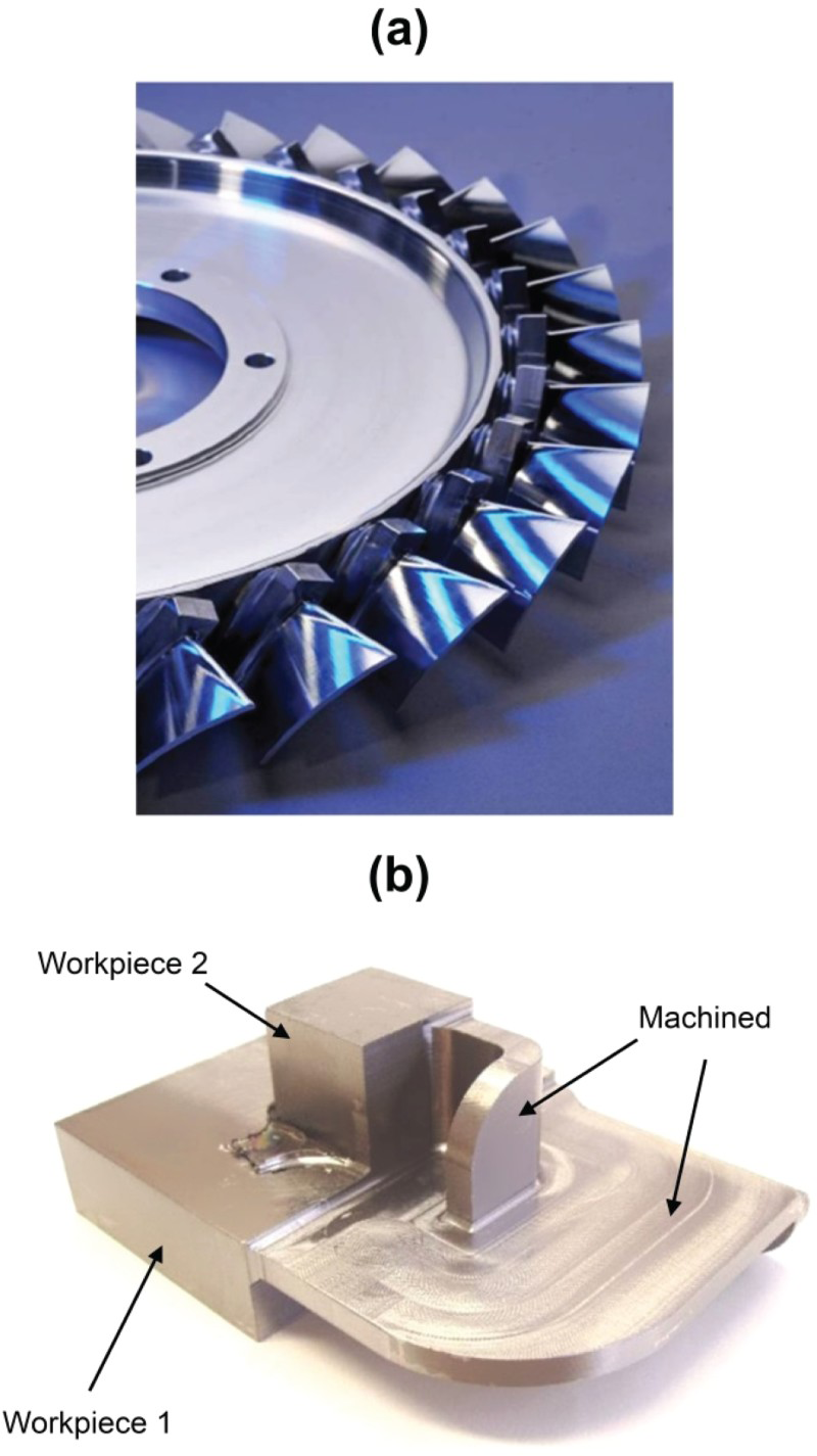

LFW works by oscillating one workpiece relative to another while under a compressive force [9 -12]. Although a continuous process, Vairis and Frost [10] noticed that LFW occurs over four unique phases:

Phase 1 – initial: Microscopic contact exists between asperities on the two surfaces to be joined and heat is generated owing to friction. The asperities soften and deform, increasing the true area of contact between the workpieces. Negligible axial shortening (burn-off) in the direction of the applied force is observed during this phase.

Phase 2 – transition: The heat due to friction causes the interface material to plasticise and become highly viscous. This causes the true area of contact between the workpieces to increase to 100% of the cross-sectional area. Heat conducts away from the interface, softening more material, and the burn-off begins to occur owing to the expulsion of the viscous material from the weld interface.

Phase 3 – equilibrium: A quasi-steady-state condition is achieved and the axial shortening (burn-off) occurs at a nearly constant rate through the rapid expulsion of interface material, forming the flash.

Phase 4 – deceleration and forging: The relative motion is ceased and the workpieces are aligned. In some applications, an additional increased forging force may be applied to help consolidate the weld.

Owing to the rapid nature of LFW, it is often difficult to understand the process using experiments alone. Numerical modelling offers a pragmatic method for understanding the flash formation, interface contaminant removal and the thermal histories, helping researchers to better understand the process [1, 5, 13, 14]. Much of the numerical modelling work on Ti–6Al–4V consists of 2D models, which have been shown to successfully provide an adequate insight into many of the phenomena associated with LFW. The main advantage of 2D models is the quicker simulation times, owing to the reduced element count and terms included in the heat and mass flow equations. This makes 2D models particularly suitable for parametric studies. However, by their nature, these models are unable to replicate the flash in the direction perpendicular to the direction of oscillation, therefore limiting full process behaviour understanding [5]. There is a need to use 3D models to provide a qualitative insight into the full multi-directional flow behaviour, particularly to understand the flow at the corners of the workpieces – something 2D models cannot do. Consequently, during the last few years, considerable effort has been made to develop 3D LFW process models to give better process insight. For example, Fratini et al. [15] used 3D models of steel workpieces to investigate the effects of the process input parameters on the weld temperature. The work showed that the temperature increases with the frequency and pressure. In contrast, Li et al. [16] modelled steel workpieces and found the interface temperature during phase 3 to be relatively insensitive to the processing conditions. Grujicic et al. [17 -19] developed a 3D LFW process model to investigate the microstructural evolution in Ti–6Al–4V welds and precipitation-hardened martensitic stainless steel welds. The results were found to be in good agreement with experimental counterparts. Sorina-Müller et al. [20] developed a 3D model to compare the weld temperatures of a ‘prismatic’ and a ‘blade-like’ geometry for Ti–6Al–2Sn–4Cr–6Mo; the larger prismatic geometry had a higher interface temperature. Li et al. [21] analysed high-speed photography of the LFW process and noted that the workpieces do not oscillate in a rigid manner. In fact, it was noticed that the workpieces can move in the tooling, which generates a ‘micro swing’ effect. A 3D LFW process model was produced to investigate this effect for Ti–6Al–4V welds. The models showed that the burn-off rate increased with larger angles of micro-swing, which was due to one workpiece digging further into the other and extruding more material per cycle. According to Li et al. [21], the different micro-swinging angles had negligible effect on the interface temperature at the centre of the weld. Bikmeyev et al. [22] used a 3D model to investigate the mechanisms behind the formation of the plasticised layer (start of phase 2). The model demonstrated that the plasticised layer initially forms at the centre of the weld, which was confirmed with experiments. Nikiforov et al. [23] and Bühr et al. [24] used a 3D approach to investigate residual stress formation in Ti–6Al–4V linear friction welds. The results showed that residual stresses can be minimised by appropriate selection of the process inputs, with higher applied pressures and lower rubbing velocities reducing the peak tensile stress values.

The present article reports on the development of a novel 3D LFW process model for joining Ti–6Al–4V. The purpose of the article is twofold. The first is to provide insight into the effects of the workpiece geometry on the multi-directional material flow behaviour of Ti–6Al–4V welds. The second is to inform the reader of the novel modelling approach benefits, hopefully providing a platform on which further 3D modelling investigations may be based.

Methodology

Experimental

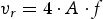
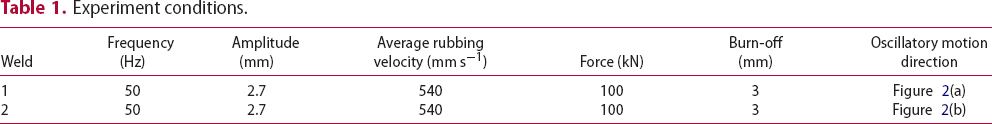
Several experiments were completed to provide input and comparison data for the models discussed in the subsequent sections. The workpiece geometry and experimental conditions used are displayed in Figure 2 and Table 1, respectively. For Table 1, the average rubbing velocity, , was defined as (1) The Ti–6Al–4V workpieces used for the experiments had a bimodal alpha–beta microstructure. All of the experiments were completed using the FW34 LFW machine at TWI, Cambridge, UK. Before welding, the workpieces were cleaned with acetone.

Figure 2

Workpiece dimensions where the oscillatory motion took place in the: (a) ‘x’ direction and (b) ‘y’ direction. Note that 60 mm represents the height of a single workpiece.

Table 1

Experiment conditions.

Weld	Frequency (Hz)	Amplitude (mm)	Average rubbing velocity (mm s⁻¹)	Force (kN)	Burn-off (mm)	Oscillatory motion direction
1	50	2.7	540	100	3	Figure 2(a)
2	50	2.7	540	100	3	Figure 2(b)

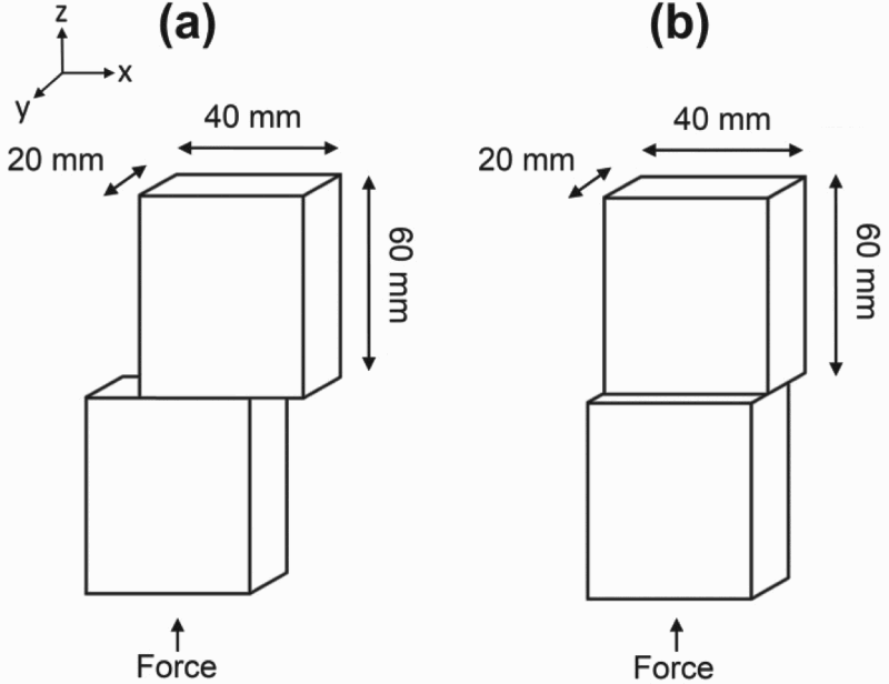
The amplitude and burn-off displacement histories were recorded from the experiments. These values from phase 2 onwards were used as input data for the models, as will be discussed in section ‘Plastic flow model’.

Metallographic samples were produced from the experimental welds. The sectioned samples were mounted and then ground using 240, 1200, 2500 and 4000 grit silicon carbide papers. After grinding, the sectioned samples were polished using colloidal silica on a micro-cloth and etched using a 3% hydrofluoric acid solution. The metallographic samples were viewed under a refractive microscope to determine the extent of the thermo-mechanically affected zone (TMAZ) so that comparisons with the models could be made.

Development of a 3D model

McAndrew et al. [1, 4, 5] previously reviewed the different LFW finite element analysis (FEA) approaches that are documented in the literature. An increasingly popular approach for the modelling of titanium alloys – specifically Ti–6Al–4V – is the ‘single-body approach’ [1, 5, 13, 25, 26]. This approach is based on the following theory: Before phase 2 takes place, there is negligible macroscopic plastic deformation. Once phase 2 begins, the process may be modelled as a single body owing to there being approximately 100% true interface contact. A temperature profile needs to be mapped onto the single body model to account for the heat generated during phase 1. The high temperature at the region corresponding to the weld interface allows the material at the centre of the model to deform in preference to the cooler surrounding material, allowing the single body to represent two individual workpieces. Owing to the adhesion of the interface material being modelled, much better replications of the flash morphology are produced. The ‘single-body approach’ forms the basis for the 3D model in this work. Consequently, the modelling work is discussed in two sections. First, a purely thermal model to account for the heating of the workpieces during phase 1, and second, a plastic flow model to account for the material flow during the oscillatory motion, i.e. phases 2, 3 and 4. The FEA software package DEFORM V.11 was used for the modelling work.

Thermal model

The thermal model presented in this paper is based on the same approach used in previous work [1, 5, 14]. This initially involved modelling the workpieces with a 2D model, the geometry of which is displayed in Figure 3(a). The workpiece contact with the tooling extended to within 5 mm of the weld interface as occurred in the experiments. A uniform mesh size of 0.5 mm was used across the model. Temperature-dependent thermal conductivity, specific heat and emissivity data from the DEFORM software's library were used [27]. The convective heat transfer coefficient was assumed [13] to be 10 W/(m² K); and the conductive heat transfer coefficient with the tooling was assumed [13] to be of 10 000 W/(m² K). The temperature of the environment was assumed to be 20°C.

Figure 3

Developed 2D thermal model showing: (a) the heat flux approach and (b) a 3D illustration of the thermal profile generated at the end of phase 1.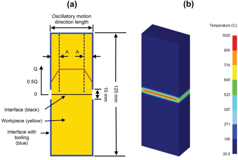

A uniform heat flux (Q) was applied across most of the workpiece interface which was linearly reduced to 50% of this value from an amplitude (A) away from the edge as shown in Figure 3(a). The reduction at the edges was due to the sinusoidal movement of the workpieces – the point at the corner was only in contact with the other workpiece 50% of the time. The heat flux was determined by dividing the average power input for phase 1 – see equation (2) – by the average in-contact interface area of the workpieces determined in previous publications [1, 14]. 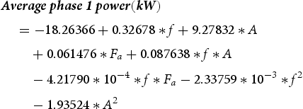(2) where A is the amplitude (mm), f is the frequency (Hz) and F_a is the applied force (kN).

The interface temperature at the end of phase 1, irrespective of the process inputs, has been shown to reach approximately 1000°C for Ti–6Al–4V linear friction welds [14]; consequently, the heat flux was applied until the elements at the interface had achieved this temperature. Once complete, the results from the 2D models were extruded into the third dimension to give full geometric representation of the conditions in Figure 2. This was deemed an acceptable approach as previous 3D LFW process models have shown that there is minimal difference in the temperature profile transverse to the direction of oscillation during the early stages of the process [18]. Figure 3(b) illustrates an example of the generated thermal profile at the end of phase 1.

Plastic flow model

3D single-body plastic flow models were set up in accordance with the dimensions shown in Figure 4(a,b) so that the conditions in Table 1 could be modelled. As can be seen, several approaches were employed to reduce the amount of elements required and therefore the computational time. First, the 3D models were specifically designed to focus on the weld region, i.e. 10 mm either side of the weld interface for the geometry displayed in Figure 2. Second, only half of the volume of the workpieces was modelled, which was deemed acceptable because the process is approximately symmetric about the x–z plane along the centre of the workpiece, therefore giving full weld representation [28].

Figure 4

Plastic flow models showing the dimensions and symmetry plane for the conditions oscillated in the: (a) 20 mm interface dimension, and (b) 40 mm interface dimension. Note that the grey objects represent the displacement dies and are not included in the dimensions.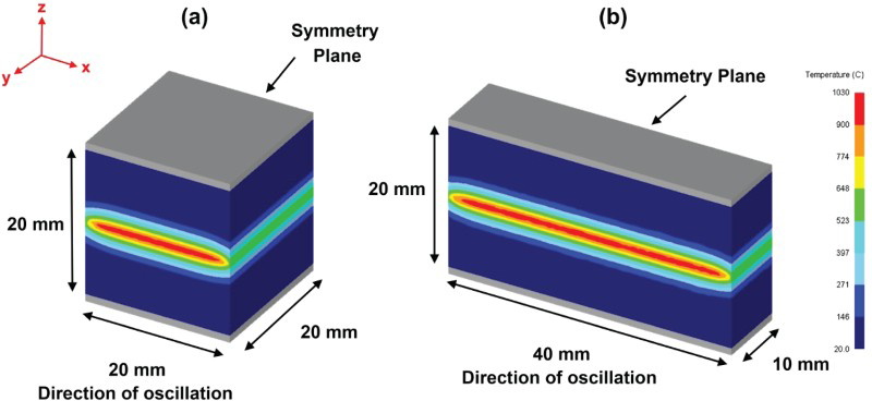

For 2D LFW process models, a mesh with an element size below 0.25 mm [1, 5, 13, 25] is sufficient to capture the plastic deformation at the weld interface. 3D LFW process models require substantially more time than 2D models to complete a simulation owing to the increased element count, and terms included in the heat and mass flow equations. As such, many authors, when using DEFORM-3D to model friction welding-based processes, often use slightly larger elements at the plastic deformation zones. For example, when modelling the friction stir [29, 30] and friction stir spot [31] welding processes, the plastic deformation zone was meshed with elements of between 0.8 and 0.5 mm in size. Therefore, a uniform mesh was applied throughout the workpieces which had elements that were approximately 0.5 mm in size. The generated thermal profiles from section ‘Thermal model’ were then mapped onto the plastic flow models, as shown in Figure 4(a,b).

The constitutive material data used was the same as previously reported [5, 13]. In summary, the material flow stresses were obtained from stress and strain curves for temperatures, strains and strain rates up to 1500°C, 4 and 1000 s⁻¹, respectively. The values for the thermal conductivity, specific heat capacity, emissivity, and heat transfer to the tooling and environment were identical to the values used for the thermal models.

Unlike previous work documented in the literature [1, 5, 13, 25], the modelling approach presented in this paper used a ‘retrospective’ analysis. This meant that the amplitude and burn-off displacement histories were taken from the experiments and used as process inputs for the models; herein lies the novelty of the LFW modelling approach. The advantage of this approach is that the process inputs can be defined as ‘paths’ instead of ‘forces’, allowing the conjugate gradient solver to be used, which, according to the DEFORM users’ manual, reduces the computational time and storage memory. The oscillation and burn-off displacements were prescribed on the lower and upper dies, respectively. Each model was given a time-step so that it approximately travelled a third of the interface mesh element thickness per iteration. The thermal and mechanical aspects of the analysis were coupled. A re-mesh was initiated every 0.1 s for all cases. Several responses were recorded from the models, including the thermal fields, strain rates and extent of flowing material.

Results and discussion

Experimental displacement histories

The experimental displacement histories from phase 2 onward that were used for input data for the LFW process models are displayed in Figure 5. Note that the axial shortening exceeds the specified burn-off values displayed in Table 1. This was due to extra material being expelled from the interface during the ramp-down of the oscillatory motion, which occurs once the desired burn-off has been achieved. Another observation worth commenting on is the burn-off rate. For the conditions in Figure 5(a), the steady-state burn-off rate was 6 mm s⁻¹, while in Figure 5(b) it was 7.1 mm s⁻¹. This observation was reported previously [1] and is a consequence of the material being expelled more quickly when the workpiece is oscillated along the shorter of the two interface contact dimensions.

Figure 5

Experimental displacement histories from phase 2 onward for a frequency, amplitude, applied force and burn-off of 50 Hz, 2.7 mm, 100 kN and 3 mm, respectively for the experiment oscillated in the: (a) 40 mm interface dimension and (b) 20 mm interface dimension.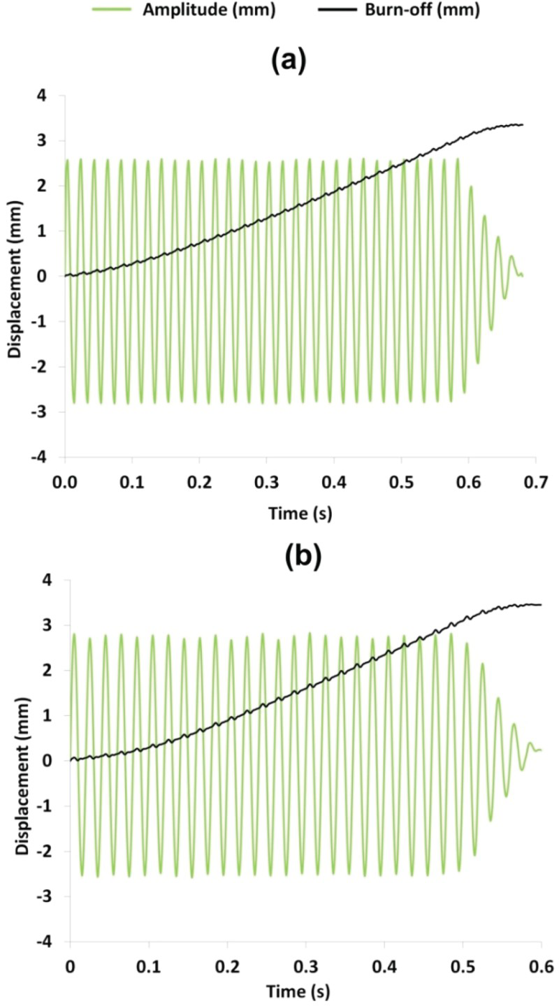

Material flow and thermal fields

TMAZ and flash observations

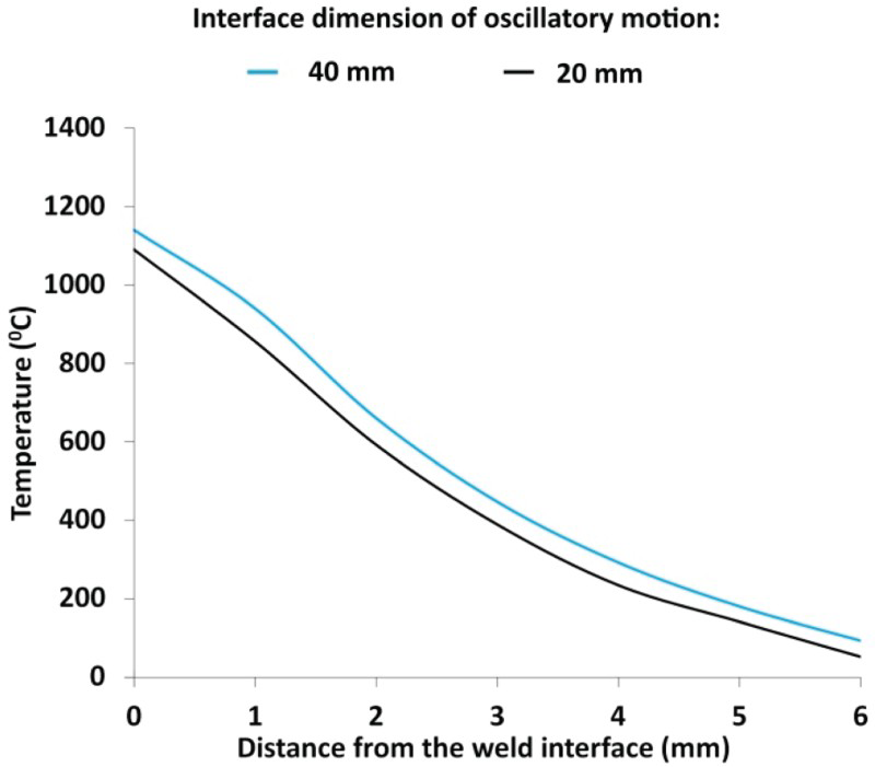
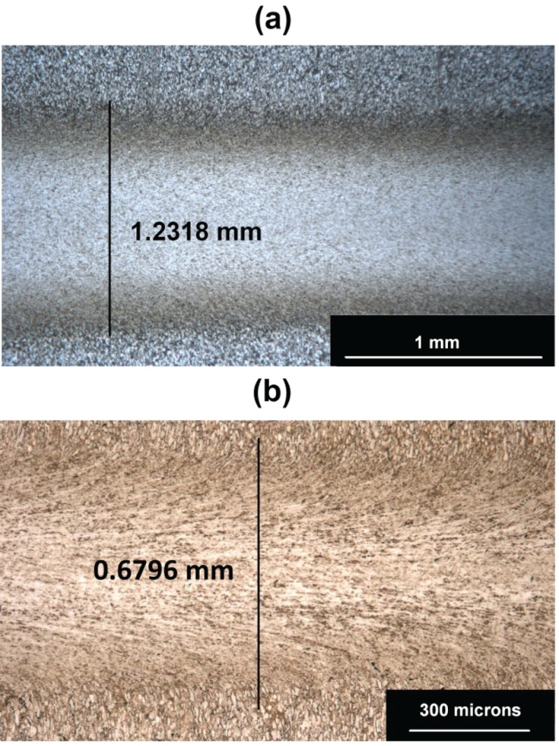
As shown in Figure 6, and in agreement with previous 2D FEA work [1, 5], the 3D models showed that the boundary temperature between the rapidly flowing flash and material with negligible flow approximately corresponded to the β-transus for this alloy (980°C to 1010°C). This is because significant material softening occurs at this temperature. For an identical combination of process inputs, the models showed that the extent of the TMAZ decreased when the workpieces were oscillated along the shorter of the two interface contact dimensions, i.e. the 20 mm dimension. This was because this condition had a higher burn-off rate, which increased the rate at which hot material was expelled from the weld interface [1, 32]. This reduced the time the heat had to conduct back from the weld interface, reducing the extent of the material above the β-transus and therefore the TMAZ, as can be seen in Figure 7. According to the models, the TMAZ was 1.45 mm for the weld oscillated along the 40 mm interface dimension and 0.76 mm for the weld oscillated along the 20 mm interface dimension. The experimental welds that the models replicated support this observation, as shown in Figure 8. The experimental values were slightly lower than the models, which was probably due to the assumptions associated with the models, such as choice of mesh size, flow stress and thermal conductivity data. Figure 8 also shows that the weld interface had a fine, recrystallised microstructure, surrounded by deformed parent material grains, which is in agreement with the literature [1, 5, 33, 34]. Moreover, the weld oscillated along 20 mm interface dimension had a decreased interface temperature, as shown in Figure 7. This was because the material farther back from the interface was much cooler in this weld. When this cooler material reached the weld interface, it effectively cooled the weld, producing a lower interface temperature, which is in agreement with the literature [1, 32]. Based on the above findings, there may be a benefit to oscillating the workpieces along the shorter of the two interface–contact dimensions when producing Ti–6Al–4V welds as the lower temperatures may reduce the generated residual stresses [23, 24, 26, 33].

Figure 6

Appearance of the models for: (a) the experiment oscillated in the 40 mm interface dimension and (b) the experiment oscillated in the 20 mm interface dimension.

Figure 7

Thermal histories recorded from the models during phase 3 (equilibrium phase) of the LFW process.

Figure 8

Experimental TMAZ for: (a) the experiment oscillated in the 40 mm interface dimension and (b) the experiment oscillated in the 20 mm interface dimension.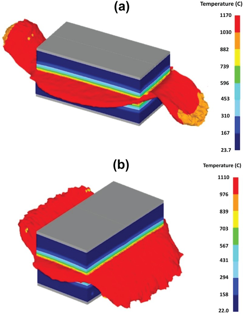

Despite the models capturing the weld phenomena of the experimental TMAZ, some criticisms of the models must be made. As shown in Figure 6, the interface mesh appears to have been too large to capture the distinct ‘rippling’ effect that was observed in the flash of the experimental welds. Furthermore, the peak strain rates recorded from the 3D models were between 440 and 500 s⁻¹ – far lower than the values of between 800 and 1500 s⁻¹, predicted by comparable 2D process models with a finer mesh [1, 4, 5]. Modelled strain rates are known to be under-predicted when the mesh element size is increased in LFW process models [13]. An obvious solution would be to decrease the element size of the 3D models; however, this would increase the computational time. The 3D models in this work already took between 4 and 6 weeks to complete a simulation on a high performance PC, even with the ‘retrospective’ analysis being employed; far longer than the 12 h required for a comparable 2D LFW process model [4].

Interface corner phenomena

Addison [34, 35] noted that the corners of the weld interface can contain a small, unbonded region, as shown in Figure 9(a). Insufficient bonding at the interface results in welds having poorer mechanical properties [34, 36]. As such, the developed 3D models were used to investigate the material flow at the corners of the weld interface, something that has not been investigated before. As shown in Figure 9(b), the unbonded regions at the corners are very noticeable at low burn-off values. According to the models, as the burn-off progresses, heat from the flash and interface conducts into the corners causing them to soften and plastically deform. This results in the corner material merging with the rest of the interface, forming a bond, as shown in Figure 6, eliminating a source of inferior mechanical properties [34, 36].

Figure 9

Weld interface corner bonding: (a) an unbonded region in an experimental Ti–6Al–4V ‘T’ joint linear friction weld (image courtesy of TWI) and (b) FEA showing an unbonded region at the interface corners for a low burn-off.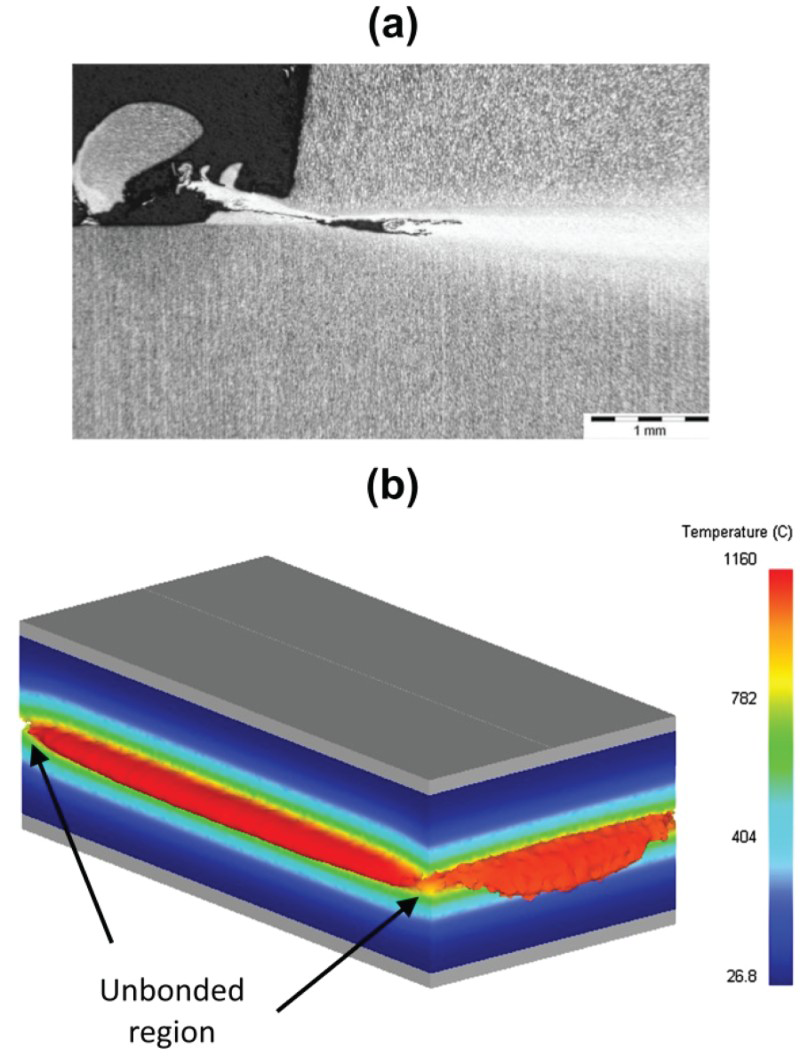

Conclusions

The primary conclusions from this work are as follows:

A novel LFW process modelling technique, the ‘retrospective’ analysis, was presented. The advantage of this technique is that the process inputs can be defined as ‘paths’ instead of ‘forces’ allowing the conjugate gradient solver to be used, which decreases the required computational time and memory storage. The limitation of this approach is that prior knowledge of the displacement histories must be known.

An interface mesh element size of 0.5 mm appeared to be sufficient to capture the general experimental trends of the process, such as the thermal fields and the extent of the TMAZ. However, these elements were too large to capture the finer material flow phenomena, such as the distinct ‘rippling’ effect in the flash.

The models showed that the TMAZ and weld interface temperature are reduced when the workpieces are oscillated along the shorter of the two interface contact dimensions.

Unbonded regions can occur at the corners of the weld interface. According to the 3D LFW process models, these unbonded regions can be eliminated by increasing the burn-off.

The work showed that although the 3D models captured the multi-directional flow behaviour of the process, the computational time requirements were still large, even with the retrospective analysis being employed. This suggests that parametric studies are better achieved by 2D LFW process models.

Footnotes

Disclosure statement

No potential conflict of interest was reported by the authors.

Data access

All data supporting this study are openly available from the Cranfield University repository at https://dx.doi.org/10.17862/cranfield.rd.4244603.v1

References

McAndrew

, Colegrove

, Addison

, . Modelling of the workpiece geometry effects on Ti–6Al–4V linear friction welds. Mater Des. 2015; 87:1087–1099.

Lee

, McAndrew

, Buhr

, . 2D linear friction weld modelling of a Ti–6Al–4V T-joint. J Eng Sci Technol Rev. 2015; 8(6):44–48.

Allen

. An investigation into the comparative costs of additive manufacture vs. machine from solid for aero engine parts. In: Cost effective manufacture via net-shape processing. Meeting Proceedings RTO-MP-AVT-139, Paper 17. Neuilly-sur-Seine, France: RTO; 2006. p. 17-1–17-10. Available from: http://www.rto.nato.int/abstracts.asphttp://www.rto.nato.int/abstracts.asp

McAndrew

. Modelling of Ti–6Al–4V linear friction welds [PhD thesis]. Cranfield University; 2015.

McAndrew

, Colegrove

, Addison

, . Modelling the influence of the process inputs on the removal of surface contaminants from Ti–6Al–4V linear friction welds. Mater Des. 2015; 66:183–195. doi: 10.1016/j.matdes.2014.10.058

TWI Ltd . Linear Friction Welding; 2016. [Online]. Available from: http://www.twi-global.com/capabilities/joining-technologies/friction-processes/linear-friction-welding/

, Suo

, Ma

, . Abnormal microstructure in the weld zone of linear friction welded Ti–6.5Al–3.5Mo–1.5Zr–0.3Si titanium alloy joint and its influence on joint properties. Mater Sci Eng A. 2014; 599:38–45. doi: 10.1016/j.msea.2014.01.071

García

AMM

. BLISK fabrication by linear friction welding. In: Benini

, editor. Advances in gas turbine technology. Winchester: InTech; 2011. p. 411–434.

Ofem

, Colegrove

, Addison

, . Energy and force analysis of linear friction welds in medium carbon steel. Sci Technol Weld Join. 2010; 15(6):479–485. doi: 10.1179/136217110X12731414739790

10.

Vairis

, Frost

. High frequency linear friction welding of a titanium alloy. Wear. 1998; 217(1):117–131. doi: 10.1016/S0043-1648(98)00145-8

11.

Uday

, Ahmad Fauzi

, Zuhailawati

, . Advances in friction welding process: a review. Sci Technol Weld Join. 2010; 15(7):534–558. doi: 10.1179/136217110X12785889550064

12.

, Zhong

, Li

W-Y

, . On microstructure and mechanical properties of linear friction welded dissimilar Ti–6Al–4V and Ti–6.5Al–3.5Mo–1.5Zr–0.3Si joint. Sci Technol Weld Join. 2012; 17(1):9–12. doi: 10.1179/1362171811Y.0000000067

13.

Turner

, Gebelin

J-C

, Ward

, . Linear friction welding of Ti–6Al–4V: modelling and validation. Acta Mater. 2011; 59(10):3792–3803. doi: 10.1016/j.actamat.2011.02.028

14.

McAndrew

, Colegrove

, Addison

, . Energy and force analysis of Ti–6Al–4V linear friction welds for computational modeling input and validation data. Metall Mater Trans A. 2014; 45(13):6118–6128. doi: 10.1007/s11661-014-2575-8

15.

Fratini

, Buffa

, Campanella

, . Investigations on the linear friction welding process through numerical simulations and experiments. Mater Des. 2012; 40:285–291. doi: 10.1016/j.matdes.2012.03.058

16.

, Wang

, Shi

, . 3D finite element analysis of the effect of process parameters on linear friction welding of mild steel. J Mater Eng Perform. 2014; 23(11):4010–4018. doi: 10.1007/s11665-014-1197-z

17.

Grujicic

, Yavari

, Snipes

, . Linear friction welding process model for carpenter custom 465 precipitation-hardened martensitic stainless steel. J Mater Eng Perform. 2014; 23(6):2182–2198. doi: 10.1007/s11665-014-0985-9

18.

Grujicic

, Arakere

, Pandurangan

, . Process modeling of Ti–6Al–4V linear friction welding (LFW). J Mater Eng Perform. 2011; 21(10):2011–2023. doi: 10.1007/s11665-011-0097-8

19.

Grujicic

, Yavari

, Snipes

, . A linear friction welding process model for Carpenter Custom 465 precipitation-hardened martensitic stainless steel: a weld microstructure-evolution analysis. Proc Inst Mech Eng B: J Eng Manuf. 2015; 229(11):1997–2020. doi: 10.1177/0954405414542137

20.

Sorina-Müller

, Rettenmayr

, Schneefeld

, . FEM simulation of the linear friction welding of titanium alloys. Comput Mater Sci. 2010; 48(4):749–758. doi: 10.1016/j.commatsci.2010.03.026

21.

, Guo

, Yang

, . The effect of micro-swinging on joint formation in linear friction welding. J Eng Sci Technol Rev. 2014; 7(5):55–58.

22.

Bikmeyev

, Gazizov

, Yamileva

, . On the visualization of joint formation during linear friction welding. J Eng Sci Technol Rev. 2015; 8(6):69–72.

23.

Nikiforov

, Medvedev

, Tarasenko

, . Numerical simulation of residual stresses in linear friction welded joints. J Eng Sci Technol Rev. 2015; 8(6):49–53.

24.

Bühr

, McAndrew

, Colegrove

, . An innovative approach for modelling residual stresses in Ti–6Al–4V linear friction welds. In: Mathematical modelling of weld phenomena, Vol. 11; 2015, Article in Press.

25.

Schroeder

, Ward

, Turner

, . Linear friction welding of titanium alloys for aeroengine applications: modelling and validation. In: 9th International Conference on Trends in Welding Research; 2012. p. 886–892.

26.

Turner

, Ward

, March

, . The magnitude and origin of residual stress in Ti–6Al–4V linear friction welds: an investigation by validated numerical modeling. Metall Mater Trans B. 2012; 43(1):186–197. doi: 10.1007/s11663-011-9563-9

27.

Scientific Forming Technologies Corporation (SFTC) . DEFORM user's manual V.11. Columbus, OH, USA; 2014.

28.

, Ma

, Li

. Numerical simulation of linear friction welding of titanium alloy: effects of processing parameters. Mater Des. 2010; 31(3):1497–1507. doi: 10.1016/j.matdes.2009.08.023

29.

Pashazadeh

, Teimournezhad

, Masoumi

. Numerical investigation on the mechanical, thermal, metallurgical and material flow characteristics in friction stir welding of copper sheets with experimental verification. Mater Des. 2014; 55:619–632. doi: 10.1016/j.matdes.2013.09.028

30.

Shimoda

, Tsubaki

, Yasui

, . Experimental and numerical studies of material flow during welding by friction stirring. Yosetsu Gakkai Ronbunshu/Quarterly J Japan Weld. Soc. 2010; 29(3):114–118.

31.

Gao

, Niu

, Krumphals

, . FE modelling of microstructure evolution during friction stir spot welding in AA6082-T6. Weld World. 2013; 57(6):895–902. doi: 10.1007/s40194-013-0083-x

32.

Schroeder

, Ward

, Turner

, . Validation of a model of linear friction welding of Ti6Al4V by considering welds of different sizes. Metall Mater Trans B. 2015; 46(5):2326–2331. doi: 10.1007/s11663-015-0396-9

33.

Romero

, Attallah

, Preuss

, . Effect of the forging pressure on the microstructure and residual stress development in Ti–6Al–4V linear friction welds. Acta Mater. 2009; 57(18):5582–5592. doi: 10.1016/j.actamat.2009.07.055

34.

Addison

. Linear friction welding of engineering metals. TWI industrial members report – 894/2008. Cambridge (UK); 2008.

35.

Addison

. Linear friction welding information for production engineering. TWI industrial members report – 961/2010. Cambridge (UK); 2010.

36.

Bhamji

, Preuss

, Threadgill

, . Linear friction welding of AISI 316L stainless steel. Mater Sci Eng A. 2010; 528(2):680–690. doi: 10.1016/j.msea.2010.09.043

3D modelling of Ti–6Al–4V linear friction welds

Abstract

Keywords

Introduction

Methodology

Experimental

Development of a 3D model

Thermal model

Plastic flow model

Results and discussion

Experimental displacement histories

Material flow and thermal fields

TMAZ and flash observations

Interface corner phenomena

Conclusions

Footnotes

Data access

References