Sage Journals: Discover world-class research

Abstract

The tortuosity of a structure plays a vital role in the transport of mass and charge in electrochemical devices. Concentration polarisation losses at high current densities are caused by mass transport limitations and are thus a function of microstructural characteristics. As tortuosity is notoriously difficult to ascertain, a wide and diverse range of methods have been developed to extract the tortuosity of a structure. These methods differ significantly in terms of calculation approach and data preparation techniques. Here, a review of tortuosity calculation procedures applied in the field of electrochemical devices is presented to better understand the resulting values presented in the literature. Visible differences between calculation methods are observed, especially when using porosity–tortuosity relationships and when comparing geometric and flux-based tortuosity calculation approaches.

Nomenclature

Parameters

Area

B_O

Viscous flow parameter

Mole concentration

Thickness

D _eff

Effective diffusion coefficient

D_i, _eff

Effective diffusion coefficient of a species

D _bulk

Bulk diffusion coefficient

D_i,K

Knudsen diffusion coefficient

D_ij, _eff

Binary diffusion coefficient

Speed of a species in the particle distribution function

Faraday constant

Particle distribution function

Current density

i _lim

Limiting current density

J _eff

Effective diffusion flux

Molar mass

Equivalent electrons per mole of reactant

Molar flow rate of fuel gas

N_M

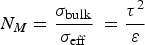
MacMullin number

Pressure

Partial pressure of fuel at the gas inlet

Effective heat flux

Ideal gas constant

Mean square displacement

r_P

Mean pore radius

Temperature

Time

V _phase

Volume fraction of analysed phase

Mass fraction

Mole fraction

x _PDF

Location of a species in the particle distribution function

Symbols

Bruggeman exponent

α _PDF

Direction of movement of a species in the particle distribution function

Scaling factor

Constrictivity

Porosity

Diffusibility or effective relative diffusivity

Tortuosity factor

κ _geo

Geometric-based characteristic tortuosity factors

κ _CFD

Flux-based characteristic tortuosity factors

λ _bulk

Bulk thermal conductivity

Dynamic viscosity

σ _bulk

Bulk conductivity

σ _eff

Effective conductivity

Tortuosity

τ_C

Characteristic tortuosity

Collision term of a species in the particle distribution function

Introduction

Electrochemical devices, including fuel cells and batteries, will play an increasing role in our lives, particularly as we transition to a low-carbon economy. However, in order to accelerate their commercialisation across a range of applications, an improved understanding of the underlying material characteristics is required. The importance of the effect of microstructure on the performance of electrochemical devices has been widely demonstrated [1], which is why studies of microstructural analysis techniques [2] are crucial for optimising vital parameters. Among these parameters, tortuosity plays an essential role in mass transport and concentration polarisation resistance [3,4]. Yet, calculating the tortuosity is not trivial, which is why a wealth of tortuosity calculation methods have been developed, not only in the electrochemical community, but also across many fields of research (optics, magnetism, geology, medicine, etc.), each with associated definitions and areas of application [5,6].

The microstructure of porous electrode and support layers in electrochemical devices is a major contributor to performance losses, especially in mass transport limiting operating regimes. This is valid for batteries, fuel cells, super-capacitors and oxygen transport membranes alike, where tortuosity is used to relate the effective transport properties of diffusion and electric or ionic flux, to its respective bulk property. As such, tortuosity is an indispensable parameter in modelling and quantifying fuel cell [7] and battery behaviour [8]. In addition, tortuosity serves as an input parameter in Newman-type models of battery performance [9] and the Adler-Lane-Steele model for electrode kinetics [10].

Owing to the importance of tortuosity for electrochemical devices, and the multitude of calculation approaches, this article reviews the use of tortuosity and various tortuosity calculation methods in the field of electrochemistry. These methods can differ considerably from each other in terms of calculation approach and data preparation techniques. Here, we deal with each in turn.

Definition of tortuosity

In geometrical terms, tortuosity τ is defined as the fraction of the shortest pathway through a porous structure Δl and the Euclidean distance between the starting and end point of that pathway Δx, illustrated in Figure 1 and equation (1). As such, τ always amounts to a value equal to or greater than unity.(1)

Figure 1.

Illustration of a tortuous path of length Δl through a porous microstructure of thickness Δx, where the shortest tortuous path is used to calculate the tortuosity of the sample.

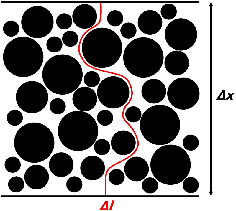
In general, when analysing a porous structure, there exists only one shortest pathway and one tortuosity value. From this geometric perspective, constrictions or bottlenecks of the pore structure are not considered. The concept of tortuosity has been adopted in a variety of sciences [5,6], such as gaseous mass transport and electronic and ionic conductivity through porous, functional layers. In these fields, tortuosity is applied in a broader way than just a simple geometric measure of the shortest path length; tortuosity is also used to quantify and describe the resistance of a structure to a flux. In this respect, the difference between ‘tortuosity’ and ‘tortuosity factor’ was coined by Epstein in 1989 [11], who used a capillary model to show that the tortuosity τ is the square root of the tortuosity factor κ, as presented in Eq. (2).

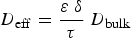
The tortuosity factor accounts for both the additional path length and its change in the velocity of a species when migrating through a porous structure. Epstein then applied this derivation in the field of diffusion, where the tortuosity factor is used to calculate the effective diffusion coefficient D _eff based on the bulk diffusion coefficient D_bulk , shown in Eq. (3), which is also valid for ionic and electronic conductivities. The nomenclature distinguishing between κ and τ is adopted in this review, and values are converted accordingly, where necessary.(2) (3) (4)

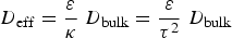
Yet, the theory behind the tortuosity factor is controversial, especially in the field of diffusive mass transport: van Brakel and Heertjes [12], for example, defined a constrictivity factor δ to account for the variation in pore diameter along the diffusion pathway, which is included in calculating the effective transport property via Eq. (4).

This constrictivity factor was later adopted by Holzer et al. [13] who stated that the implementation of τ² was used to explain high values of experimentally derived tortuosities. Consequently, the authors differentiated between two types of tortuosity: [13,14]

That, which is acquired by indirect calculations based on experimental data τ _exp.

And that, which is determined via geometric algorithms from reconstructed 3D volumes τ _geo.

Additionally, when analysing diffusive mass transport problems, depending on the diffusion mechanism taking place through a porous medium (ordinary, Knudsen and/or viscous diffusion) [15] and on the gases involved [16], different tortuosity values may dominate.

The geometric definition of tortuosity clearly suggests that there exists only one shortest pathway through a porous membrane. Yet, this pathway might not be the predominant diffusion pathway of gases and does not account for constrictive pores; not all molecules will be affected by the microstructure to the same extent when migrating through such a layer. The inherent difference of the mean free path between each gaseous species leads to different Knudsen numbers and thus, different diffusion pathways for different species at different temperatures, gas compositions and transport regimes. It can thus be inferred that, for each species and each transport regime, a different tortuosity value is dominating.

Moreover, in experimental approaches, tortuosity is not always presented explicitly, but is rather combined with porosity into a ‘diffusibility’ [17,18] or ‘effective relative diffusivity’ [19,20] value expressed as . Additionally, in the field of battery research, tortuosity is contained in the MacMullin number N_M , which relates the bulk conductivity of the electrolyte σ_bulk to the effective conductivity of the porous electrolyte σ_eff [21–24].(5)

These different definitions and applications of tortuosity cause differences in its interpretation and calculation approach. For example, geometric-based tortuosity takes only the shortest path length into account, while flux-based values rather account for the path of least resistance. Hence, the resulting values differ appreciably. These discrepancies are reflected by the vast number of different tortuosity calculation approaches shown here.

Porosity–tortuosity relationships

Employing a porosity–tortuosity relationship is one of the most fundamental and straightforward approaches to derive a tortuosity (or effective medium property) of a porous structure. Such relationships, of theoretical or empirical origin, directly calculate a tortuosity value solely based on a porosity of a sample.

In the comprehensive work by Shen and Chen [25], a review of past and present correlations is provided, among which the Bruggeman equation is the most well-known and most widespread relation in the field of electrochemistry [26]. Eq. (6) presents the generally used form of the Bruggeman relationship, where α is the Bruggeman exponent which, in its standard form, is considered to be 1.5. Recently, the authors have provided a translation and explanation of the mathematical formulation of Bruggeman which is used to derive the widely used model [27].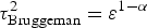(6)

While the history of the Bruggeman correlation can be traced back to the 1930s, its proliferation was not notable until the 1950s: Hoogschagen was one of the first to use the Bruggeman and Maxwell relation (cf. Eq. (7)) to validate experiments, where gas diffusion through glass spheres was measured. He observed that values for the labyrinth factor ( ) lay between the Maxwell and Bruggeman correlation, but slightly closer to the latter [17].(7)

De La Rue and Tobias achieved similar results when measuring the effective conductivity values of liquid ZnBr₂ electrolyte solution. A variety of non-conducting glass spheres of different sizes were embedded into the electrolyte to achieve different volume fractions. The conductivity as a function of volume fraction of the embedded phase was evaluated. As was the case in Hoogschagen’s publication [17], results lay between the Maxwell [28,29] and Bruggeman relation [30]. Since then, the Bruggeman equation has become a commonly used method to derive effective medium properties of porous structures in batteries [31–35] and proton exchange membrane (PEM) fuel cells [36–45]. Moreover, it has been implemented as a standard addition to predicting microstructures in electrochemistry models, such as in the COMSOL Multiphysics modelling software (COMSOL, Inc.) [24].

However, the predictions given by the Bruggeman correlation are not always consistent with experimental results [24,46]. As a consequence, researchers have adjusted the Bruggeman equation by altering the exponent α to fit experimental values. Thorat et al. [47]. even included an additional scaling factor γ to correlate the Bruggeman model with their experiments, resulting in Eq. (6) to be extended to the following form:(8)

Thorat et al. used AC impedance spectroscopy and the polarisation-interrupt method (cf. section ‘Electrochemical experiments’) to extract the tortuosity of a battery separator (Celgard 2400) and cathode samples (LiFePO₄ and LiCoO₂). Tortuosity values of the battery cathode samples were plotted as a function of porosity, and an exponential fitting curve was superimposed. The exponent of the fitting curve amounted to −0.53, which is equivalent to a Bruggeman exponent of 1.53 and thus, very close to its derived value. However, achieved tortuosities were almost twice as high as predicted by the standard Bruggeman relationship, which is why a scaling parameter γ amounting to 1.8 was introduced. This approach of adjusting α and γ was widely adopted, showing that depending on the analysed structure, both parameters can deviate from the ideal values of 1 and 1.5, respectively [32,47–55].

A further refinement of this approach was realised by Zacharias et al. [53], who made α and γ a function of their battery electrode composition. For this, the dry weight fractions of graphite, carbon black and polyvinylidene fluoride were considered, resulting in higher γ values (2.5 and 2.6) and lower α values (1.27 and 1.28) compared to values from Thorat et al. [47].

Table 1 and Figure 2 compare several derived Bruggeman exponents and scaling parameters for different porous materials for battery applications. These were each extracted as a function of several experimental measurement points and used to extrapolate the presented curves as function of porosity. It is notable that even for this small class of materials, values for α and γ differ significantly from each other. The differences in manufacturing techniques, and also the differences of composition, pore size distribution and other microstructural characteristics of each battery layer, contribute to such a large spread of values. Some of these derivations, however, achieve tortuosity values below unity when extrapolated to high porosity values, which is in contradiction to the definition and physical significance of τ. Moreover, a porosity of 100% necessitates a tortuosity of unity, yet, this is not achieved by all correlations. Both of these findings cast doubts on the usefulness of this method. As a consequence, the application and interpretation of α and γ values have to be analysed with caution.

Figure 2.

Comparison of Bruggeman exponents and scaling parameters for different battery layers referenced in Table 1.

Table 1.

Comparison of Bruggeman exponent and scaling parameter for battery layers fitted to experimental results.

Material	γ	α	Reference
Battery electrode LiMn₂O₄	1	3.3	Doyle et al. [48]
Battery separator PVdF	1	4.5	Doyle et al. [48]
Battery separator PVdF	1	2.4	Arora et al. [32]
Battery electrode MCMB 2528 and LiMn₂O₄	1	5.2	Arora et al. [32]
Battery electrode LiFePO₄ and LiCoO₂	1.8	1.53	Thorat et al. [47]
Battery graphite electrode	0.115	3.2111	Kehrwald et al. [51]
Battery graphite electrode	0.1146	3.159	Kehrwald et al. [51]
Battery electrode LiCoO₂	2.5	1.27	Zacharias et al. [53]
Battery electrode LiCoO₂	2.6	1.28	Zacharias et al. [53]
Battery separator Celgard 2400	0.667	2.43	Cannarella et al. [52]
Battery separator Celgard 3501	0.58	3.33	Cannarella et al. [52]
Battery separator GMB 500 mAh	1.77	1.77	Cannarella et al. [52]

Hence, evaluating the validity of the Bruggeman correlation is still an ongoing field of research. Chung et al. [56] used X-ray computed tomography and simulation techniques for an extensive study to evaluate the effect of battery membrane fabrication and processing methods on the tortuosity. In total, 16 LiNi_1/3Mn_1/3Co_1/3O₂ battery electrodes with varying weight ratios were manufactured and reconstructed using X-ray synchrotron tomography [57]. Tortuosity was then extracted by simulating mass transport according to Fick’s law across the sample volume (see section ‘Flux based algorithms’). It was shown that calculated tortuosity values always lie slightly above the Bruggeman correlation. For further investigation, samples based on the particle size distributions of the imaged samples were computer generated, for which the orientation and particle packing was varied. It was discovered that perfectly ordered particle distributions result in tortuosities close to the Bruggeman relationship throughout the range of porosity values [56].

Continuing work in the field of battery research from Wood and co-workers (cf. [54,56,57]) culminated in the development of an open source programme called BruggemanEstimator [58]. This programme allows the extraction of the Bruggeman exponent α in each dimension of a 3D sample volume using two 2D images, namely one top view and one cross-sectional view. The Bruggeman exponent of the sample is achieved by applying the differential effective medium approximation method introduced by Bruggeman. In comparison to previously obtained values, the results calculated by the BruggemanEstimator software agreed well with numerical tortuosity calculation methods [58] and have been recently applied in practice [59]. This approach is similar to stereological methods which quantify 3D properties based in 2D image slices [60]. The advantage of stereology is the reduced experimental efforts necessary to extract results. However, Taiwo et al. [2] recently concluded that values based on stereological approaches may deviate appreciably from 3D measurements.

Moreover, a wide range of recent studies report conflicting results on the validity of the Bruggeman correlation when compared to the calculations done using tomography techniques. Conclusions vary substantially as in some instances, simulations agree well with the Bruggeman correlation [34,56], while considerable disagreement was observed in other cases [45,61–63]. The reason for this seems to be sample specific, as heterogeneity and geometry are characteristics of porous materials that are not accounted for by the Bruggeman correlation. The aforementioned studies have shown that the characteristic shape of the analysed microstructure has considerable effects on the validity of the Bruggeman relation: spherical structures, which follow Bruggeman’s initial hypothesis very closely, adhere to the correlation. The correlation, however, is less suitable for connected solid phases and complex porous networks.

This is further complicated by the distinctions (or lack thereof) between geometrical and transport limiting tortuosity [64]. Moreover, porosity–tortuosity relationships provide limited information in areas, where the analysed sample consists of several layers with different microstructural features, such as multi-layer battery separators [52]. These combine different properties into a single separator; i.e. each individual layer exhibits distinct structural properties, and for this reason, the simplified assumption of a homogenous sample volume made by the Bruggeman correlation is no longer valid. As a conclusion, it can be stated that porosity–tortuosity relationships are only applicable and reliable when executed across homogeneous microstructures which are similar to the microstructure used to derive the respective relationship.

Experimentally derived tortuosity

Historically, the lack of detailed geometrical information on complex porous media in 3D has limited the ability of researchers to extract meaningful data on the tortuosity of a porous body. In the absence of this information, effective transport properties of porous structures have been derived experimentally by means of diffusion cell experiments [17,18,65–71] and electrochemical measurements [16,20,47,72].

Diffusion cell experiments

As reviewed by He et al. [73], diffusion measurement methods in the field of fuel cell research aim at extracting effective diffusion coefficients for distinct gas mixtures. Typically, a porous sample is mounted between an upper and a lower gas channel where two different gases enter the upper and lower chamber. Owing to the concentration gradient across the porous material, diffusion of either gas to the opposite channel is induced. Measuring the concentration of either gas in both streams allows the calculation of the diffusion fluxes across the membrane via a mass balance over the cell, as illustrated in Figure 3. The effective binary diffusion coefficient and, in turn, the tortuosity of the sample, are subsequently derived by applying a suitable diffusion model.

Figure 3.

Mass balance over a Wicke Kallenbach diffusion cell to extract the diffusion flow rate across a porous sample.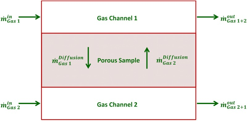

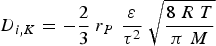
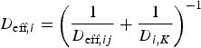
The applicability of such models is dependent on the diffusion mechanism taking place through the porous medium (ordinary, Knudsen and/or viscous diffusion cf. [15,74,75]). The most direct diffusion model considering ordinary and Knudsen diffusion is the Fick model. For this, Fick’s law is extended by combining the Knudsen diffusion coefficient D_i,K , (Eq. (9)) with the effective binary diffusion coefficient via the Bosanquet equation (Eq. (10)). Moreover, Fick’s model is capable of incorporating viscous flux via Darcy’s law, as presented by Eq. (11). In this case, the model is referred to as advective–diffusion model [76].

In the following equations, r_P is the mean pore radius, R is the ideal gas constant, T is the temperature, M is the molar mass, is the effective diffusion coefficient of a species, B_O is the viscous flow parameter and μ is the dynamic viscosity and p is the pressure and w is the mass fraction.(9) (10) (11)

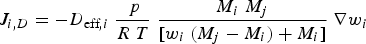
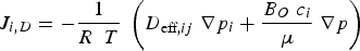
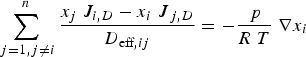
While Fick’s law assumes equimolar diffusion in a binary gas mixture, Mills [77] suggested that diffusion follows equimass principles. By converting the molar concentration gradient of Fick’s first law into a gradient of mass fraction, the governing equation for equimass diffusion was achieved:(12)

Again, the Bosanquet equation and Darcy’s law can be used to extend the formulation to cater for additional diffusion mechanisms besides ordinary diffusion. The effective diffusion coefficients are directly achieved via the above models which make their application straightforward. More complex models, such as the Dusty Gas Model (DGM) [74] or Maxwell–Stefan Model (MSM), shown in Eq. (13) and Eq. (14), respectively, combine several diffusion modes a priori. The DGM, for example, includes expressions for ordinary, Knudsen and viscous flux, where x is the molar fraction: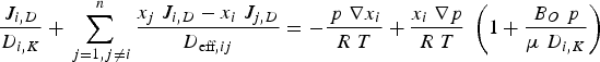(13) The MSM uses the same correlation as the DGM, but neglects Knudsen diffusion effects. As a result, coefficients related to Knudsen diffusion drop out of equation Eq. (13) and result in the following formulation:(14)

The accuracy of these models has been discussed [78] and evaluated in literature, predominantly by comparing them to measured concentration polarisation losses in SOFC anodes [79,80]. In these experiments, the DGM achieved highest accuracy among the analysed models, which might be one reason for its widespread use in literature [80–84], while the simplicity but lower accuracy of the Fick model was frequently highlighted. However, in these cases, tortuosity is usually used as a fitting parameter to tailor calculation results to measured data. Consequently, the extracted tortuosity values are highly dependent on the accuracy of the applied model.

One recent application of extracting the tortuosity of a porous sample via diffusion cell experiments was presented by Tjaden et al. [85]. In their analysis, a variety of binary gas mixtures were tested on a planar YSZ porous support layer of an oxygen transport membrane. It was shown that the tortuosity for different binary gas mixtures is not a constant value, but depends on the involved gaseous species. Owing to the difference in mean free path between the different constituents, different diffusion pathways dominate and thus, different tortuosity values are achieved. For example, at ambient temperature, tortuosity based on the diffusive flux of CH₄ in the CH₄–N₂ binary gas mixture amounted to approximately 2.3, while tortuosity of the N₂ diffusion flux amounted to approximately 2.5. In addition, the authors showed that tortuosity increased with increasing temperature: the average tortuosity of all binary gas mixtures increased from 2.36 to 2.73.

The contrary temperature-dependent behaviour of measured diffusion coefficients was observed by Zamel et al. [18]. A Loschmidt cell was used to measure the effective diffusion coefficient of a O₂–N₂ gas mixture migrating through carbon paper, which is commonly applied as the gas diffusion layer (GDL) in polymer electrolyte membrane (PEM) fuel cells. When increasing the temperature from 25°C to 80°C, the bulk diffusion coefficient of the gas mixture, achieved via a resistance network model based on Fick’s law, increased from approximately 0.2 cm²s⁻¹ to 0.275 cm²s⁻¹, while the effective diffusion coefficient increased from approximately 0.05 cm²s⁻¹ to 0.075 cm²s⁻¹. This causes the factor to increase by approximately 11.5% from 0.252 to 0.281. Thus, when considering a constant porosity value, the tortuosity decreases to the same extent. In addition, the authors compared the calculated diffusibility values to a set of porosity–tortuosity relationships, among others, the Bruggeman relation. In all cases, these relationships overestimate the effective diffusion coefficient (and thus, underestimate tortuosity), which was also observed by Tjaden et al. [85].

The discrepancies in temperature dependence might be caused by the fundamental difference in microstructural aspects: while YSZ-based porous structures are tailored to feature connected solid phases with specific porosities, carbon paper-based gas diffusion layers are an accumulation of randomly oriented, fine fibres, typically with much higher porosity. The resulting differences in pore size distribution, mean pore diameter and porosity cause the observed diffusion mechanisms to differ significantly among such samples.

Electrochemical experiments

Mass transport limitations play a vital role in electrochemical devices as they are responsible for concentration polarisation at high current densities. For example, as current densities increase, the fuel demand in a fuel cell increases linearly, as shown in Eq. (15), where is the molar flow rate of fuel gas, i is the current density, A is the area, n is the equivalent electrons per mole of reactant and F is the Faraday constant: [7](15)

The fuel consumption rates at the active sites of a fuel cell are limited by the maximum diffusion rate of reactant through the porous structures. As introduced in previous sections, diffusive mass transport and, as such, mass transport limitations are a function of the complex microstructure of the involved porous membrane layers. Hence, microstructural parameters, such as tortuosity, are achievable by measuring concentration losses of fuel cells and applying gas diffusion theory.

In this respect, SOFCs offer the possibility to investigate the effect of fuel gas compositions on the performance owing to their wide fuel flexibility. A thorough study of this topic was presented by Jiang and Virkar [16]. As the effects of mass transport limitations are dominating under high current density operations, Jiang and Virkar modified Fick’s law to express the effective diffusion coefficient as a function of the limiting current density of the fuel cell under specific operating conditions. 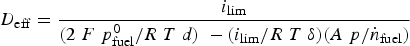The resulting equation is presented thereafter, where i_lim is the limiting current density, is the partial pressure of fuel at the gas inlet and d is the thickness:(16)

The limiting current density was measured experimentally from polarisation curves for a set of binary and ternary fuel gas mixtures, including H₂-H₂O, CO-CO₂, H₂-He-H₂O, H₂-N₂-H₂O and H₂-CO₂-H₂O, each under varying concentrations. Tortuosity values were then calculated by reversing the Bosanquet equation shown in Eq. (10). At 800°C, the lowest tortuosity values were achieved for the H₂-H₂O mixture, which, on average, amounted to 2.23, while the highest tortuosity values were calculated for the H₂-CO₂-H₂O mixture, amounting to 2.73. Moreover, in direct comparison between the two binary gas mixtures, it was revealed that fuel cell performance was higher using H₂ as fuel gas rather than CO which, besides the lower electrochemical activity of CO, was due to the significantly faster diffusion rate of H₂. These results confirm the findings of different tortuosity values for different binary gas mixtures presented in the previous chapter.

Brus et al. [72] adopted the same methodology to compare electrochemically derived tortuosity values with an image-based tortuosity calculation method, namely the random walk method (cf. section ‘Voxel-based calculation methods’). For their experiments, a button-type SOFC sample was manufactured to measure impedance spectra and polarisation characteristics at 700°C and 800°C. This way, the limiting current densities were extracted for H₂ concentrations between 2.5 and 90% in N₂ and inserted into Jiang and Virkar’s model. After these experiments, the 3D microstructure of the anode was reconstructed using focused ion beam–scanning electron microscope (FIB–SEM) tomography, and the random walk method was executed. For each hydrogen concentration and for both operating temperatures, a distinct tortuosity value is calculated, whereas the random walk method results only in a single value, as shown in Figure 4. Here, only the tortuosity values calculated for low hydrogen concentrations and, as such, high concentration polarisation were considered as accurate representative values. In these cases, the experimentally derived tortuosities agreed well with the random walk value. Hence, under standard fuel cell operating regimes, where activation and Ohmic losses dominate, concentration losses, and thus the tortuosity of the porous layers affect the performance only slightly.

Figure 4.

Comparison of experimental- and image-based tortuosity values at different temperatures and for varying H₂ concentrations in N₂ reproduced with permission from Elsevier [72].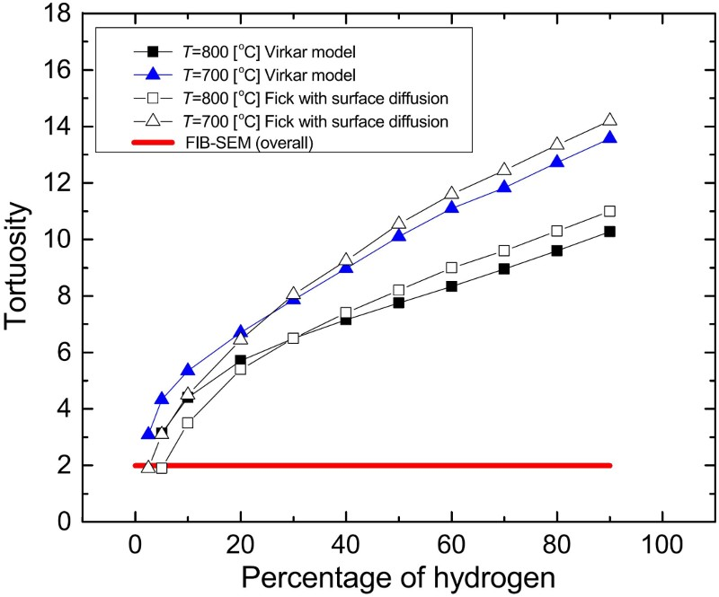

However, experimental-based tortuosity values are valid only for the specific experiment at hand. While the results between image- and experimental-based tortuosity values in the above case are close, this agreement might not be reproducible when the fuel gas composition changes.

Figure 4 also shows that higher temperatures have a positive effect on tortuosity: for each fuel gas composition, the tortuosity is lower at higher temperature, which can be explained by the higher catalytic activity and faster diffusion rate. Yet, aside of the effect of temperature, the influence of structural parameters, such as the layer thickness on the tortuosity of SOFC anodes, is of interest. This was investigated by Tsai and Schmidt [86–88], who, again, applied Jiang and Virkar’s approach for this purpose. While they observed the same dependency of tortuosity on H₂ concentration as Brus et al. [72], Tsai and Schmidt [88] showed that electrode thickness had no effect on the achieved tortuosity values, which is expected for steady state operation.

Electrochemical experiments have also been applied to study microstructures of lithium-ion battery materials. Thorat et al. [47] used polarisation-interrupt (or restricted diffusion) experiments [89–91] and impedance spectroscopy to measure the tortuosity in electrode and separator layers. Using the polarisation interrupt technique, Thorat et al. derived the tortuosity of two distinct active material films consisting of LiFePO₄ and LiCoO₂, respectively. On the other hand, AC impedance spectroscopy was carried out to determine the effective conductivity of the electrolyte in the separator and ultimately, the MacMullin number or the tortuosity of the separator itself. While the authors used the AC impedance experiments to validate the polarisation interrupt experiments, the effect of porosity on the tortuosity of the active material films was in the centre of their research and led to the adjustment of the scaling factor to 1.8 and Bruggeman exponent α to 1.53 [47] as discussed in section ‘Porosity-tortuosity relationships’.

With the development of advanced manufacturing techniques, lithium ion battery electrode microstructures can be tailored and optimised to meet user- and application-specific demands. Bae et al. [92], for example, applied a two-pronged approach to improve electrode design: first, using a modified model by Doyle and Newman [93], the tortuosity of different electrode microstructures with periodically spaced flow channels was calculated. Based on these results, LiCoO₂ electrodes mimicking the modelled microstructures were manufactured using a co-extrusion procedure. In their model, electrodes with flow channel spacing equal to or smaller than the electrode thickness offered lowest tortuosity values. To validate these findings, charge and discharge curves of the manufactured samples with large, medium and small channel spacing were measured. As predicted, the sample with finest and most closely spaced channels yielded highest specific capacity of approximately 8 mAhcm⁻² at C-rates of one and two. The authors attributed this improved capacity to the lower tortuosity of their manufactured electrode, validating their model.

In general, experimental set-ups can be adjusted to fit the operating conditions of the analysed specimen. However, as the derived results are fitting parameters, the tortuosity values are highly dependent on the applied model. Moreover, while fuel cell experiments can be highly versatile in terms of operating temperature and applied fuel gas, batteries are not subject to such variations. Hence, it appears to be easier to extract an overall valid tortuosity value for a battery layer than a fuel cell layer.

Tortuosity calculation in 3D volumes

The advent of sophisticated and easily accessible tomography methods has increased the amount of obtainable data of porous samples which fundamentally changed the perception of microstructural characterisation in 3D [94]. FIB-SEM slice and view tomography [95], and X-ray computed tomography (X-ray CT) [96, 97] are among the most prominent methods of reconstructing a sample in three dimensions. Even though the operation and image acquisition of both methods are radically different, comparative studies showed that acquired data are identical when the resolution is the same [85, 98, 99].

FIB-SEM tomography is commonly used in SOFC research to achieve solid phase segmentation between the YSZ and Ni-phase in the anode [100]. Moreover, this technique offers the possibly of using additional analysis methods, such as energy dispersive spectroscopy, electron backscatter diffraction and secondary ion mass spectroscopy [1]. Hence, 3D chemical and crystallographic data can be acquired in parallel with microstructural parameters. The advantage of X-ray tomography lies in the non-destructive nature of operation which allows in-situ and in-operando analyses. Changes in microstructure as function of continuing and varying operating conditions can be tracked [101]. This allows a four-dimensional analysis of microstructural evolution during processing, redox reactions and degradation [1].

In recent years, tomographic reconstruction of microstructures in electrochemical devices, illustrated in Figure 5, has become increasingly widespread, offering the possibility to evaluate vital parameters, such as triple phase boundary length in SOFCs [102, 103], connectivity [104], phase distribution [105] and tortuosity [81, 102] at different length scales [106]. Additionally, the effect of microstructural parameters on the performance of electrochemical devices has been evaluated by generating synthetic 3D volumes in silico [34, 56, 107, 108]. The purpose for this process is to directly evaluate the effect of specific microstructural variations, such as porosity, pore size distribution, shape or packing orientation of particles on mass transport.

Figure 5.

Illustration demonstrating that high-resolution tomography is necessary to extract microstructural features which affect diffusive mass transport.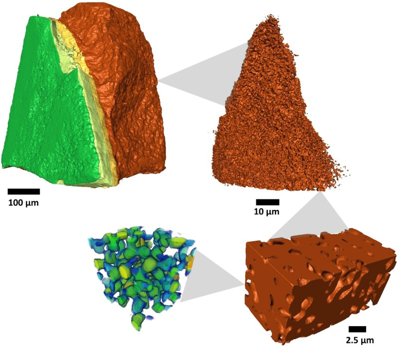

There remains some confusion in the literature regarding the different definitions of tortuosity for the purpose of image-based modelling: here, we distinguish between two main approaches in extracting tortuosity:

Geometric-based algorithms, which aim to determine the shortest path length through a porous structure by purely considering geometric aspects.

Flux-based algorithms, which mimic mass transport and diffusion behaviour, which is not taken into consideration in geometric-based algorithms. These methods are further divided into the following two subsections:

Voxel-based algorithms that take the extracted dataset and directly execute tortuosity extraction techniques across the voxel domain of the analysed phase.

Mesh-based approaches which rely on generating a volume mesh of the analysed phase to prepare the sample for computational fluid dynamics (CFD) programmes.

It is evident that the increase in the development of such techniques correlates with the increasing accessibility of tomography equipment and high-performance computers.

Geometric-based algorithms

Geometric algorithms are commonly used to find the shortest pathway through a porous structure and thus, its tortuosity. The pore centroid method [63, 106, 109–111], the fast marching method (FMM) [2, 112, 113], the distance propagation method [114], as well as or other shortest path search methods [115, 116] achieve this by being executed on the voxel domain of the analysed phase. These methods are straightforward in their application, as mesh preparation and refinement is not required. In addition, the results directly follow the initial definition of tortuosity, making them conceptually easier to interpret. Furthermore, apart from the pore centroid method, these algorithms create a distance map, which incorporates the distance of each pixel to the starting plane of the algorithm. Using the resulting distance map allows not only the identification of the shortest pathway, but also the generation of a tortuosity histogram.

The FMM achieves this by simulating an advancing front, starting from one plane of the sample towards the opposite plane in the considered phase. The algorithm measures the time it takes for the front to reach each pixel on its way. By knowing the speed of advance of the front and the time it takes to arrive at a pixel, the distance between each pixel and the starting plane is achieved and tabulated in a distance map. Finally, tortuosity is calculated by dividing the shortest path length between two opposing planes by the Euclidean distance of the two endpoints of that path.

Jørgensen et al. [112] exploited the FMM-based tortuosity histograms of a strontium-substituted lanthanum cobaltite (LSC) and gadolinium-substituted ceria (CGO) SOFC cathode to understand microstructural characteristics of each phase. In accordance with each phase’s volume fraction, LSC features higher tortuosity values than CGO. The distinct shapes and specifics of each phase’s tortuosity achieved by the FMM-based histograms are able to provide more insight into the microstructural build-up of a sample compared to a single, mean tortuosity value.

Yet, tortuosity histograms do not show where the specific high or low tortuosity values are located within the sample. This was realised by Chen-Wiegart et al. [114], who combined different tomography methods and distance propagation-based tortuosity calculation approaches on various samples. Specimens included, among others, a LiCoO₂ battery cathode, which was reconstructed using an X-ray tomography. Geometric tortuosity values were then achieved by pixel counting and distance-measuring techniques. The resulting values were presented as 3D distribution across the battery cathode sample, as shown in Figure 6. The local variation in the image slices ranges from 1 to 2.5, which can also be ascertained from the tortuosity histogram. However, as tortuosity poses a resistance to mass and charge transport, the local tortuosity distribution is capable of pinpointing areas of low reactivity. It can be used to explain regions of increased charge transfer, areas of low fuel conversion, uneven charging or catalyst utilisation and degradation. Shearing et al. [115] extended the approach of spatial distribution of geometric tortuosity to include additional characteristics such as volume specific surface area and porosity. A reconstructed graphite Li-ion battery electrode was segmented into a mosaic of equally sized volumes and for each tile, the aforementioned parameters were calculated and visualised to highlight the relation between them. While in most cases, tiles with high porosity featured low tortuosity, some sub-volumes exhibited low tortuosity coupled with low porosity. Even though this combination seems counterintuitive, it emphasises the complex interrelation between different microstructural parameters which are not always as clear as expected.

Figure 6.

Geometric tortuosity distribution of the pore phase of the LiCoO₂ battery cathode of yz (A), xz (B) and xy (C) planes reproduced with permission from Elsevier [114].

For comparative purposes, Chen-Wiegart et al. executed a diffusion simulation analogous to the one used in [4] (cf. section ‘Mesh-based calculation methods’) across the same sample volumes. It was shown that the results between the distance propagation and diffusion method of the pore phase in the LiCoO₂ sample agreed well. However, when applying the same calculation approaches to two SOFC samples, the geometrically derived tortuosity values for the pore and YSZ phases were consistently below the diffusion-based tortuosity methods. The difference might stem from the inherent difference between geometric- and diffusion-based considerations: the geometrically shortest path through a structure is not always the path of least resistance for a flux, owing to the presence of constrictions and pore necks. Further discussion on the differences of these considerations is presented in section ‘Flux-based algorithms’.

In contrast to the aforementioned algorithms, the pore centroid method does not provide a histogram of tortuosity values or spatial distribution of tortuosity, but rather arrives at one specific value of tortuosity along each dimension of a sample. The calculation algorithm follows the centre of mass of a phase of a 2D plane along the third axis of the volume. The length of the pathway going through each centroid is then calculated and used to determine the tortuosity as depicted in Figure 7. Despite its shortcomings in comparison with the previous algorithms, the pore centroid is a standard option in image and volume processing programmes such as Amira and Avizo (both FEI). As such, it is easily applied for comparative studies and capable of giving a quick tortuosity estimate.

Figure 7.

Illustration of the pore centroid method calculation approach which measures the distance d_(n) of the centres of mass between two 2D image slices.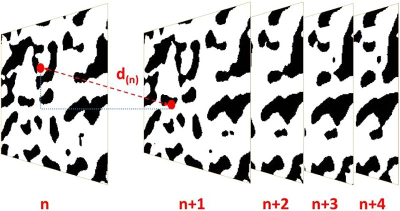

Cooper et al. used the pore centroid method for comparison reasons when studying an SOFC [111] and a battery electrode (cf. section ‘Mesh-based calculation methods’) [63]. In [111], the tortuosity of the solid and pore phase of an LSCF SOFC cathode was determined by a variety of calculation algorithms, namely heat flux simulation (cf. section ‘Mesh-based calculation methods’), Avizo XLab plugin, diffusion simulation, random walk method (cf. section ‘Voxel-based calculation methods’) and pore centroid method. These algorithms were executed across the same sample after imaging at 14°C and 695°C using synchrotron X-ray nano CT which have previously been extracted by Shearing et al. [117]. The pore centroid method produced the lowest tortuosity values for both phases at both temperatures and closely followed the Bruggeman relationship. Yet, the flux-based calculation algorithms agreed well with each other as values lay between the heat flux simulation and the random walk method. The average tortuosity for the pore phase amounted to approximately 1.21 in all three dimensions at both temperatures and lay visibly below the values reported by Gostovic et al. [109] using the same method. Large variability in homogeneity of a sample significantly affects the results achieved by the pore centroid method, causing visible fluctuations. In this respect, Cooper [118] pointed out that if the analysed characteristic feature becomes small compared to the control volume, the centroid of each 2D plane will tend towards the centre, resulting in a tortuosity of unity which casts doubt on the applicability of this approach.

Flux-based algorithms

Even though geometric-based tortuosity calculation algorithms can extract useful data concerning the distribution of geometric tortuosity across a sample, these algorithms do not mimic the flux-like behaviour of transport phenomena. For example, small connections consisting only of one voxel would contribute only a negligible amount to the overall flux of transported species, while they are fully included in the above calculation methods. As a result, flux-based algorithms focus on simulating the transport mechanism at hand to extract the tortuosity of a sample. Here, this method is separated into two parts, namely voxel- and mesh-based calculation approaches.

Voxel-based calculation methods

Voxel-based algorithms are directly executed across the voxel domain of the reconstructed volume. This means that for the methods introduced below, no additional re-tessellation or re-meshing steps are necessary after the sample has been segmented. In most cases, a binarised 2D image sequence is sufficient to operate the calculation procedure.

One of the first applications of combining X-ray nano tomography with image-based tortuosity calculation was presented by Izzo et al. [81], where X-ray CT was used to gather microstructural parameters of a porous SOFC anode, including porosity, tortuosity and pore size distribution. The authors solved the Laplace equation of diffusive mass transport through the pore phase of the electrode as explained in a different publication from the group [119]. Grew et al. [120] applied the same methodology, but extended its application to the solid phases of a Ni-YSZ SOFC anode. As effective ionic conductivity and electronic conductivity are affected by the tortuous nature of fuel cell electrode layers (cf. equation 3), tortuosities of solid phases are equally as important as of pore phases. Yet, they were at least a factor of 1.2 higher.

Their work was further refined in [121] by calculating the representative volume element (RVE) of the pore phase tortuosity by solving the Laplace equation using the same method. Cooper [118] programmed a MATLAB (Mathworks) Laplace solver called TauFactor [122–^[123] 124] to extract the tortuosity of a two-phase segmented 3D tiff stack as shown in Figure 8. The solver then determines the tortuosity in each dimension for both phases. In [118], Cooper compared the results of the TauFactor solver to previous work presented in [111], revealing that the solver gives similar results as the Avizo package XLab Thermo and the heat flux simulation.

Figure 8.

Results of the TauFactor solver by Cooper [118] running across the pore phase of a porous sample showing the binary image map, the initial, linear concentration distribution and the concentration distribution at steady state.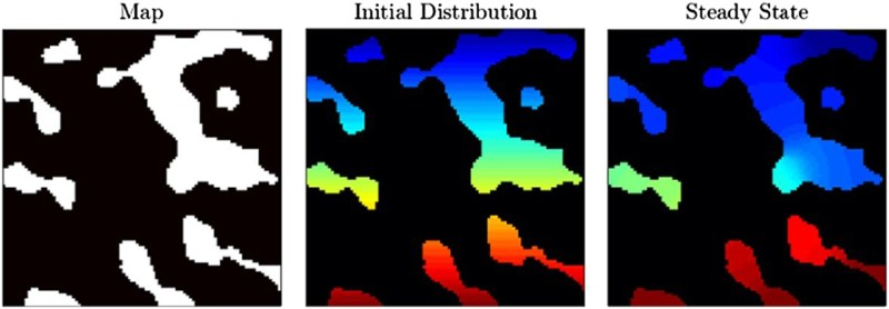

Aside from solving the Laplace equation to arrive at the tortuosity of their sample, Izzo et al. [81] included the lattice Boltzmann method (LBM) [125] to model multi-component gas transport coupled with an electrochemical model to visualise the H₂ distribution in the anode. Owing to the capability to model gaseous, ionic and electronic transport, the LBM became widely applied in fuel cell research, also with the focus of extracting tortuosity in different phases of a functional layer [103, 126–^{[127]
[128]
[129]
[130]} 131]. For this, the LBM uses the particle distribution function (PDF) , which is a function describing the probability of encountering a particle of a species i at a certain location x_PDF with a certain speed at a certain point of time t moving in a certain direction α_PDF .

The LBM consists of two steps, namely streaming and collision, which are carried out on each point of a lattice: during streaming, the particles migrate to adjacent lattice points while during collision, the interactions between particles at each lattice point governed by the collision term are computed. Both steps are collectively expressed by the lattice Boltzmann equation: [119, 132](17)

Using this approach, Iwai et al. [103] arrived at tortuosity values for each phase in the porous Ni-YSZ anode by calculating the effective diffusion coefficient and effective ionic as well as electronic conductivities of the respective phases. The anode sample was reconstructed based on FIB-SEM tomography, where the Ni and YSZ phases were identified via EDX mapping, to correlate the correct phase to the respective electron image. Table 2 compares the achieved tortuosity values for all three phases along each dimension using the LBM as well as the random walk method, which is introduced thereafter. It is evident that the tortuosity values of the solid phases are higher compared to those of the pore phase, which is identical to the findings presented by Chen-Wiegart et al. [114] using a distance mapping approach. Nevertheless, values for the pore phase tortuosity are lower than but comparable to the values found by Izzo et al. [81] However, owing to the observed directional anisotropy of the solid phase tortuosities, Iwai et al. concluded that the sample volume was not sufficiently large to present effective ionic and electronic conductivity values. Vivet et al. [133] achieved similarly high Ni-phase tortuosity values using a finite difference method. However, owing to the higher YSZ fraction in their sample, achieved YSZ tortuosities lay below the values reported by Iwai et al. [103].

Table 2.

Tortuosity values for pore, Ni and YSZ phase of an SOFC anode calculated using the random walk method and LBM [103].

		Random walk method	Lattice Boltzmann method
Pore phase	x	1.43	1.42
	y	1.41	1.44
	z	1.33	1.35
Nickel phase	x	4.70	4.66
	y	5.43	5.43
	z	2.63	2.63
YSZ phase	x	5.28	5.26
	y	3.87	3.85
	z	3.14	3.14

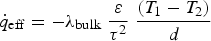
The aforementioned random walk method [29, 103, 134–137] mimics a diffusion process by distributing a number of non-sorbing particles, so-called walkers, across the segmented voxel phase. The algorithm then starts a time-step sequence, where at each step, every walker choses one neighbouring voxel as its next location. If that neighbouring voxel is of the same phase (e.g. pore phase), the walker migrates to that new location. However, if the chosen neighbouring voxel is of a different phase (e.g. solid phase), the walker remains at its current location and chooses a different neighbouring voxel at the following time step. By repeating this sequence, the mean square displacement of the walkers in the analysed phase is calculated which, in turn, is used to achieve an effective diffusion coefficient D _eff, where V _phase is the volume fraction of the analysed phase:(18)

Tortuosity is then calculated by comparing the effective diffusion coefficient to the bulk diffusion coefficient through an empty volume of equal dimensions. The random walk approach was first formulated in the 1990s [5, 138, 139] and found its way into electrochemistry via Kishimoto et al.[134], after having been used to extract the tortuosity of porous rocks [140]. However, the obtained tortuosity is affected by the number of walkers and by the number of time steps chosen for the calculation. This is why, in [103], 100,000 walkers and 10,000,000 time steps are chosen to ensure high accuracy of the results (cf. Table 2).

A similar comparative study using the random walk method was carried out by Tariq et al. [137]. The tortuosity values of a Li-ion battery anode, calculated by the random walk method, were compared to the results based on a sub-grid scale finite volume method explained by Kishimoto et al. [141]. As shown in Table 3, results for both methods agree excellently, revealing a higher tortuosity along the z-axis of the pore phase. The authors noted that a RVE analysis would reveal, if this anisotropy was persistent or if the high value was caused by a local heterogeneity. Yet, it was explained that the computation time needed for the random walk method is only a fraction compared to the finite volume method.

Table 3.

Tortuosity values for graphite and pore phase using the random walk method and finite volume method [137].

		Random walk method	Finite volume method
Graphite phase	x	1.57	1.56
	y	1.92	1.89
	z	2.59	2.57
Pore phase	x	1.42	1.42
	y	1.19	1.18
	z	2.39	2.37

Mesh-based calculation methods

By applying the same tomography methods mentioned in the previous section, extracted datasets can be represented as volume meshes for additional analysis algorithms enabled, for example, by CFD or finite element software packages. These programmes allow the simulation of heat, mass and/or charge transport through the generated mesh of the investigated structure to subsequently evaluate the tortuosity. In the data preparation process, parameters chosen for sample smoothing, surface repair and mesh generation affect mesh quality and thus the simulation results. Hence, care must be taken when choosing these parameters [85] and sensitivity analyses should be carried out to verify the consistency of the chosen values.

Pioneering work in this field was realised by Wilson et al. [102], who reconstructed an SOFC anode using FIB-SEM tomography. The tortuosity of the pore phase was then extracted to assess the mass transport limitations at high current densities. For this, the sample volume was converted into a finite element mesh to solve the Laplace equation in FEMLAB (now COMSOL Multiphysics).

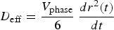
Extensive simulation work in the field of electrochemical devices, using a similar approach as presented above, has been carried out by Ivers-Tiffée and co-workers: initially based on COMSOL Multiphysics, the group developed the 3D finite element tool ParCell3D to model the behaviour of fuel cells [142–145] and batteries [146]. Joos et al. [147] used this tool to investigate the RVE of tortuosity of an SOFC cathode for both phases, namely the pore and the mixed ionic-electronic conducting LSCF phase. In total, the RVE of porosity, volume-specific surface area and tortuosity were calculated for three separate volumes, of which the latter one is presented in Figure 9. The results for both phases in sample volumes 1 and 3 agree excellently with each other, achieving a flat development for electrode thicknesses of l_cat > 10 μm. However, the tortuosity of the LSCF phase in sample two takes an electrode thickness almost twice as long as for the other sample volumes to produce a flat curve. To follow the nomenclature of this review, it has to be pointed out that τ in Figure 9 ought to be replaced by τ [2].

Figure 9.

RVE analysis of the tortuosity factor for the pore and LSCF phase of an SOFC cathode as function of electrode thickness reproduced with permission from Elsevier [147].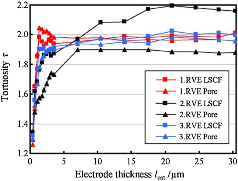

Besides COMSOL Multiphysics [148, 149], researchers have calculated tortuosity using programmes, such as Cast3M [150] or custom made models, which focus on a specific electrochemical device, such as Batts3d [34, 56, 151].

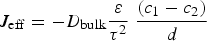
In addition to simulating mass and charge transport, the tortuosity is also computable by exploiting the mathematical similarity between Fourier’s law of heat conduction and Fick’s law of diffusion shown in Eq. (19) and Eq. (20), where J_eff is the effective diffusion flux, c is the molar concentration, is the effective heat flux, λ_bulk is the bulk thermal conductivity [85, 106, 152–154]. By rearranging the temperature gradient, the heat flux and thus, the tortuosity can be calculated along each axis of a sample. Cooper et al. [63] scanned a commercially available LiFePO₄ battery cathode using an X-ray synchrotron nano CT and investigated the tortuosity of the pore phase using heat flux simulation. A cube of 8.8 μm side length was cropped and meshed using an adaptive polyhedral volume mesh. The heat flux across the porous phase of the sample was simulated in StarCCM+ (CD-adapco), resulting in a temperature distribution across the analysed volume (see Figure 10), where the temperature of each mesh element can be understood as a concentration value of a migrating species.(19) (20)

Figure 10.

Temperature distribution across the porous phase of an YSZ porous support membrane of an oxygen transport membrane.

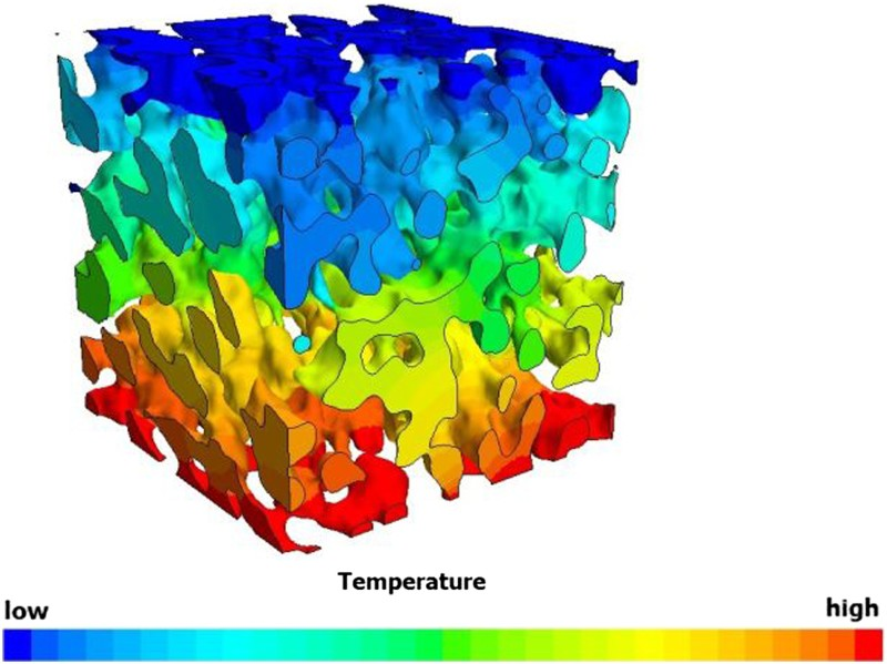
For further analysis, the sample was divided into eight non-overlapping sub-samples to compare the pore centroid and heat flux-based tortuosity factors. To extract a single tortuosity value for each sub-volume, the concept of the characteristic tortuosity τ_C was introduced: [63, 85]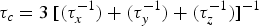(21)

The geometric-based characteristic tortuosity factors (κ _geo) were then plotted as a function of the flux-based characteristic tortuosity factors (κ _flux). The resulting graph revealed a high degree of correlation following Eq. (22). This equation reveals that the simulation-based tortuosity factor (and as such, tortuosity) is always higher than the geometric-based value of the same sample in cases where either value is >1. As mentioned previously, geometric tortuosity algorithms do not take the effect of pore constrictions into account, which would affect a transport flux. This means that any connection consisting of only one voxel in diameter is fully considered in the calculation process, while from a flux point of view, such a pore would not allow a significant amount of mass/charge to pass through. As a result, geometric-based tortuosity values tend to be visibly lower compared to simulation-based values [63, 85].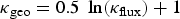(22)

It is common practice to subdivide a given sample volume into an array of smaller sub-samples and extract the tortuosity for each individually [51, 147, 155]. Although non-trivial, this approach allows researchers to extract similar results as tortuosity histograms and tortuosity distribution maps (cf. section ‘Geometric-based algorithms’) using flux-based methods. This approach reveals the homogeneity or heterogeneity of a sample, comparable to tortuosity histograms, and pinpoints the locations of high or low tortuosity. Kehrwald et al. [51] were among the first ones to apply this methodology on a battery electrode by solving Fick’s law using the programme Star-CD (CD-adapco) on a total of 12 sub-volumes. Local tortuosities showed differences of a factor of three, which might lead to inefficiencies during charging and discharging of the battery: Li⁺ ions will avoid areas with higher tortuosity, but seek areas with low tortuosity, highlighting the need for homogeneous microstructures in this field to prevent spatial distribution of performance and degradation [155]. In addition, microstructural inhomogeneities might be the cause of failure mechanisms and material fractures [51].

Summary

Table 4 and Table 5 list pore phase tortuosity factors and tortuosity values for different image-based calculation methods along all three axes of porous samples. Calculation approaches, which take flux-like behaviour into account (cf. Table 4), arrive at higher tortuosity values compared to purely geometric-based algorithms (cf. Table 5). It is thus imperative to distinguish between these two approaches as otherwise, misinterpretation may ensue. Furthermore, differences in tortuosity values are observed even when analysing the same type of samples. This can be explained by the chosen imaging resolution; higher resolution uncovers smaller pore structures and improves pore connectivity. However, the effect of varying the pixel size can differ substantially, depending on the analysed microstructural parameter. Shearing et al. [106] imaged the same commercially available Li-ion battery cathode using different X-ray systems: a laboratory-based micro CT system and a laboratory-based nano CT system. The pixel size for each system amounted to 597 and 65 nm and the extracted volumes amounted to 10,434,731 μm³ and 75,164 μm³, respectively. The authors calculated the porosity, geometric tortuosity using the pore centroid method and the volume-specific surface area for both volumes. It was shown that the porosity (36.3 and 38.0%, respectively) and geometric tortuosity values (2.0 and 1.9, respectively) agreed well between the two datasets despite the significant difference in image resolution. However, the volume-specific surface area of the nano CT scan was more than twice as high compared to that of the micro CT scan (1.3 μm²μm⁻³ and 0.6 μm²μm⁻³, respectively). This finding is comparable to the analogy by Mandelbrot [156] who stated that the length of a coastline depends on the resolution of the map.

Table 4.

Comparison of tortuosity values along each dimension for pore phases of porous membranes calculated using flux-based algorithms.

Calculation method	Sample	Tomography technique	Pixel size	Sample volume	Porosity	Dimension	τ²	τ	Reference
Calculation method	Sample	Tomography technique	[μm]	[μm³]	[-]	Dimension	[-]	[-]	Reference
Laplace equation	Ni-YSZ based SOFC anode	FIB-SEM	0.0417	105.2	0.195	x	2.10	1.45	Wilson et al. [102]
						y	2.20	1.48
						z	1.90	1.38
Laplace equation	Ni-YSZ based SOFC anode	X-ray	0.0427	250.0	0.300	x	2.94	1.71	Izzo et al. [81]
						y	3.28	1.81
						z	3.15	1.77
Laplace equation	Ni-YSZ based SOFC anode	X-ray	0.008	13.8	0.180	x	1.77	1.33	Grew et al. [120]
						y	1.51	1.23
						z	Not presented
Finite volume method	Mesocarbon microbead based battery electrode	X-ray	0.016	1,100.0	0.451	x	2.01	1.42	Tariq et al. [137]
						y	1.39	1.18
						z	5.61	2.37
Lattice Boltzmann method	Ni-YSZ based SOFC anode	FIB-SEM	0.062	972.4	0.496	x	2.03	1.42	Iwai et al. [103]
						y	2.06	1.44
						z	1.83	1.35
Random walk method	Ni-YSZ based SOFC anode	FIB-SEM	0.062	972.4	0.496	x	2.05	1.43	Iwai et al. [103]
						y	1.99	1.41
						z	1.78	1.33
Random walk method	Mesocarbon microbead based battery electrode	X-ray	0.016	1,100.0	0.451	x	2.03	1.42	Tariq et al. [137]
						y	1.41	1.19
						z	5.72	2.39
Heat flux simulation	LiFePO₄ based battery electrode	X-ray	0.020	3,000	0.410	x	2.70	1.64	Cooper et al. [63]
						y	2.19	1.48
						z	3.32	1.82
Heat flux simulation	YSZ based porous support layer	FIB-SEM	0.030	421.9	0.350	x	2.82	1.68	Tjaden et al. [85]
						y	2.72	1.65
						z	3.10	1.76
Heat flux simulation	YSZ based porous support layer	X-ray	0.0325	314.4	0.410	x	3.13	1.77	Tjaden et al. [85]
						y	2.25	1.50
						z	2.96	1.72
Heat flux simulation	LiMn₂O₄ based battery electrode	X-ray	0.597	10,434,731	0.363	x	8.29	2.88	Shearing et al. [106]
						y	2.31	1.52
						z	4.97	2.23
Heat flux simulation	LiMn₂O₄ based battery electrode	X-ray	0.065	75,164	0.380	x	6.50	2.55	Shearing et al. [106]
						y	2.22	1.49
						z	3.96	1.99
Laplace equation	LSCF based SOFC cathode	FIB-SEM	0.035	144.7	0.483	x	1.82	1.35	Joos et al. [147]
						y	1.83	1.35
						z	1.88	1.37
Laplace equation	YSZ based porous support layer	X-ray	0.060	46,656	0.470	x	2.30	1.52	Laurencin et al. [150]
						y	2.80	1.67
						z	2.60	1.61

Table 5.

Comparison of tortuosity values along each dimension for pore phases of porous membranes calculated using geometric-based algorithms.

Calculation method	Sample	Tomography technique	Pixel size	Sample volume	Porosity	Dimension	τ²	τ	Reference
Calculation method	Sample	Tomography technique	[μm]	[μm3]	[-]	Dimension	[-]	[-]	Reference
FMM	LiCoO₂ based battery electrode	X-ray	0.65	17,487,363	0.431	x	1.16	1.08	Taiwo et al. [2]
						y	1.12	1.06
						z	1.02	1.01
FMM	Graphite based battery electrode	X-ray	0.65	28,080,838	0.484	x	1.10	1.05	Taiwo et al. [2]
						Y	1.11	1.05
						z	1.03	1.01
FMM	LiMn₂O₄ based battery electrode	X-ray	0.65	27,529,606	0.453	x	1.14	1.07	Taiwo et al. [2]
						y	1.11	1.05
						z	1.02	1.01
FMM	YSZ based porous support layer	FIB-SEM	0.030	421.9	0.350	x	1.42	1.19	Tjaden et al. [85]
						y	1.25	1.12
						z	1.23	1.11
FMM	YSZ based porous support layer	X-ray	0.0325	314.4	0.410	x	1.44	1.20	Tjaden et al. [85]
						y	1.25	1.12
						z	1.19	1.09
Pore centroid method	LiFePO₄ based battery electrode	X-ray	0.020	3,000	0.410	x	1.46	1.21	Cooper et al. [63]
						y	1.41	1.19
						z	1.58	1.26

Moreover, the size of the sample volume has to be sufficiently large so that extracted values are representative of the sample bulk [157]. Hence, the higher the resolution, and the larger the extracted volume, the more likely the extracted values are accurate, and representative, and not affected by microscopic heterogeneities. Hence, the selection of resolution and the sample volume are crucial to ensure high accuracy in calculated microstructural data and an appropriate imaging technique has to be employed. At the same time, these factors become limiting when analysing structures where different length scales are important such as in battery materials [158].

When comparing the work by Wilson et al. [102] and Iwai et al. [103], who analysed the same type of sample using the same imaging technique achieving similar pixel sizes, no difference in tortuosities is observed even though Iwai et al. reconstructed a nine times larger sample volume. Similar findings are revealed when comparing Laurencin et al. [150] and Tjaden et al. [85]. Yet, this does not contradict the previous statement as homogeneous samples will yield representative values even for small sample volumes. Also, analysing the same sample type does not necessarily mean that these are structurally similar.

In addition, the above comparison revealed that different flux-based tortuosity calculation algorithms yield comparable results, which was also affirmed when executing different algorithms on the exact same sample [103, 137]. This suggests that the choice of a flux-based computation algorithm has a smaller effect on the results than sample preparation technique, imaging parameters and the structure of the sample itself, which includes pore size distribution and volume fractions of the constituent phases. The interplay between these additional parameters and the tortuosity is visible when inspecting the work by Wilson et al. [102] and Izzo et al. [81]: while Izzo et al. presented higher tortuosity values, the porosity of their sample is a factor of 1.5 higher. Hence, the tortuosity itself does not give a full picture of the microstructure and the performance of the analysed sample, but has to be evaluated with respect to other microstructural characteristics [115, 159]. Also, care must be taken when applying purely continuum-based models which do not account for Knudsen diffusion effects, such as the heat flux simulation. Such simplifications might cause visible differences between experimental- and simulation-based results [85].

Concluding remarks

The large number of tortuosity calculation methods is testimony of the significance of tortuosity in the field of electrochemistry. Here, we have reviewed different tortuosity calculation approaches which span from porosity–tortuosity correlations and image-based techniques to experimental methods.

Among these, a certain trend is revealed: porosity–tortuosity relationships, such as the Bruggeman equation, are more common in battery and PEM research, while flux-based algorithms are popular in SOFC research. Yet, each approach features distinct advantages and disadvantages. While easily applied, the Bruggeman relationship is valid only for spherical structures and is generally unfit to predict accurate values for complex porous networks. Similar caution must be exercised when applying image-based tortuosity calculation algorithms, and one must be aware of the difference and significance of geometric- and flux-based tortuosity. Results of either calculation procedure differ visibly, where geometric values lie below flux-based algorithms.

Moreover, tortuosity values determined using experimental techniques are valid only for the specific experiment at hand, as changes in temperature, set-up and gas composition affect the results. Also, tortuosity is usually used as a fitting parameter in these cases. The results are thus highly dependent on the applied calculation model. Furthermore, when comparing flux-based algorithms across similar sample types, it is shown that tortuosity is a complex function of microstructural parameters and has to be interpreted while taking pore size distribution and volume fraction of constituents into consideration. Also, purely continuum-based models, which do not consider Knudsen effects, have also to be applied with caution as they might be the reason for discrepancies between simulation and experimental values.

Footnotes

Disclosure statement

No potential conflict of interest was reported by the authors.

ORCID

Bernhard Tjaden

Dan Brett

Paul Shearing

ORCID

Bernhard Tjaden

Dan J. L. Brett

Paul R. Shearing

References

Shearing

Brett

DJL

Brandon

NP.

Towards intelligent engineering of SOFC electrodes: a review of advanced microstructural characterisation techniques. Int Mater Rev. 2013;55(6):347–363.

Taiwo

Finegan

Eastwood

et al. Comparison of three-dimensional analysis and stereological techniques for quantifying lithium-ion battery electrode microstructures. J Microsc. 2016;263(3):280–292.

Virkar

Chen

Tanner

et al. The role of electrode microstructure on activation and concentration polarizations in solid oxide fuel cells. Solid State Ion. 2000;131(1–2):189–198.

Wilson

Barnett

SA.

Solid Oxide Fuel Cell Ni–YSZ Anodes: effect of composition on microstructure and performance. Electrochem Solid-State Lett. 2008;11(10):B181.

Clennell

Tortuosity: a guide through the maze. Geol Soc Lond Spec Publ. 1997;122(1):299–344.

Ghanbarian

Hunt

Ewing

et al. Tortuosity in porous media: a critical review. Soil Sci Soc Am J. 2013;77(5):1461.

Mench

Fuel cell engines. Hoboken, NJ : John Wiley & Sons; 2008.

Daniel

Besenhard

(Eds.). Handbook of battery materials. 2nd ed. Weinheim : Wiley-VCH Verlag GmbH & Co. KGaA; 2011.

Newman

Tiedemann

Porous-electrode theory with battery applications. AIChE J. 1975;21(1):25–41.

10.

Adler

Lane

Steele

Electrode kinetics of porous mixed-conducting oxygen electrodes. J Electrochem Soc. 1996;143(11):3554–3564.

11.

Epstein

On tortuosity and the tortuosity factor in flow and diffusion through porous media. Chem Eng Sci. 1989;44(3):777–779.

12.

van Brakel

Heertjes

Analysis of diffusion in macroporous media in terms of a porosity, a tortuosity and a constrictivity factor. Int J Heat Mass Transfer. 1974;17(9):1093–1103.

13.

Holzer

Wiedenmann

Münch

et al. The influence of constrictivity on the effective transport properties of porous layers in electrolysis and fuel cells. J Mater Sci. 2013;48(7):2934–2952.

14.

Wiedenmann

Keller

Holzer

et al. Three-dimensional pore structure and ion conductivity of porous ceramic diaphragms. AIChE J. 2013;59(5):1446–1457.

15.

Kast

Hohenthanner

C-R.

Mass transfer within the gas-phase of porous media. Int J Heat Mass Transfer. 2000;43(5):807–823.

16.

Jiang

Virkar

AV.

Fuel composition and diluent effect on gas transport and performance of anode-supported SOFCs. J Electrochem Soc. 2003;150(7):A942.

17.

Hoogschagen

Diffusion in porous catalysts and adsorbents. Ind Eng Chem. 1955;47(5):906–912.

18.

Zamel

Astrath

et al. Experimental measurements of effective diffusion coefficient of oxygen–nitrogen mixture in PEM fuel cell diffusion media. Chem Eng Sci. 2010;65(2):931–937.

19.

Flückiger

Freunberger

Kramer

et al. Anisotropic, effective diffusivity of porous gas diffusion layer materials for PEFC. Electrochim Acta. 2008;54(2):551–559.

20.

Kramer

Freunberger

Flückiger

et al. Electrochemical diffusimetry of fuel cell gas diffusion layers. J Electroanal Chem. 2008;612(1):63–77.

21.

MacMullin

Muccini

GA.

Characteristics of porous beds and structures. AIChE J. 1956;2(3):393–403.

22.

Djian

Alloin

Martinet

et al. Lithium-ion batteries with high charge rate capacity: influence of the porous separator. J Power Sour. 2007;172(1):416–421.

23.

Martínez

Shimpalee

Van Zee

JW.

Measurement of MacMullin numbers for PEMFC gas-diffusion media. J Electrochem Soc. 2009;156(1):B80.

24.

Landesfeind

Hattendorff

Ehrl

et al. Tortuosity determination of battery electrodes and separators by impedance spectroscopy. J Electrochem Soc. 2016;163(7):A1373.

25.

Shen

Chen

Critical review of the impact of tortuosity on diffusion. Chem Eng Sci. 2007;62(14):3748–3755.

26.

Bruggeman

DAG.

Berechnung verschiedener physikalischer Konstanten von heterogenen Substanzen. I. Dielektrizitätskonstanten und Leitfähigkeiten der Mischkörper aus isotropen Substanzen. Ann Phys. 1935;416(7):636–664.

27.

Tjaden

Cooper

Brett

DJL

et al. On the origin and application of the Bruggeman correlation for analysing transport phenomena in electrochemical systems. Curr Opin Chem Eng. 2016;12:44–51.

28.

Maxwell

A treatise on electricity and magnetism. Oxford : Clarendon press; 1873.

29.

Chueh

Bertei

Pharoah

et al. Effective conductivity in random porous media with convex and non-convex porosity. Int J Heat Mass Transfer. 2014;71(0):183–188.

30.

Rue

Tobias

On the conductivity of dispersions. J Electrochem Soc. 1959;106(9):827–833.

31.

Fuller

Doyle

Newman

Simulation and optimization of the dual lithium ion insertion cell. J Electrochem Soc. 1994;141(1):1–10.

32.

Arora

Doyle

Gozdz

et al. Comparison between computer simulations and experimental data for high-rate discharges of plastic lithium-ion batteries. J Power Sources. 2000;88(2):219–231.

33.

Doyle

Newman

The use of mathematical modeling in the design of lithium/polymer battery systems. Electrochim Acta. 1995;40(13–14):2191–2196.

34.

Vijayaraghavan

Ely

Chiang

Y-M

et al. An analytical method to determine tortuosity in rechargeable battery electrodes. J Electrochem Soc. 2012;159(5):A548.

35.

Miranda

Costa

Almeida

et al. Modeling separator membranes physical characteristics for optimized lithium ion battery performance. Solid State Ion. 2015;278:78–84.

36.

Bernardi

Verbrugge

MW.

Mathematical model of a gas diffusion electrode bonded to a polymer electrolyte. AIChE J. 1991;37(8):1151–1163.

37.

Lin

van Nguyen

Modeling liquid water effects in the gas diffusion and catalyst layers of the cathode of a PEM fuel cell. J Electrochem Soc. 2004;151(12):A1999.

38.

Pharoah

Karan

Sun

On effective transport coefficients in PEM fuel cell electrodes: anisotropy of the porous transport layers. J Power Sour. 2006;161(1):214–224.

39.

Das

Liu

Z-S.

Effective transport coefficients in PEM fuel cell catalyst and gas diffusion layers: beyond Bruggeman approximation. Appl Energ. 2010;87(9):2785–2796.

40.

Marquis

Coppens

M-O.

Achieving ultra-high platinum utilization via optimization of PEM fuel cell cathode catalyst layer microstructure. Chem Eng Sci. 2013;102:151–162.

41.

Pant

Mitra

Secanell

A generalized mathematical model to study gas transport in PEMFC porous media. Int J Heat Mass Transfer. 2013;58(1–2):70–79.

42.

Chaudhary

Sachan

Bhattacharya

PK.

Two dimensional modelling of water uptake in proton exchange membrane fuel cell. Int J Hydr Energ. 2014;39(31):17802–17818.

43.

Xing

Liu

Alaje

et al. A two-phase flow and non-isothermal agglomerate model for a proton exchange membrane (PEM) fuel cell. Energy. 2014;73:618–634.

44.

Xing

Mamlouk

Kumar

et al. Numerical investigation of the optimal Nafion® ionomer content in cathode catalyst layer: an agglomerate two-phase flow modelling. Int J Hydr Energ. 2014;39(17):9087–9104.

45.

Jiang

Microstructure reconstruction and characterization of PEMFC electrodes. Int J Hydr Energ. 2014;39(28):15894–15906.

46.

DuBeshter

Sinha

Sakars

et al. Measurement of tortuosity and porosity of porous battery electrodes. J Electrochem Soc. 2014;161(4):A599.

47.

Thorat

Stephenson

Zacharias

et al. Quantifying tortuosity in porous Li-ion battery materials. J Power Sour. 2009;188(2):592–600.

48.

Doyle

Newman

Gozdz

et al. Comparison of modeling predictions with experimental data from plastic lithium ion cells. J Electrochem Soc. 1996;143(6):1890–1903.

49.

Patel

Paulsen

Desilvestro

Numerical simulation of porous networks in relation to battery electrodes and separators. J Power Sour. 2003;122(2):144–152.

50.

Arora

Zhang

Battery separators. Chem Rev. 2004;104(10):4419–4462.

51.

Kehrwald

Shearing

Brandon

et al. Local tortuosity inhomogeneities in a lithium battery composite electrode. J Electrochem Soc. 2011;158(12):A1393–A1399.

52.

Cannarella

Arnold

CB.

Ion transport restriction in mechanically strained separator membranes. J Power Sour. 2013;226:149–155.

53.

Zacharias

Nevers

Skelton

et al. Direct measurements of effective ionic transport in porous li-ion electrodes. J Electrochem Soc. 2013;160(2):A306.

54.

Ebner

Chung

D-W

García

et al. Tortuosity anisotropy in lithium-ion battery electrodes. Adv Energy Mater. 2014;4(5):n/a.

55.

Vadakkepatt

Trembacki

Mathur

et al. Bruggeman’s exponents for effective thermal conductivity of lithium-ion battery electrodes. J Electrochem Soc. 2016;163(2):A119.

56.

Chung

D-W

Ebner

Ely

et al. Validity of the Bruggeman relation for porous electrodes. Modell Simul Mater Sci Eng. 2013;21(7):74009.

57.

Ebner

Geldmacher

Marone

et al. X-ray tomography of porous, transition metal oxide based lithium ion battery electrodes. Adv Energy Mater. 2013;3(7):845–850.

58.

Ebner

Wood

Tool for tortuosity estimation in lithium ion battery porous electrodes. J Electrochem Soc. 2015;162(2):A3064.

59.

Lagadec

Ebner

Zahn

et al. Communication – technique for visualization and quantification of lithium-ion battery separator microstructure. J Electrochem Soc. 2016;163(6):A992.

60.

Russ

DeHoff

RT.

Practical stereology. 2nd ed. New York, London : Kluwer Academic/Plenum; 2000.

61.

Stephenson

Hartman

Harb

et al. Modeling of particle-particle interactions in porous cathodes for lithium-ion batteries. J Electrochem Soc. 2007;154(12):A1146.

62.

Gupta

Seo

Zhang

et al. Effective transport properties of LiMn₂O₄ electrode via particle-scale modeling. J Electrochem Soc. 2011;158(5):A487.

63.

Cooper

Eastwood

Gelb

et al. Image based modelling of microstructural heterogeneity in LiFePO₄ electrodes for Li-ion batteries. J Power Sour. 2014;247:1033–1039.

64.

Zhang

Chen

Yan

et al. New formulas for the tortuosity factor of electrochemically conducting channels. Electrochem Commun. 2015;60:52–55.

65.

Wicke

Kallenbach

Die Oberflächendiffusion von Kohlendioxyd in aktiven Kohlen. Kolloid-Zeitschrift. 1941;97(2):135–151.

66.

Evans

Watson

Truitt

Interdiffusion of gases in a low permeability graphite at uniform pressure. J Appl Phys. 1962;33(9):2682–2688.

67.

Evans

Watson

Truitt

Interdiffusion of gases in a low-permeability graphite. II. Influence of pressure gradients. J Appl Phys. 1963;34(7):2020–2026.

68.

Bardakci

King

FG.

Measurements of argon, nitrogen and carbon dioxide diffusion through random assemblies of small spheres. Gas Sep Purif. 1992;6(1):43–48.

69.

Williford

Chick

Maupin

et al. Diffusion limitations in the porous anodes of SOFCs. J Electrochem Soc. 2003;150(8):A1067.

70.

Soukup

Schneider

Šolcová

Comparison of Wicke–Kallenbach and Graham’s diffusion cells for obtaining transport characteristics of porous solids. Chem Eng Sci. 2008;63(4):1003–1011.

71.

Salejova

Grof

Solcova

et al. Strategy for predicting effective transport properties of complex porous structures. Comput Chem Eng. 2011;35(2): 200–211.

72.

Brus

Miyawaki

Iwai

et al. Tortuosity of an SOFC anode estimated from saturation currents and a mass transport model in comparison with a real micro-structure. Solid State Ion. 2014;265:13–21.

73.

Zou

Wang

et al. Gas transport in porous electrodes of solid oxide fuel cells: a review on diffusion and diffusivity measurement. J Power Sour. 2013;237(0):64–73.

74.

Mason

Malinauskas

Gas transport in porous media: the dusty-gas model. Amsterdam, New York : Elsevier; 1983.

75.

Bird

Stewart

Lightfoot

EN.

Transport phenomena. 2nd ed. New York : J Wiley; 2002.

76.

Yuan

Sundén

On mechanisms and models of multi-component gas diffusion in porous structures of fuel cell electrodes. Int J Heat Mass Transfer. 2014;69(0):358–374.

77.

Mills

AF.

On steady one-dimensional diffusion in binary ideal gas mixtures. Int J Heat Mass Transfer. 2003;46(13):2495–2497.

78.

Bertei

Nicolella

Common inconsistencies in modeling gas transport in porous electrodes: the dusty-gas model and the Fick law. J Power Sour. 2015;279:133–137.

79.

Suwanwarangkul

Croiset

Fowler

et al. Performance comparison of Fick’s, dusty-gas and Stefan–Maxwell models to predict the concentration overpotential of a SOFC anode. J Power Sour. 2003;122(1):9–18.

80.

Tseronis

Kookos

Theodoropoulos

Modelling mass transport in solid oxide fuel cell anodes: a case for a multidimensional dusty gas-based model. Chem Eng Sci. 2008;63(23):5626–5638.

81.

Izzo

Joshi

Grew

et al. Non-destructive reconstruction and analysis of solid oxide fuel cell anodes using X-ray computed tomography at sub-50 nm resolution. ECS Trans. 2008;13(6):1–11.

82.

Vural

Ingham

et al. Comparison of the multicomponent mass transfer models for the prediction of the concentration overpotential for solid oxide fuel cell anodes. J Power Sour. 2010;195(15):4893–4904.

83.

Wang

Worek

Minkowycz

Performance comparison of the mass transfer models with internal reforming for solid oxide fuel cell anodes. Int J Heat Mass Transfer. 2012;55(15–16):3933–3945.

84.

Bertei

Nucci

Nicolella

Microstructural modeling for prediction of transport properties and electrochemical performance in SOFC composite electrodes. Chem Eng Sci. 2013;101(0):175–190.

85.

Tjaden

Lane

Withers

et al. The application of 3D imaging techniques, simulation and diffusion experiments to explore transport properties in porous oxygen transport membrane support materials. Solid State Ion. 2016;288:315–321.

86.

Schmidt

Tsai

C-L.

Anode-pore tortuosity in solid oxide fuel cells found from gas and current flow rates. J Power Sour. 2008;180(1):253–264.

87.

Schmidt

Tsai

C-L

Lediaev

Advances in Solid Oxide Fuel Cells III: Ceramic and Engineering Science Proceedings, Volume 28, Issue 4, John Wiley & Sons, Inc, 2009; p. 127–140.

88.

Tsai

C-L

Schmidt

HV.

Tortuosity in anode-supported proton conductive solid oxide fuel cell found from current flow rates and dusty-gas model. J Power Sour. 2011;196(2):692–699.

89.

Harned

French

DM.

A conductance method for the determination of the diffusion coefficients of electrolytes. Ann N Y Acad Sci. 1945;46(5 The Diffusion):267–284.

90.

Newman

Chapman

TW.

Restricted diffusion in binary solutions. AIChE J. 1973;19(2):343–348.

91.

Stewart

Newman

The use of UV/vis absorption to measure diffusion coefficients in LiPF6 electrolytic solutions. J Electrochem Soc. 2008;155(1):F13.

92.

Bae

C-J

Erdonmez

Halloran

et al. Design of battery electrodes with dual-scale porosity to minimize tortuosity and maximize performance. Adv Mater. 2013;25(9):1254–1258.

93.

Doyle

Newman

Analysis of capacity–rate data for lithium batteries using simplified models of the discharge process. J Appl Electrochem. 1997;27(7):846–856.

94.

Shearing

Eastwood

Bradley

et al. Exploring electrochemical devices using X-ray microscopy: 3D microstructure of batteries and fuel cells. Microscopy Anal. 2013;27(2):19–22.

95.

Cantoni

Holzer

Advances in 3D focused ion beam tomography. MRS Bull. 2014;39(04):354–360.

96.

Stock

SR.

Recent advances in X-ray microtomography applied to materials. Int Mater Rev. 2013;53(3):129–181.

97.

Maire

Withers

PJ.

Quantitative X-ray tomography. Int Mater Rev. 2014;59(1):1–43.

98.

Nelson

Harris

Lombardo

et al. Comparison of X-ray Nanotomography and FIB-SEM in quantifying the composite LSM/YSZ SOFC cathode microstructure. ECS Trans. 2011;35(1):2417–2421.

99.

Shearing

Gelb

Brandon

NP.

Characterization of SOFC electrode microstructure using nano-scale X-ray computed tomography and focused ion beam techniques: a comparative study. ECS Trans. 2009;19(17):51–57.

100.

Thydén

Liu

Bilde-Sørensen

JB.

Microstructural characterization of SOFC Ni–YSZ anode composites by low-voltage scanning electron microscopy. Solid State Ion. 2008;178(39–40):1984–1989.

101.

Shearing

Bradley

Gelb

et al. Exploring microstructural changes associated with oxidation in Ni–YSZ SOFC electrodes using high resolution X-ray computed tomography. Solid State Ion. 2012;216(0):69–72.

102.

Wilson

Kobsiriphat

Mendoza

et al. Three-dimensional reconstruction of a solid-oxide fuel-cell anode. Nat Mater. 2006;5(7):541–544.

103.

Iwai

Shikazono

Matsui

et al. Quantification of SOFC anode microstructure based on dual beam FIB-SEM technique. J Power Sour. 2010;195(4):955–961.

104.

Chen-Wiegart

Cronin

Yuan

et al. 3D Non-destructive morphological analysis of a solid oxide fuel cell anode using full-field X-ray nano-tomography. J Power Sour. 2012;218(0):348–351.

105.

Vivet

Chupin

Estrade

et al. Effect of Ni content in SOFC Ni-YSZ cermets: a three-dimensional study by FIB-SEM tomography. J Power Sour. 2011;196(23):9989–9997.

106.

Shearing

Brandon

Gelb

et al. Multi length scale microstructural investigations of a commercially available Li-Ion battery electrode. J Electrochem Soc. 2012;159(7):A1023.

107.

Zalc

Reyes

Iglesia

The effects of diffusion mechanism and void structure on transport rates and tortuosity factors in complex porous structures. Chem Eng Sci. 2004;59(14):2947–2960.

108.

Zhang

Xia

Simulation of sintering kinetics and microstructure evolution of composite solid oxide fuel cells electrodes. Int J Hydr Energ. 2012;37(4):3392–3402.

109.

Gostovic

Smith

Kundinger

et al. Three-dimensional reconstruction of porous LSCF cathodes. Electrochem Solid-State Lett. 2007;10(12):B214.

110.

Smith

Chen

Gostovic

et al. Evaluation of the relationship between cathode microstructure and electrochemical behavior for SOFCs. Solid State Ion. 2009;180(1):90–98.

111.

Cooper

Kishimoto

Tariq

et al. Microstructural analysis of an LSCF cathode using in situ tomography and simulation. ECS Trans. 2013;57(1):2671–2678.

112.

Jørgensen

Hansen

Larsen

et al. Geometrical characterization of interconnected phase networks in three dimensions. J Microsc. 2011;244(1):45–58.

113.

Jørgensen

Ebbehøj

Hauch

Triple phase boundary specific pathway analysis for quantitative characterization of solid oxide cell electrode microstructure. J Power Sour. 2015;279:686–693.

114.

Chen-Wiegart

DeMike

Erdonmez

et al. Tortuosity characterization of 3D microstructure at nano-scale for energy storage and conversion materials. J Power Sour. 2014;249(0):349–356.

115.

Shearing

Howard

Jørgensen

et al. Characterization of the 3-dimensional microstructure of a graphite negative electrode from a Li-ion battery. Electrochem Commun 2010;12(3):374–377.

116.

Çeçen

Wargo

Hanna

et al. 3-D microstructure analysis of fuel cell materials: spatial distributions of tortuosity, void size and diffusivity. J Electrochem Soc. 2012;159(3):B299.

117.

Shearing

Bradley

Gelb

et al. Using synchrotron X-ray nano-CT to characterize SOFC electrode microstructures in three-dimensions at operating temperature. Electrochem Solid-State Lett. 2011;14(10):B117.

118.

Cooper

SJ.

Quantifying the transport properties of solid oxide fuel cell electrodes. Ph.D. Thesis, London , 2015.

119.

Joshi

Grew

Izzo

et al. Lattice Boltzmann modeling of three-dimensional, multicomponent mass diffusion in a solid oxide fuel cell anode. J Fuel Cell Sci Technol. 2010;7(1):11006.

120.

Grew

Chu

et al. Nondestructive nanoscale 3D elemental mapping and analysis of a solid oxide fuel cell anode. J Electrochem Soc. 2010;157(6)B783.

121.

Grew

Peracchio

Joshi

et al. Characterization and analysis methods for the examination of the heterogeneous solid oxide fuel cell electrode microstructure. Part 1: volumetric measurements of the heterogeneous structure. J Power Sour. 2010;195(24):7930–7942.

122.

Cooper

Bertei

Shearing

Kilner

Brandon

NP.

TauFactor: An open-source application for calculating tortuosity factors from tomographic data. Software X. 2016. doi:10.1016/j.softx.2016.09.002

123.

Finegan

Cooper

Tjaden

et al. Characterising the structural properties of polymer separators for lithium-ion batteries in 3D using phase contrast X-ray microscopy. J Power Sour. 2016;333:184–192.

124.

Brown

Neville

Jervis

et al. The effect of felt compression on the performance and pressure drop of all-vanadium redox flow batteries. J Energ Stor. 2016;8:91–98.

125.

Sukop

Thorne

DT.

Lattice Boltzmann modeling: an introduction for geoscientists and engineers. Berlin, New York : Springer; 2006.

126.

Hao

Cheng

Lattice Boltzmann simulations of anisotropic permeabilities in carbon paper gas diffusion layers. J Power Sour. 2009;186(1):104–114.

127.

Kanno

Shikazono

Takagi

et al. Evaluation of SOFC anode polarization simulation using three-dimensional microstructures reconstructed by FIB tomography. Electrochim Acta. 2011;56(11):4015–4021.

128.

Matsuzaki

Shikazono

Kasagi

Three-dimensional numerical analysis of mixed ionic and electronic conducting cathode reconstructed by focused ion beam scanning electron microscope. J Power Sour. 2011;196(6):3073–3082.

129.

Shimura

Jiao

Hara

et al. Quantitative analysis of solid oxide fuel cell anode microstructure change during redox cycles. J Power Sour. 2014;267:58–68.

130.

Nabovati

Hinebaugh

Bazylak

et al. Effect of porosity heterogeneity on the permeability and tortuosity of gas diffusion layers in polymer electrolyte membrane fuel cells. J Power Sour. 2014;248:83–90.

131.

Espinoza

Sundén

Andersson

et al. Analysis of porosity and tortuosity in a 2D selected region of solid oxide fuel cell cathode using the Lattice Boltzmann method. ECS Trans. 2015;65(1):59–73.

132.

Joshi

Peracchio

Grew

et al. Lattice Boltzmann method for multi-component, non-continuum mass diffusion. J Phys D: Appl Phys. 2007;40(23):7593–7600.

133.

Vivet

Chupin

Estrade

et al. 3D Microstructural characterization of a solid oxide fuel cell anode reconstructed by focused ion beam tomography. J Power Sour. 2011;196(18):7541–7549.

134.

Kishimoto

Iwai

Saito

et al. Quantitative evaluation of transport properties of SOFC porous anode by random walk process. ECS Trans. 2009;25(2):1887–1896.

135.

Kishimoto

Iwai

Saito

et al. Quantitative evaluation of solid oxide fuel cell porous anode microstructure based on focused ion beam and scanning electron microscope technique and prediction of anode overpotentials. J Power Sour. 2011;196(10):4555–4563.

136.

Kishimoto

Iwai

Miyawaki

et al. Improvement of the sub-grid-scale model designed for 3D numerical simulation of solid oxide fuel cell electrodes using an adaptive power index. J Power Sour. 2013;223:268–276.

137.

Tariq

Yufit

Kishimoto

et al. Three-dimensional high resolution X-ray imaging and quantification of lithium ion battery mesocarbon microbead anodes. J Power Sour. 2014;248:1014–1020.

138.

Mitra

Sen

Schwartz

et al. Diffusion propagator as a probe of the structure of porous media. Phys Rev Lett. 1992;68(24):3555–3558.

139.

Mitra

Sen

Schwartz

LM.

Short-time behavior of the diffusion coefficient as a geometrical probe of porous media. Phys Rev B. 1993;47(14):8565–8574.

140.

Nakashima

Kamiya

Mathematica programs for the analysis of three-dimensional pore connectivity and anisotropic tortuosity of porous rocks using X-ray computed tomography image data. J Nucl Sci Technol. 2007;44(9):1233–1247.

141.

Kishimoto

Iwai

Saito

et al. Three-dimensional simulation of SOFC anode polarization characteristics based on sub-grid scale modeling of microstructure. J Electrochem Soc. 2012;159(3):B315.

142.

Rüger

Weber

Ivers-Tiffee

3D-modelling and performance evaluation of mixed conducting (MIEC) cathodes. ECS Trans. 2007;7(1):2065–2074.

143.

Rüger

Joos

Weber

et al. 3D electrode microstructure reconstruction and modelling. ECS Trans. 2009;25(2):1211–1220.

144.

Joos

Carraro

Weber

et al. Reconstruction of porous electrodes by FIB/SEM for detailed microstructure modeling. J Power Sour. 2011;196(17):7302–7307.

145.

Häffelin

Joos

Ender

et al. Time-dependent 3D impedance model of mixed-conducting solid oxide fuel cell cathodes. J Electrochem Soc. 2013;160(8):F867.

146.

Ender

Joos

Carraro

et al. Three-dimensional reconstruction of a composite cathode for lithium-ion cells. Electrochem Commun. 2011;13(2):166–168.

147.

Joos

Ender

Carraro

et al. Representative volume element size for accurate solid oxide fuel cell cathode reconstructions from focused ion beam tomography data. Electrochim Acta. 2012;82:268–276.

148.

Cronin

Wilson

Barnett

Impact of pore microstructure evolution on polarization resistance of Ni-Yttria-stabilized zirconia fuel cell anodes. J Power Sour. 2011;196(5):2640–2643.

149.

Nanjundappa

Alavijeh

El Hannach

et al. A customized framework for 3-D morphological characterization of microporous layers. Electrochim Acta 2013;110:349–357.

150.

Laurencin

Quey

Delette

et al. Characterisation of solid oxide fuel cell Ni–8YSZ substrate by synchrotron X-ray nano-tomography: from 3D reconstruction to microstructure quantification. J Power Sour. 2012;198:182–189.

151.

Vijayaraghavan

Garcia

Chiang

Y-M.

Microstructure modeling of rechargeable lithium-ion batteries. Meeting Abstracts 2011;MA2011-01(10):502.

152.

Trogadas

Taiwo

Tjaden

et al. X-ray micro-tomography as a diagnostic tool for the electrode degradation in vanadium redox flow batteries. Electrochem Commun. 2014;48(0):155–159.

153.

Kashkooli

Farhad

Lee

et al. Multiscale modeling of lithium-ion battery electrodes based on nano-scale X-ray computed tomography. J Power Sour. 2016;307:496–509.

154.

Brown

Abdulaziz

Tjaden

et al. Investigating microstructural evolution during the electroreduction of UO2 to U in LiCl-KCl eutectic using focused ion beam tomography. Journal of Nuclear Materials. 2016;480:355–361.

155.

Harris

Effects of Inhomogeneities – Nanoscale to Mesoscale – on the durability of li-ion batteries. J Phys Chem C. 2013;117(13):6481–6492.

156.

Mandelbrot

How long is the coast of Britain? Statistical self-similarity and fractional dimension. Science. 1967;156(3775):636–638.

157.

Costanza-Robinson

Estabrook

Fouhey

DF.

Representative elementary volume estimation for porosity, moisture saturation, and air-water interfacial areas in unsaturated porous media: data quality implications. Water Resour Res. 2011;47(7):W07513.

158.

Finegan

Scheel

Tjaden

et al. Investigating lithium-ion battery materials during overcharge-induced thermal runaway: an operando and multi-scale X-ray CT study. Phys Chem Chem Phys. 2016.

159.

Robertson

Holzer

Prestat

et al. Effects of particle and pore sizes, surface area and porosity on the performance of LSC cathodes. Proc. 9th European Fuel Cell Forum. 2010;10–83.

Tortuosity in electrochemical devices: a review of calculation approaches

Abstract

Nomenclature

Parameters

Symbols

Introduction

Definition of tortuosity

Porosity–tortuosity relationships

Comparison of Bruggeman exponent and scaling parameter for battery layers fitted to experimental results.

Experimentally derived tortuosity

Diffusion cell experiments

Electrochemical experiments

Tortuosity calculation in 3D volumes

Geometric-based algorithms

Flux-based algorithms

Voxel-based calculation methods

Tortuosity values for pore, Ni and YSZ phase of an SOFC anode calculated using the random walk method and LBM [103].

Tortuosity values for graphite and pore phase using the random walk method and finite volume method [137].

Mesh-based calculation methods

Summary

Comparison of tortuosity values along each dimension for pore phases of porous membranes calculated using flux-based algorithms.

Comparison of tortuosity values along each dimension for pore phases of porous membranes calculated using geometric-based algorithms.

Concluding remarks

Footnotes

Disclosure statement

ORCID

ORCID

References