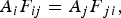
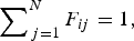
Sage Journals: Discover world-class research

Abstract

A dynamic one-dimensional mathematical model was developed for predicting the thermal state of a steelmaking ladle. The model is intended to be used in process control applications, in which fast computational times are desirable alongside model accuracy. The calculation domain was discretized using the finite difference method, and time integration was performed using both the implicit Euler and Crank–Nicolson methods, the performances of which were compared. The model was implemented in Python programming language and validated using data from our own measurements and other studies available in the literature. The results indicate that the model can reproduce the measured temperature evolution of the ladles within 5°C at best. The worst performance was observed during cooling, where the model underestimates the temperature at the innermost measurement point by up to 200°C. With computation times of around 16–23 s for one hour of simulation, the model is computationally sufficiently fast for online applications.

Introduction

The temperature of molten steel entering the casting machine is a significant quality factor in steelmaking. Insufficient temperature control not only results in a subpar product, but also in increased production disturbances. It is therefore important to have good control of the melt temperature between the melting and casting processes. The ladle’s thermal state is a significant factor affecting the melt temperature, and understanding the refractory thermal state and heat fluxes is therefore an important aspect of melt temperature control before casting. A multitude of mathematical models has been developed to better understand and monitor the ladle thermal state (see Table 1). Some of these prior models [1–7] have previously been reviewed by Fredman [8], and in the current work, the review is updated to also consider more recent models. The main characteristics of these models are discussed briefly in the following.

Table 1.

A comparison of mathematical models for the thermal state of a ladle.

Year	Study	Geometry	Model type	Key assumptions	Formulation	Use case
1973	Choné and Teyssier [1]	1D	Transient model for ladle thermal state	Uniform melt temperature		Aid ladle design work
1983	Pfeifer et al. [2]	1D	Transient model for ladle overhead thermal state	Uniform melt temperature	Finite difference equations	Design of ladle head
1984	Pfeifer et al. [3]	1D	Transient model for ladle thermal state	Uniform melt temperature	Finite difference equations	Improve casting stream temperature control
1985	Pfeifer et al. [4]	1D	Transient model for ladle thermal state	Uniform gas temperature, complete combustion		Preheating simulations, different fuels, and combustion parameters were tested
1985	Morrow and Russell [5]	1D	Transient mode for ladle thermal state	Uniform melt temperature	Finite difference equations	Ladle lining design
1986	Perkins et al. [9]	0D	Empirical model for ladle thermal state	Mean working lining temperature		Prediction of ladle thermal state
1992	Austin et al. [6]	2D	Transient model for ladle thermal state		Alternating direction implicit method with adaptive time stepping	Improve temperature control, an extensive parametric study
1993	Zoryk and Reid [7]	1D	Transient model for ladle thermal state		Finite difference equations	Online estimation of steel temperature in ladle and tundish
1998	Fredman and Saxén [10]	1D	Analytical model for ladle thermal state	Quasi-steady state outer layers, uniform melt temperature, static thermal properties, overall heat transfer coefficient approach	Analytical model, local solution by separation of variables	Rapid estimation of ladle thermal state
1999	Fredman et al. [11]	2D	Transient model for ladle thermal state	Uniform melt temperature, static thermal properties	Finite element method	Aid ladle design work
2001	Xia and Ahokainen [12]	2D	CFD-based model	Static thermal properties	CFX 4.2	Parametric study of thermal stratification
2003	Volkova and Janke [13]	1D	Transient model for the thermal state	Uniform melt temperature, overall heat transfer coefficient approach	Fourier differential equations	Study ladle lining thermal behaviour
2004	Zabadal et al. [14]	2D	Transient model for ladle furnace thermal state	Uniform melt temperature	Explicit finite difference equations	Online molten steel temperature prediction
2004	Gupta and Chandra [15]	1D	Transient model for ladle thermal state	Uniform melt temperature, static thermal properties	Finite difference equations	Online prediction of required BOF tap temperature
2006	Nath et al. [16]	1D	Transient model for ladle furnace thermal state	Uniform melt temperature		Online ladle furnace steel temperature prediction
2006	Jormalainen and Louhenkilpi [17]	2D	CFD-based model	Static material properties	CFX	A parametric study, predictive model development
2010	Samuelsson and Sohlberg [18]	1D	Parameterized transient ladle thermal state model	Uniform melt temperature	Ordinary differential equations	Estimation of molten steel temperature
2011	Glaser et al. [19]	2D	CFD-based model	Overall heat transfer coefficient for the mantle	COMSOL Multiphysics 3.5a software	Heat transfer and flow simulations for teeming
2011	Glaser et al. [20]	2D	CFD-based model	Overall heat transfer coefficient for the mantle	COMSOL Multiphysics 3.5a software	Heat transfer and flow simulations for preheating
2012	Tripathi et al. [21]	3D	CFD-based model	Static thermal properties, steel bath homogenized during online purging	Gambit software, FLUENT software	Parametric study of the steel and ladle temperature during the process cycle
2017	Deodhar et al. [22]	2D	CFD-based model	Static thermal properties, steel bath homogenized at the beginning of holding	FLUENT software	Development of a regression model
2018	Santos et al. [23]	2D	Transient model for the thermal state	Heat loss from melt top surface ignored	Abaqus software	Lining design optimization
2021	Yuan et al. [24]	2D	Transient model for the thermal state	Uniform melt temperature		Improvement of endpoint molten steel temperature prediction model
	Present study	1D	Transient model for the thermal state	Uniform melt temperature, static thermal conductivity, ladle bottom ignored	Finite difference equations implemented in Python	Fast ladle thermal state prediction

The thermal models focus on specific parts of the ladle [2] or a specific process such as preheating [4,20] or teeming [17,19]. More complex models may consider the complete process cycle and more complex geometry for the ladle. Ladle thermal models have been successfully used in parametric studies, [4,6,12,17,21] ladle design work [1,2,5,11,23], and online applications [7,14–16]. As computing power increases, two-dimensional and three-dimensional models have become more feasible model geometries. The majority of the multidimensional thermal models have been based on computational fluid dynamics (CFD) software, which offers accurate and valuable information about fluid flow and the thermal behaviour of the molten steel and ladle. However, CFD-based models are computationally too expensive for online process modelling, and instead, their results have been used to build simpler models [12,17,22] which can then be used in online applications.

The majority of the non-CFD models assume a uniform bath temperature, although there are also CFD models that assume a completely mixed melt at some point in the model cycle [21,22]. The results of Jormalainen and Louhenkilpi [17] indicate that the temperature in the ladle wall is quite uniform in the axial direction. The thermally more conductive refractory on the slag line is obviously hotter than the lower portions, but it does not seem to significantly affect the lower lining. The simplification of a uniform melt temperature may be less significant for the model results when calculating either the ladle thermal state or the average melt temperature. However, when modelling the tapping or casting temperature, the thermal stratification of the melt may significantly affect the temperature of the molten steel flow.

As computing power increases, two-dimensional models may become more feasible for online calculations. Compared to a one-dimensional model, two-dimensional ones may better account for different materials in different zones, the effects of corners, the changing view factors in different positions, and the effects of the melt height. However, with such a uniform refractory temperature along the contact surfaces, [14,17,24] their benefits may be marginal compared to a well-defined one-dimensional model.

This work aimed to develop a fast one-dimensional model for the thermal state of a steelmaking ladle. The work is based partly on the master’s thesis by Mäkelä [25], which presented the first version of the model as well as its preliminary qualitative validation. It presented and applied the main heat transfer mechanisms on the ladle wall. The calculation domain was discretized using the finite difference method. For time integration, two methods (implicit Euler and Crank–Nicolson) were implemented and compared. The model was implemented in Python programming language for fast model development. In the present study, the model is expanded to consider the top slag and the heat losses from it, and the model is validated more thoroughly using data recreated from a previous study by Fredman and Saxén [10].

Model description

Simplifications and assumptions

We made the following assumptions and simplifications:

The steel bath is completely mixed and of uniform temperature, and the refractory surface in contact with the melt is at the same temperature as the melt

Heat is conducted only in the radial direction in the ladle wall, and in the axial direction in the slag

There is no contact resistance between lining layers

Thermal conductivities of materials are constant with respect to temperature

There is no heat flux through the ladle bottom

Heat losses from the inside surfaces are caused only by radiative heat transfer

When used, the lid is closed perfectly, and there is no heat loss

During preheating, the lining surface is at the same temperature as the gas phase inside the ladle

Tapping and teeming take place instantaneously.

Nodal structure of the model

Figure 1 has a schematic example of the different nodal configurations in the model. All the reference points in the network are Δr apart from each other, and the temperature and position of the nodes are represented by T_n and r_n. The slag has a similar structure, with the exception that the relative positions of the nodes are not needed, only their distance from one another.

Figure 1.

Schematic example illustration of the nodal structure of the model.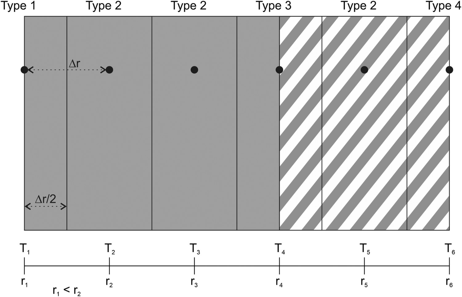

Four types of nodes were implemented for the model’s nodal network (see Figure 1):

The Type 1 node, i.e. the inner surface node in contact with the melt.

The Type 2 nodes, i.e. the bulk nodes are surrounded by a singular material and represent the bulk of the refractory or slag.

The Type 3 nodes, i.e. the boundary nodes are at the interface of two different refractory materials.

The Type 4 node, i.e. the outer surface node represents the outer surface of the ladle shell or slag.

Heat transfer mechanisms

Heat losses through the ladle wall

The ladle is modelled as a multilayer cylindrical object, for which the radial thermal conduction can be described by Equation (1),(1) where is the heat flow [W], is the height of the cylinder [m], is the thermal conductivity of the material [W K⁻¹ m⁻¹], is the temperature at the subscripted point [K], and is the radius at the subscripted point [m]. [26] It was determined (see appendix) that the dominant convection mechanism at the ladle shell at the expected shell temperatures was turbulent natural convection, which could be described using equations derived for flat vertical surfaces. Therefore convection is described by Equations (2–5),(2) (3) (4) (5) where is the convective heat transfer coefficient at the mantle [W m⁻² K⁻¹], is the surface area [m²], is the mantle surface temperature [K], is the ambient air temperature [K], Nu_wall is the dimensionless Nusselt number at the wall, Ra is the dimensionless Rayleigh number, Pr is the dimensionless Prandtl number, is gravitational acceleration [m s⁻²], is the inverse of the fluid film temperature [K⁻¹], is the vertical length [m], is the kinematic viscosity of the fluid film [m² s⁻¹], and is the thermal diffusivity of the fluid film [m² s⁻¹] [27]. Thermal radiation at the ladle surfaces is described by(6) where is the view factor, is the Stefan–Boltzmann constant [W m⁻² K⁻⁴], is the area of the radiator [m²], is the emissivity, is the temperature of the radiator [K], and is the temperature of the receiver or environment [K] [27]. The view factors for the inner ladle surfaces are calculated by first finding the view factor between the ladle bottom and the open top, which are simplified to two coaxial parallel disks. The rest of the view factors are then calculated using the reciprocity relation and the summation rule. The equations in their respective order are Equations (7), (8), and (9),(7) (8) (9) where is the view factor from surface i to j, is the radius of a subscripted surface [m], is the distance between the surfaces [m], and is the area of a subscripted surface [m²] [27].

Heat losses through the slag

The slag is modelled as a flat surface, through which the axial thermal conduction is described by Equation (10),(10) where x is the distance between the two temperatures [m] [26]. Convection from the slag surface is described by Equation (2), with Nusselt number and characteristic length being described by Equations (11) and (12),(11) (12) where is the characteristic length [m] and P is the perimeter of the flat surface [m] [27].

Material properties

Thermal conduction, radiation, and the thermal energy stored within the ladle lining greatly depend on the used materials and their temperature. Tables 2 and 3 show the thermal and emission properties of materials used in the present model. Note that for the mean specific heat of high-alumina refractory, corundum-type refractory was assumed. In the work of Glaser [20], they determined that a ladle wall with a slag layer on top, had an emissivity value of around 0.81, while the emissivity of slag was calculated to be around 0.82–0.88. We will assume the ladle wall to have a similar slag cover, and average the emissivity of the slag itself to be 0.85. The refractory temperature may also affect the ladle geometry due to thermal expansion. However, for typical refractory bricks, the expansion has been reported to be generally under 1.5% between a temperature range of 0 and 1400°C [28]. It was therefore assumed the effect of thermal expansion was negligible.

Table 2.

Thermal properties of common ladle materials.

Material	Temperature [°C]	Thermal conductivity [W K⁻¹ m⁻¹]	Mean specific heat [J K⁻¹ kg⁻¹]	Density [kg m⁻³]
High-alumina brick (Al₂O₃ = 90 wt%) [28]	100°C	3.3	860	∼3130
	500°C	2.5	1010
	1000°C	2.2	1100
	1400°C	2.3	1150
Dolomite brick [13]		4.0	1030	2860
insulating brick [13]	600°C	0.38	1500	800–900
	800°C	0.41
	1000°C	0.44
	1200°C	0.48
Carbon steel, plain carbon (Mn ≤ 1%, Si ≤ 0.1%) [27]	125°C	56.7	487	7854
	325°C	48.0	559
	525°C	39.2	685
	725°C	30.0	1169
Molten steel [19]		40	787	7000
Slag [21]		1.21	838	3807

Table 3.

Emissivity of surface materials.

Surface	Emissivity
Ladle outer shell (stainless steel, AISI 347, stably oxidized, at 326.85°C) [27]	0.87
Ladle inner wall (refractory brick, covered by slag) [20]	0.81
Slag [20]	0.85

Boundary conditions, initial conditions, and time integration

The model has been divided into three operating modes based on the different working periods of the ladle. The working periods along with the used boundary conditions are illustrated in Figure 2.

Figure 2.

Working periods of the ladle.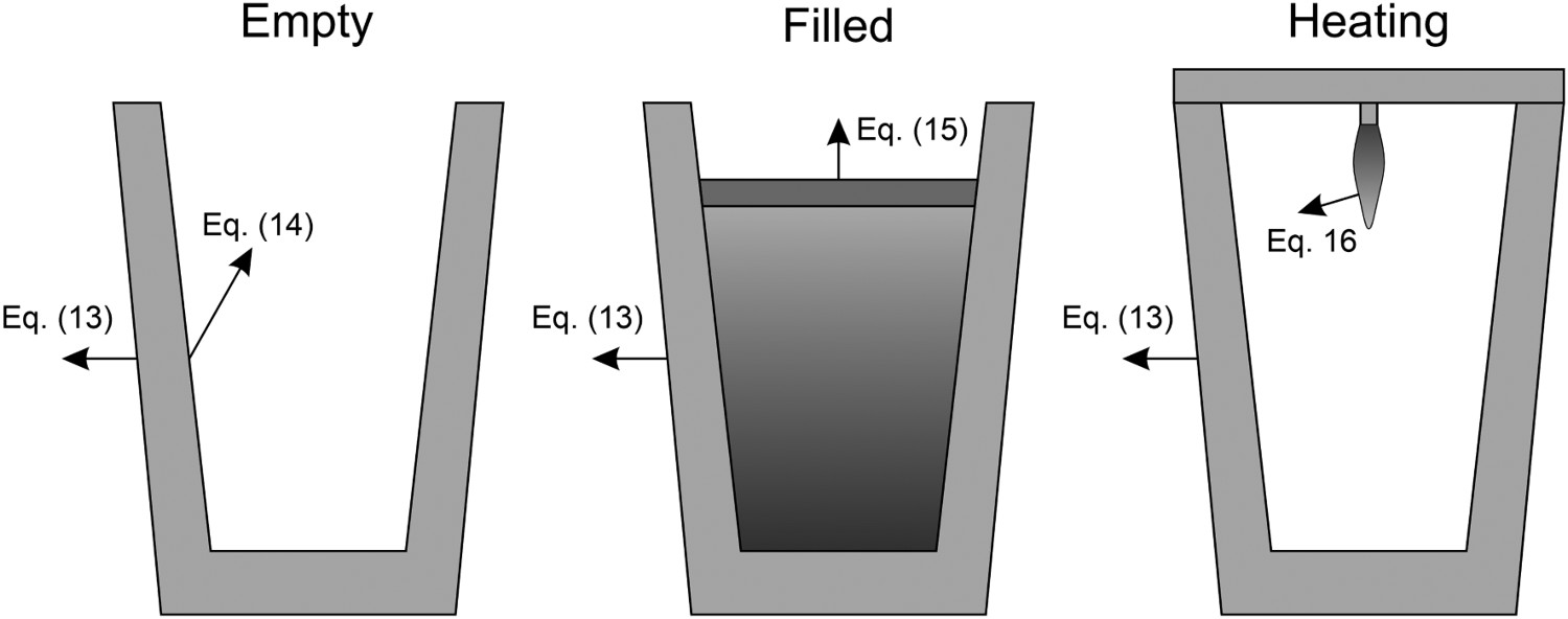

During all operating modes, the boundary condition on the ladle shell stays the same and is described by Equation (13),(13) where is the temperature of the surface [K], and is the temperature of the environment [K].

Empty period. During the empty period, the inner surface node is cooling according to grey body radiation, and transfers energy to the adjacent node through conduction. The boundary condition applied to this surface is described by Equation (14).(14)

Charged period. During the charged period, the ladle is filled with molten steel, and the inner surface node of the wall and slag are at the same temperature as the melt. The inner surface nodes transfer energy through conduction to the adjacent nodes. The boundary condition is applied to the slag top surface and is described by Equation (15).(15)

Preheating. During the preheating period, the ladle is filled with air and the inner surface node is at the same temperature as the air. The air and the inner surface node are heated according to the burner power until they reach a predetermined maximum heating temperature where it is then kept. The inner surface node transfers energy through conduction to the adjacent node. The heating is described by Equation (16),(16) where is the power of the burner [W], and is the maximum wall temperature the burner can achieve [K].

Time integration was performed using the implicit Euler and Crank–Nicolson methods. The performance of these two methods is compared in the results section. The initial conditions were chosen based on the performed validation. During the original validation, the refractory temperature profile was set to room temperature of 25°C and then heated with the burner for 36 h. Validation using data from Fredman and Saxén [10] used initial conditions, where the inner surface was at 400°C and linearly decreased to room temperature of 20°C on the outer surface. In all validations, the initial temperature of the slag was set to that of the ambient temperature.

Numerical solution

The one-dimensional temperature profile at the new time is solved using the Newton–Raphson method, by iterating Equation (17),(17) where is the current guess for the temperature profile [K], is the Jacobian matrix and is the residual vector. The iteration continues until the l₂ norm [29] of the residual between the last two solutions is less than 10⁻¹⁰. The residual vector is formed by calculating the residual of the conservation equation at each calculation node. The equations for calculating the residual in implicit Euler and Crank–Nicolson methods are written as Equations (18) and (19),(18) (19) where Res is the residual [J], is the timestep size [s], is the sum of the energy flows at the node [W], is the temperature at the node [K] at the subscripted position [m] at the superscripted time [s], is the change in the node’s energy [J]. The Jacobian matrix is obtained by partial derivation of the equations of the residual vector according to Equation (20), resulting in a tridiagonal matrix.(20)

Validation data

Measurement campaign

During the model development, a measurement campaign was conducted at the Outokumpu Stainless Oy Tornio Works, melt shop line 2. Further details regarding this production line are provided by Spiess et. al. [30]. In this campaign, the ladle mantle temperatures of 150-tonne ladles were measured with a thermal camera pointed at the casting turret.

The thermal camera had a resolution of 0.11 megapixels, a field of view of 18° by 14°, and the temperatures were given to the hundredth of a degree. The camera could not be safely calibrated at the steel plant and was therefore calibrated in laboratory conditions. To do this, a piece of generic carbon steel was fitted with a thermocouple, heated in a laboratory furnace to ∼400°C and used for calibrating the camera. The offsite calibration of the camera may have been a source of an issue, where the measurements significantly differed from the model predictions. This may have partly been due to the emissivity of the steel piece used in calibration differing from the emissivity of the steel used in the ladle shell.

Images were recorded every 4 s, whenever an object hot enough entered the field of view. The camera measured the temperatures of each pixel, allowing us to port the data into Excel, where they could then be formatted into a recreation of the thermal image. This allowed us to then process the data using commands readily available in Excel. In Figure 3, the camera positioning is shown along with a recreated thermal image, and an outlined area, from which an average temperature was taken. The area was chosen by hand from the lower portion of the ladle and covered an area of approximately 1.5–2 m². From each cast, two thermal images were chosen, one before casting and another after. The images were chosen based on quality and ladle positioning, with shaky images being ignored and importance placed on having the ladle in the same position before and after casting, allowing us to choose the same area of the ladle more consistently. From the collected data, 71 consecutive melts were chosen, which included 8 different ladles, at different stages of life.

Figure 3.

Thermal image of the ladle, and a schematic of the imaging position.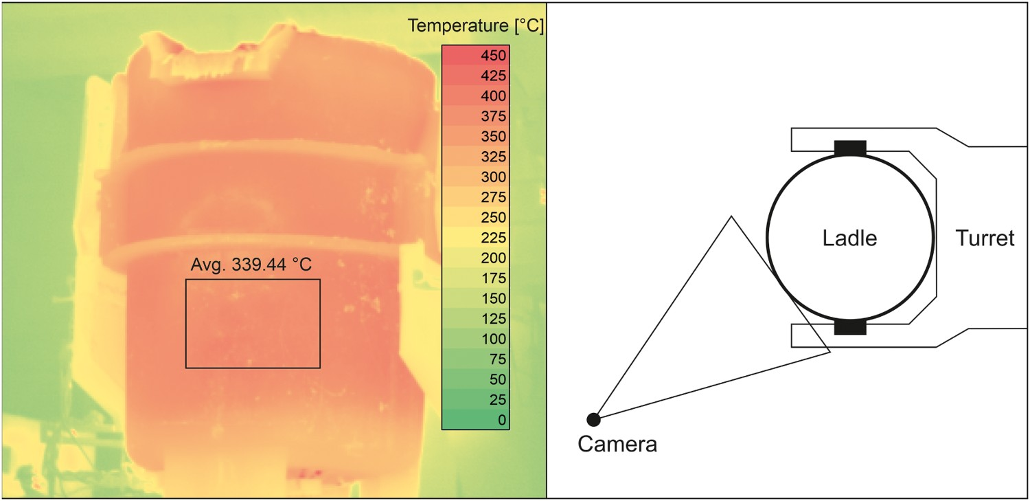

Data from the literature

In addition to our own measurements, data recreated from a previous study by Fredman and Saxén [10] was used to validate the model. Their data consisted of thermocouple measurements through the refractory and information on the length of the filled and empty periods. Their ladle had an inner radius of 1.2 m, and an outer radius of 1.44 m. The ladle had two refractory layers and a steel mantle. While the names of the refractory materials were not given, the relevant properties (thermal conductivity, specific heat, and density) were provided and are repeated in Table 4. Further details are available in Fredman and Saxén [10].

Table 4.

Material properties from Fredman and Saxén [10].

Material	Properties
Material	Thickness [m]	Thermal conductivity [W m⁻¹ K⁻¹]	Heat capacity [J kg⁻¹ K⁻¹]	Density [kg m⁻³]
Melt		36	780	7020
Air		0.024	1000	1.293
Working lining	0.155	2.5	1500	3400
Insulating lining	0.065	1.8	1200	2100
Steel shell	0.02	45	460	7800

Results and discussion

Sensitivity analysis

The effects of the Δr and Δt sizes on the model performance were studied by changing these parameters and then simulating three hours of heating, melt holding, and cooling. The temperatures of the wall inner surface and the wall outer surface nodes were logged and compared.

Tables 5 and 6 provide the tabulated temperatures of the inner surface node after three hours of simulated heating. These results are visualized more intuitively in Figure 4. The results of the implicit method significantly depend on both the Δr and Δt sizes. The Crank–Nicolson method, on the other hand, seems to depend mainly on the Δr size, with changing Δt resulting in negligible changes in results for the most part. However, the Crank–Nicolson method was prone to instability in the form of slowly dampening oscillations in the temperature profile. This was a problem mainly when using small Δr with large Δt.

Figure 4.

The temperature of the wall inner surface node after three hours of simulated heating using different time integration methods: (a) implicit Euler method, (b) Crank–Nicolson method. The black dots represent the simulated points.

Table 5.

Implicit model inner surface node temperatures after three hours of simulated heating.

Δr [mm]	Inner surface node temperature [°C]
Δr [mm]	Δt = 0.5	Δt = 1	Δt = 5	Δt = 10	Δt = 20	Δt = 40	Δt = 60
10	436.75	436.75	436.74	436.72	436.69	436.63	436.57
5	436.90	436.90	436.88	436.87	436.84	436.78	436.72
2	436.94	436.94	436.92	436.91	436.88	436.82	436.76
1	436.94	436.94	436.93	436.91	436.88	436.83	436.77

Table 6.

Crank–Nicolson model inner surface node temperatures after three hours of simulated heating.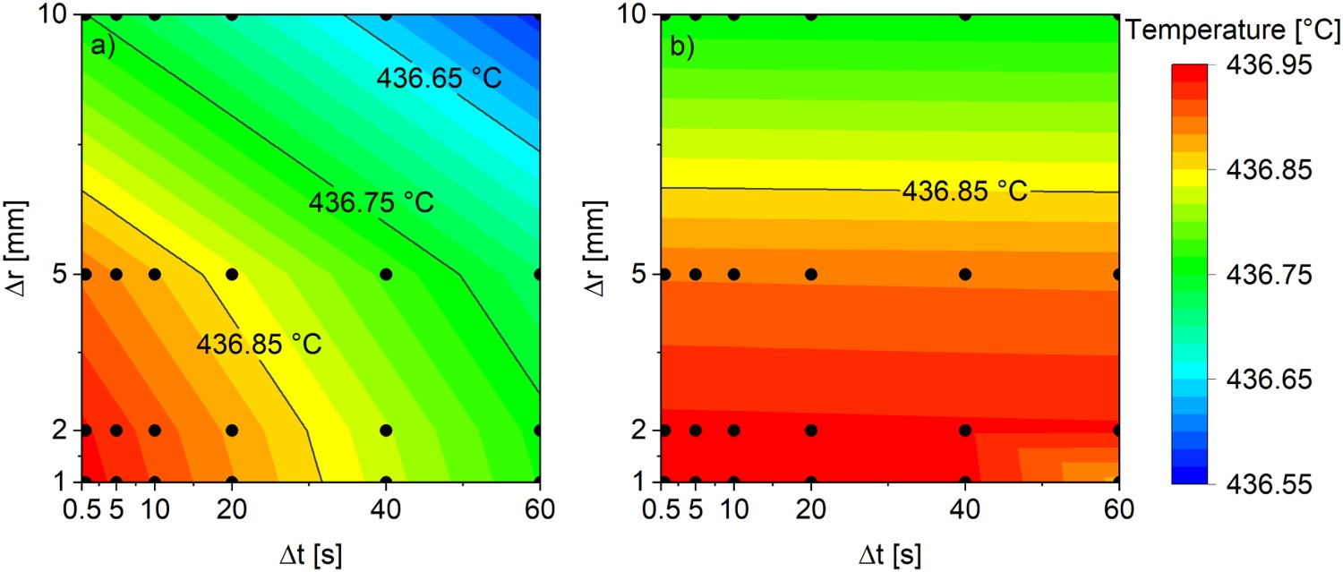

Δr [mm]	Inner surface node temperature [°C]
Δr [mm]	Δt = 0.5	Δt = 1	Δt = 5	Δt = 10	Δt = 20	Δt = 40	Δt = 60
10	436.75	436.75	436.75	436.75	436.75	436.75	436.75
5	436.90	436.90	436.90	436.90	436.90	436.90	436.90
2	436.94	436.94	436.94	436.94	436.94	436.94	436.94
1	436.94	436.94	436.94	436.94	436.94	436.94	436.88

It should be noted that the Crank–Nicolson method was around 5–20% slower than its fully implicit counterpart when using the same model parameters. However, since the result of the Crank–Nicolson method was less dependent on the used Δt, it could be faster by using larger Δt, with the risk of some instability. The instability could be resolved by applying adaptive timesteps. However, this could not be implemented in this study’s timeframe.

The implicit Euler method took around 16–23 s of real-time to simulate 1 h when using Δt = 5 s and Δr = 1 mm, on a laptop with an 11th Gen Intel Core i5-1135G7 2.40 GHz processor. This is sufficiently fast for online applications. Since the implicit method is sufficiently fast, simpler and produces almost identical results with the Crank–Nicolson method at small timestep sizes, it was deemed the more suitable option.

The data from Fredman and Saxén [10] was used to further inspect the sensitivity of the implicit model to the employed Δt and Δr, by comparing the change in the absolute error. The absolute errors from two working periods, (a) the third melt holding period and (b) the third empty period, and from three refractory positions are presented in Figure 5. The change in absolute error in all cases is quite small and should not be a cause for concern.

Figure 5.

The absolute error of the predicted temperature at three refractory positions (1.250, 1.355 and 1.440 m) at two different times: (a) third melt holding period and (b) third empty period.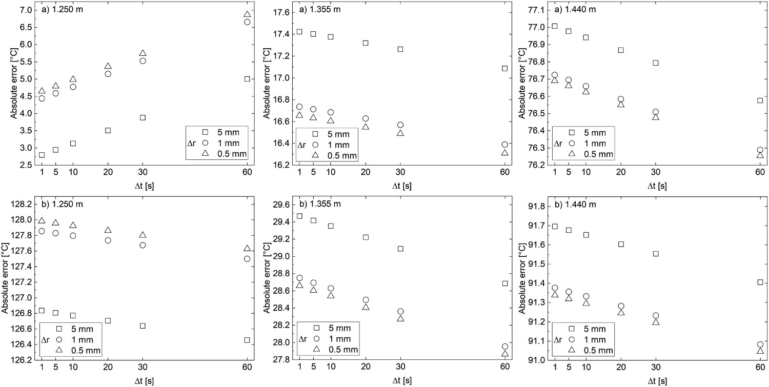

Model validation

The studied ladle has three refractory layers and a steel mantle. Starting from the hot face, the used materials were dolomite, 90% high-alumina brick, insulating brick and steel. The model was validated using the collected ladle process data to run the model and log the temperature of the steel shell at each timestep. These model results were then combined with the collected thermal imaging data, from which Figure 6 was compiled. The square marks are the measured mantle temperatures taken from the thermal images, and the black lines are the model results. The model results had to be raised by ∼100°C to obtain comparable results with the thermal images. It is suspected that this is largely caused by the inadequate calibration of the thermal camera. The temperature adjustment for each ladle is noted in Figure 6.

Figure 6.

Model validation results for the qualitative validation.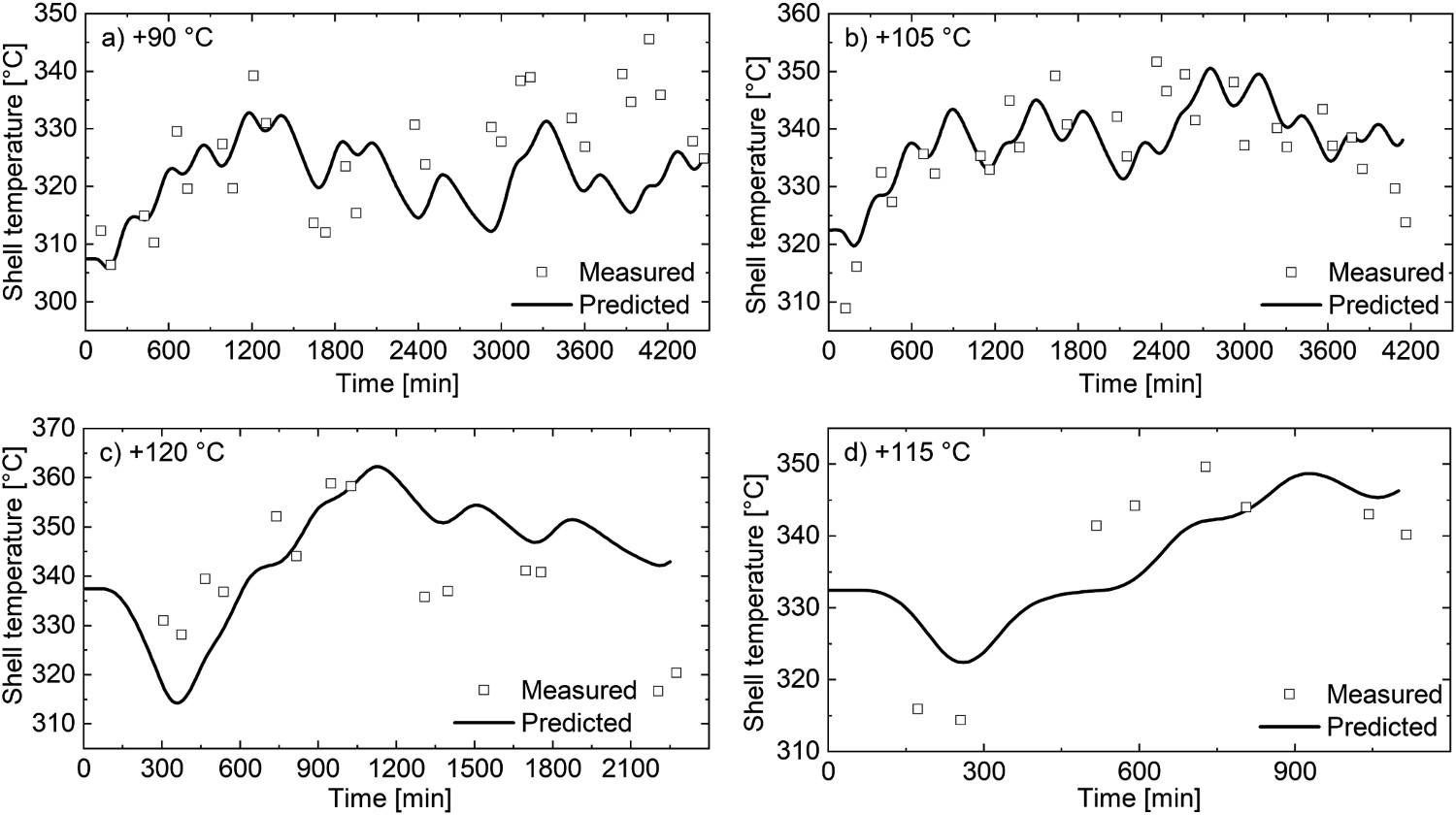

While the absolute deviations are in some cases quite large, the predicted trends are in qualitative agreement with the measured values. The inadequate validation results could be caused by improperly defined material properties, improper process data, or the overly simplistic nature of the model and its heat transfer phenomena.

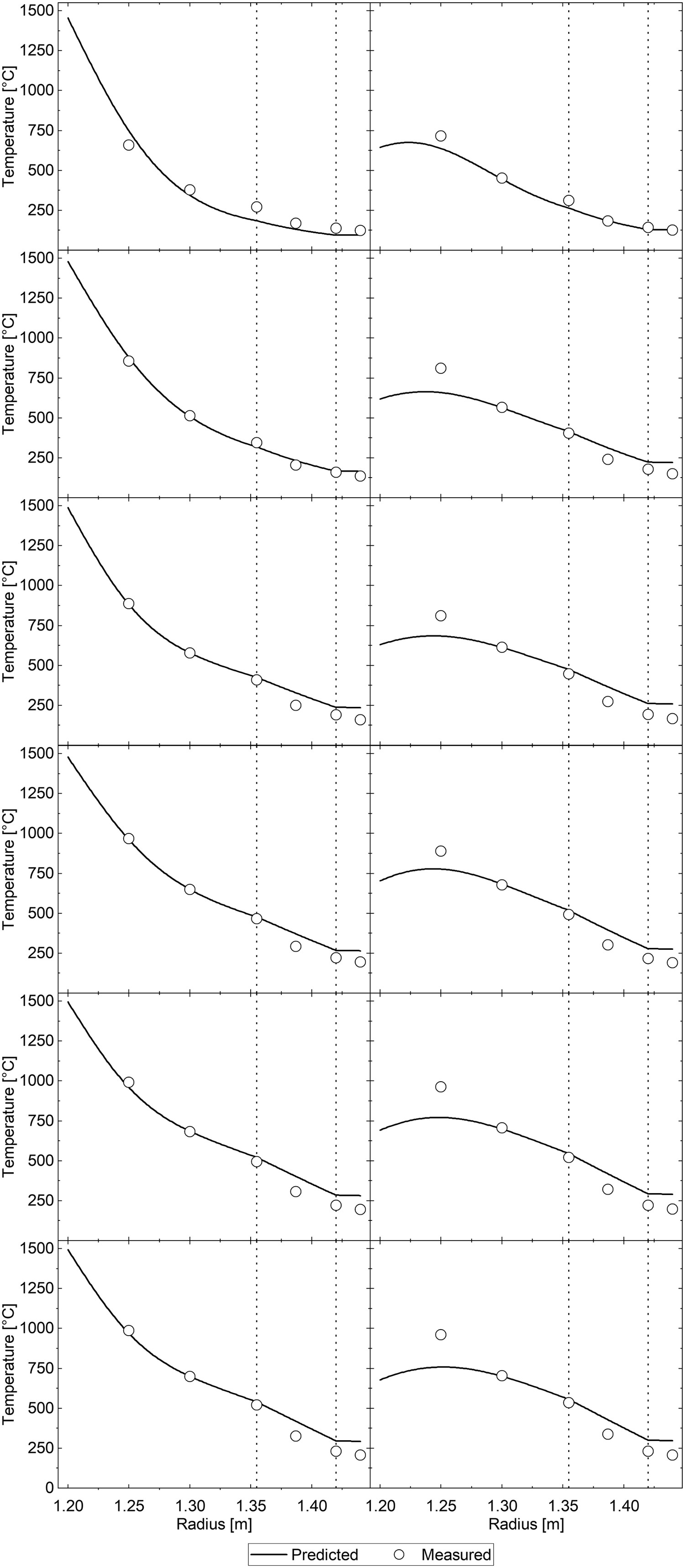
Additionally, the model was validated quantitatively using data recreated from the previous study of Fredman and Saxén. [10] It appears that the present model performs relatively well when examining the situation at the end of holding (see Figure 7). At the end of cooling, the results are noticeably worse. Figure 8 contains the predicted temperature profiles and measurements for the first six ladle cycles. It can be seen that the predicted mantle temperatures at later cycles are significantly higher than the measured values and that at the end of the cooling periods, the innermost measurement point is significantly hotter than predicted. Either our model overestimates the heat loss from the inner refractory, or some unaccounted-for process practice decreases the heat loss.

Figure 7.

Model validation results with data from Fredman and Saxén [10] at different refractory positions at two times: (a) at the end of holding and (b) at the end of cooling.

Figure 8.

Thermal profiles generated using data from Fredman and Saxén [10].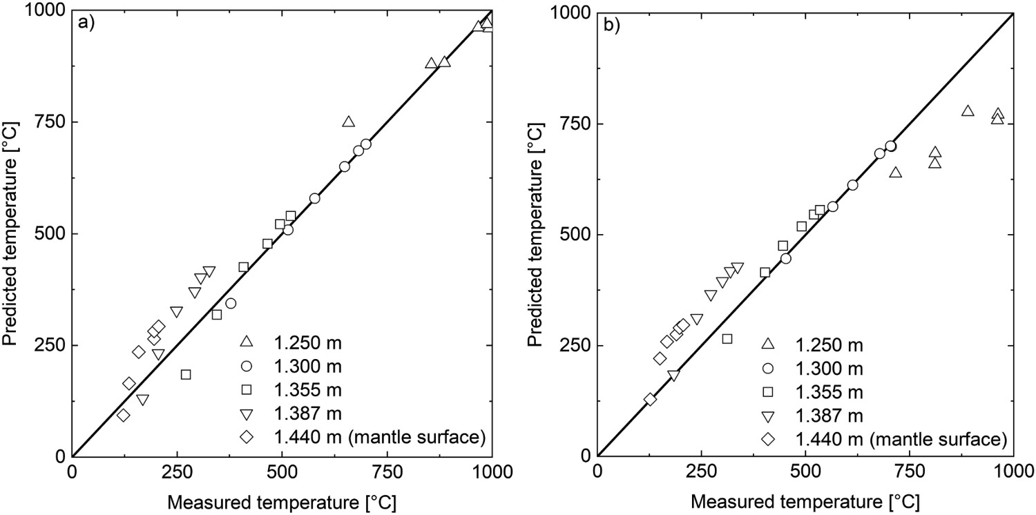

Conclusions

A dynamic one-dimensional model was developed to predict the thermal state of a ladle. The model accounts for the main heat transfer mechanism for heat losses through the ladle walls and bath surface. Two different time integration methods (implicit Euler and Crank–Nicolson) were implemented and compared. The main advantage of the Crank–Nicolson method was its insensitivity to the timestep size, which could allow the use of larger step sizes and thus shorter calculation times, provided the step sizes were not too large to cause instability. However, as the implicit Euler method was not only faster and more stable, but also produced almost identical results at smaller timesteps, it was deemed more appropriate for the intended online applications.

To validate the model, a measurement campaign was conducted in a stainless steelmaking melt shop. Based on qualitative validation using the data obtained, it was found that while the model was unable to accurately predict the short-term temperature changes at the ladle mantle, it could reproduce the main trends of temperature evolution. The next step was to conduct a quantitative validation using data available from a previous modelling study. The results suggest that the model can capture the temperature profile of the ladle wall within 5°C at best. However, the model fails to produce good predictions for the innermost refractory layer during cooling, underestimating the temperature by up to 200°C. This may have been caused by operating practices which we have not accounted for in our validation. Other than that, the next most significant error is seen on the outer shell of the ladle, where the model overestimates the temperature by around 90°C. With computation times of around 16–23 s for one hour of simulation, the employed 1D approach provides a fast basis for online temperature monitoring applications, given that the accuracy is further improved in some areas.

Footnotes

Acknowledgements

The research was carried out within the framework of the TOCANEM research programme, funded by Business Finland. The authors thank Sapotech Oy for conducting the measurement campaign at Outokumpu Stainless Oy. Furthermore, Seppo Ollila from SSAB Europe Oy and Esa Puukko from Outokumpu Stainless Oy are acknowledged for providing the technical details regarding the ladles used in this study.

Disclosure statement

No potential conflict of interest was reported by the author(s).

ORCID

Ilpo Mäkelä

Appendix

References

Choné

Teyssier

Technical report RE 137. Maizières-lès-Metz: IRSID (FR); 1973.

Pfeifer

Fett

Schäfer

et al. Der Einfluss veränderlicher Pfannenbordgeometrien auf den Wärmeverlust der Stahlschmelze. Stahl Eisen. 1983;103(25–26):1321–1326. German

Pfeifer

Fett

Schäfer

et al. Modell zur thermischen Simulation von Stahlgiesspfannen [Model for thermal simulation of steel casting ladles]. Stahl Eisen. 1984;104(24):1279–1287. German

Pfeifer

Fett

Schäfer

et al. Ein Aufheizmodell für Stahlgiesspfannen [Heating-up model for steel casting ladles]. Stahl Eisen. 1985;105(14–15):759–764. German

Morrow

Russell

RO.

Thermal modeling in melt shop applications: theory and practice. Am Ceram Soc Bull. 1985;64(7):1007–1012.

Austin

O’Rourke

, et al. Thermal modelling of steel ladles. In: 75th Steelmaking Conference proceedings; 1992 Apr 5–8; Toronto. Warrendale: Iron & Steel Society; 1992. p. 317–323.

Zoryk

Reid

PM.

On-line liquid steel temperature control. Iron Steelmaker. 1993;20(6):21–27.

Fredman

TP.

Heat transfer in steelmaking ladle refractories and steel temperature. Scand J Metall. 2000;29(6):232–258. DOI: 10.1034/j.1600-0692.2000.d01-28.x.

Perkins

Robertson

Smith

Improvements to liquid steel temperature control in the ladle and tundish. In: Scaninject IV: 4th international conference on injection metallurgy; 1986 Jun 11–13; Luleå. Luleå: MEFOS; 1986. p. 10.1–10.29.

10.

Fredman

Saxén

Model for temperature profile estimation in the refractory of a metallurgical ladle. Metall Mater Trans B. 1998;29(3):651–659. DOI: 10.1007/s11663-998-0100-4.

11.

Fredman

Torrkulla

Saxén

Two-dimensional dynamic simulation of the thermal state of ladles. Metall Mater Trans B. 1999;30(2):323–330. DOI: 10.1007/s11663-999-0061-2.

12.

Xia

Ahokainen

Transient flow and heat transfer in a steelmaking ladle during the holding period. Metall Mater Trans B. 2001;32(4):733–741. DOI: 10.1007/s11663-001-0127-2.

13.

Volkova

Janke

Modelling of temperature distribution in refractory ladle lining for steelmaking. ISIJ Int. 2003;43(8):1185–1190. DOI: 10.2355/isijinternational.43.1185.

14.

Zabadal

JRS

Vilhena

MTMB

Bogado Leite

SQ.

Heat transfer process simulation by finite differences for online control of ladle furnaces. Ironmak Steelmak. 2004;31(3):227–234. DOI: 10.1179/030192304225012150.

15.

Gupta

Chandra

Temperature prediction model for controlling casting superheat temperature. ISIJ Int. 2004;44(9):1517–1526. DOI: 10.2355/isijinternational.44.1517.

16.

Nath

Mandal

Singh

et al. Ladle furnace on-line reckoner for prediction and control of steel temperature and composition. Ironmak Steelmak. 2006;33(2):140–150. DOI: 10.1179/174328106X80082.

17.

Jormalainen

Louhenkilpi

A model for predicting the melt temperature in the ladle and in the tundish as a function of operating parameters during continuous casting. Steel Res Int. 2006;77(7):472–484. DOI: 10.1002/srin.200606417.

18.

Samuelsson

Sohlberg

ODE-Based modelling and calibration of temperatures in steelmaking ladles. IEEE Trans Control Syst Technol. 2010;18(2):474–479. DOI: 10.1109/TCST.2009.2016668.

19.

Glaser

Görnerup

Sichen

Fluid flow and heat transfer in the ladle during teeming. Steel Res Int. 2011;82(7):827–835. DOI: 10.1002/srin.201000270.

20.

Glaser

Görnerup

Sichen

Thermal modelling of the ladle preheating process. Steel Res Int. 2011;82(12):1425–1434. DOI: 10.1002/srin.201100198.

21.

Tripathi

Saha

Singh

et al. Numerical simulation of heat transfer phenomenon in steel making ladle. ISIJ Int. 2012;52(9):1591–1600. DOI: 10.2355/isijinternational.52.1591.

22.

Deodhar

Singh

Shukla

et al. Fast and accurate prediction of stratified steel temperature during holding period of ladle. Metall Mater Trans B. 2017;48(2):1217–1229. DOI: 10.1007/s11663-016-0874-8.

23.

Santos

Moreira

Campos

MGG

et al. Enhanced numerical tool to evaluate steel ladle thermal losses. Ceram Int. 2018;44(11):12831–12840. DOI: 10.1016/j.ceramint.2018.04.092.

24.

Yuan

Development of an improved CBR model for predicting steel temperature in ladle furnace refining. Int J Miner Metall Mater. 2021;28(8):1321–1331. DOI: 10.1007/s12613-020-2234-6.

25.

Mäkelä

A mathematical model for the thermal state of a steel ladle [master’s thesis]. Oulu (FI): University of Oulu; 2021.

26.

Virtaustekniikan

JA.

lämmönsiirron ja aineensiirron perusteet. Espoo: Otakustantamo; 1987.

27.

Incropera

DeWitt

Fundamentals of heat and mass transfer. New York (NY): Wiley; 1996.

28.

Technical Association of Refractories, Japan . Refractories handbook. Tokyo: Technical Association of Refractories, Japan; 1998.

29.

Horn

Johnson

CR.

Matrix analysis. Cambridge: Cambridge University Press; 1988.

30.

Spiess

Lempradi

Staudinger

et al. Technological challenges in stainless steel production at Outokumpu Stainless Tornio. Rev Metall / Cah Inf Tech. 2005;102(4):329–335. DOI: 10.1051/metal:2005103.